Mining Financial Data with Scheduled Discovery
of Exception Rules
Einoshin Suzuki
Electrical and Computer Engineering, Yokohama National University, 79-5 Tokiwadai, Hodogaya, Yokohama 240-8501, Japan
Abstract. This paper shows preliminary results, on financial data, of an algorithm for discovering pairs of an exception rule and a common sense rule under a prespecified schedule. An exception rule, which represents a regularity of exceptions to a common sense rule, often exhibits inter-estingness. Discovery of pairs of an exception rule and a common sense rule under threshold scheduling has been successful in efficient discovery of interesting rules. In this paper, we apply it to financial data, which has been provided as a benchmark data set for data mining methods. Examples of discovered knowledge as well as a simple description of the approach are both provided in this paper.
Keywords: Rule discovery, Exception Rule, Threshold Scheduling, Fi-nancial Data, Data mining.
1
Introduction
An exception rule [2–6] represents a regularity of exceptions to a common sense rule which holds true, with high probability, for many examples. An exception rule is often useful since it represents a different fact from a common sense rule, which is often a basis of people’s daily activities [5]. For instance, suppose a species of mushrooms most of which are poisonous but some of which are exceptionally edible. The exact description of the exceptions is highly beneficial since it enables exclusive possession of the edible mushrooms.
An undirected method obtains a set of pairs of an exception rule and a com-mon sense rule [3–6]. Although this approach is relatively time-consuming, it often discovers unexpected rules since it is independent of user-supplied domain knowledge. Especially, an approach proposed by Suzuki [7] obtains a set of rule pairs by appropriately updating thresholds. This update is named as “threshold scheduling”, and can potentially liberate users from worrying about specifica-tions of thresholds in discovering interesting rules. In this paper, we apply this approach to financial data, which has been provided as a benchmark data set in Discovery Challenge 2000.
2
Undirected Discovery of Exception Rules
2.1 Problem Description
Let an atom represent an event which is either a single value assignment to a discrete attribute or a single range assignment to a continuous attribute. We define a conjunction rule as a production rule of which premise is represented by a conjunction of atoms and conclusion is a single atom.
Suzuki considered a problem of finding a set of rule pairs [3–7]. Here, a rule pair r(x, x, Yµ, Zν) is defined as a pair of two conjunction rules, which are a common sense ruleYµ→xand an exception ruleYµ∧Zν→x.
r(x, x, Yµ, Zν)≡ {Yµ→x, Yµ∧Zν→x} (1) where xand x are a single atom with the same attribute but different values. Each premise of rules represents a conjunction of atoms Yµ ≡ y1∧y2∧ · · · ∧
yµ, Zν ≡z1∧z2∧ · · · ∧zν.
The method employed in this paper outputs rule pairs which satisfy
Pr(Yµ)≥θS1 (2) Pr(x|Yµ)≥MAX(θ1F,Pr( x)) (3) Pr(Yµ, Zν)≥θ2S (4) Pr(x|Yµ, Zν)≥MAX(θF2,Pr( x)) (5) Pr(x|Zν)≤MIN(θI2,Pr( x)) (6)
where Pr(x) represents the ratio of an event x in the data set, and each of θS
1, θ1F, θS2, θF2, θI2 is a threshold.
2.2 Discovery Algorithm
In an undirected discovery method for exception rules [6], a discovery task is viewed as a search problem, in which a node of a search tree represents four rule pairsr(x, x, Yµ, Zν), r(x, x, Yµ, Zν), r(x, x, Zν, Yµ), r(x, x, Zν, Yµ). Since these four rule pairs employ common atoms, this fourfold representation im-proves time efficiency by sharing calculations of probabilities of these atoms. Each node has four flags for representing rule pairs in consideration.
In the search tree, a node of depth one represents a single conclusionxorx. Likewise, a node of depth two represents a pair of conclusions (x, x). Letµ= 0 andν= 0 represent the state in which the premise of a common sense rule and the premise of an exception rule contain no atoms respectively, then we see that µ =ν = 0 holds true in a node of depth two. As the depth increases by one, an atom is added to the premise of the common sense rule or of the exception rule. A node of depth three satisfies either (µ, ν) = (0,1) or (1,0), and a node of depthl (≥4),µ+ν=l−2 (µ, ν≥1).
A depth-first search method is employed to traverse this tree, and the max-imum search depth M is given by the user. Note that M −2 is equal to the maximum value for µ+ν. Now, we introduce a theorem [7] for efficient search.
Theorem 1. LetPr(Yµ)≥Pr( Yµ), Pr( Zν)≥Pr(Zν)and a rule pair r(x, x, Yµ, Zν)satisfies at least an equation in (7) - (11), then a rule pair r(x, x, Yµ, Zν)does not satisfy all of (2) - (6).
Pr(Yµ)< θS1 (7) Pr(x, Yµ)< θS1MAX(θ F 1,Pr( x)) (8) Pr(Yµ, Zν)< θ2S (9) Pr(x, Yµ, Zν)< θS2MAX(θ2F,Pr(x)) (10) Pr(Zν)< θS2MAX(θ2F,Pr( x))/MIN(θI2,Pr( x)) (11) The proof is straightforward, and is given in [7].
If a rule pair r(x, x, Yµ, Zν) satisfies at least one of (7) - (11), the flag which corresponds to this rule pair is turned off. In expanding a search node, we define that information about flags is inherited to its children nodes. Thus, r(x, x, Yµ, Zν) is ignored in the descendant nodes without changing the output. If the four flags are all turned off in a search node, the node is not expanded.
2.3 Threshold Scheduling
Specification for values of thresholds θ1S, θS2, θ1F, θF2, θ2I is difficult in some cases.
For example, if the data set contains few exception rules, strict values result in few or no discovered patterns. We can avoid this situation by settling the values loosely, but if the data set contains many exception rules, too many patterns would be discovered at the end of long computational time. Both cases are undesirable from the viewpoint of knowledge discovery.
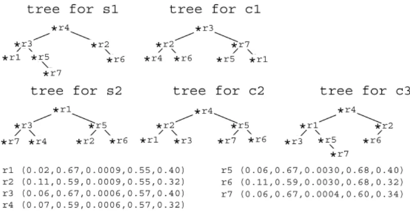
In order to cope with these problems, we have invented a novel data structure which efficiently manages discovered patterns with multiple indices. This data structure consists of several AVL trees [8] each of which has η nodes. In order to realize flexible scheduling, we assign a tree for each index. A node of a tree represents a pointer to a discovered pattern, and this enables fast transformation of the tree. We show, in figure 1, an example of this data structure which manages seven rule pairs r1, r2,· · ·, r7.
In updating values of thresholds, users either have a concrete plan or have no such plans. We show two scheduling policies for each situation. In the first policy, a user specifies threshold updating (θ1, v1),(θ2, v2),· · ·,(θξ, vξ) where θi, vi are
a threshold and its value respectively. When each AVL tree has η nodes and a new rule pair is being discovered, a value of a threshold θi is updated to vi according to current specification. Then this method deletes each stored rule pair which satisfies θi ≤vi and the nodes in the trees each of which has a pointer to the rule pair. In the second policy, a user specifies a total order to a subset of indicesPr(Yµ), Pr(Yµ, Zν),Pr( x|Yµ), Pr( x|Yµ, Zν), Pr(x|Zν). This method iteratively deletes a rule pair based on an AVL tree which is selected according to this order. Suppose each AVL tree has η nodes and a new rule pair is being discovered. If the current index isPr( x|Zν), the maximum node of the AVL tree
tree for s2 r1 * r2 * r4 * *r6 r7 * r3 * *r5 tree for c1 r1 * r3 * r4 * *r6 *r5 r2 * *r7 tree for s1
tree for c2 tree for c3
r1 * r2 * r4 * r5 * r5 (0.06,0.67,0.0030,0.68,0.40) r6 (0.11,0.59,0.0030,0.68,0.32) r7 (0.06,0.67,0.0004,0.60,0.34) r1 (0.02,0.67,0.0009,0.55,0.40) r2 (0.11,0.59,0.0009,0.55,0.32) r3 (0.06,0.67,0.0006,0.57,0.40) r4 (0.07,0.59,0.0006,0.57,0.32) r6 * r7 * r3 * r1 * *r3 r4 * r6 * r7 * *r3 r4 * r5 * *r6 r7 * r5 * r2 * *r1 *r2
Fig. 1.Illustration based on proposed data structure, where an AVL tree is employed as a balanced search-tree, and keys are s1 (Pr( Yµ)), c1 (Pr( x|Yµ)), s2 (Pr( Yµ, Zν)), c2 (Pr( x|Yµ, Zν)), c3 (Pr( x|Zν)). Numbers in a pair of parentheses represent values of these indices of the corresponding rule pair. In a tree, ∗r1,∗r2,· · ·,∗r7 represent a pointer to the rule pairs r1, r2,· · ·, r7 respectively.
for Pr(x|Zν) is deleted. Otherwise, the minimum node of current AVL tree is deleted. The same deletion procedure occurs as in the first policy, and the value of the corresponding threshold is updated. Details of the algorithms are given in [7].
3
Experimental Evaluation
3.1 Conditions
Based on the previous Discovery Challenge [1], the financial data was prepro-cessed as follows.
1) We joined “account.asc”, “disp.asc”, “card.asc”, “client.asc”, and “loan.asc”, where an example represents an account. In “disp.asc”, we only recorded the ex-istence of a second client (disponent), and ignored his client ID and account ID. The “birth number” of “client.asc” was transformed to two attributes: birth year and sex of a client.
2) We joined “district.asc” to this table which has two district IDs. These IDs concern the account and its client, and sometimes differ. In the join process, we treated these IDs individually.
3) We joined “order.asc” to this table by creating two attributes for each value “?”, “LEASING”, “POJISTN”, “SIPO”, and “UVER” of the attribute “k symbol”. These two attributes represent the total number and amount of orders. In the join process, we ignored attributes which concern the recipient.
4) We joined “trans.asc” to this table by summarizing the transactions which were executed before a loan is granted. In the join process, we considered only accounts with a loan. We created three attributes which represent the number
of transactions (TransNum), the number of days from creation of an account to the grant of a loan (TransDay), and the average balance per day (Tran-sIbal). We also created two attributes which represent the total number and amount of each type of transactions. Basically, these types were created based on the attribute “k symbol” which includes “POJISTNE”, “SLUZBY”, “UROK”, “SANKC. UROK”, “SIPO”, “DUCHOD”, and “UVER”. When the value of “k symbol” is missing, we judged the type of a transaction based on the at-tribute “operation” which includes “VYBER KARTOU”, “VKLAD”, “PRE-VOD Z UCTU”, “VYBER”, and “PRE“PRE-VOD NA UCET”.
5) Finally, we settled the task to discovering exception rules each of which concerns good loans and bad loans. We transformed the value “a”, “b”, “c”, and “d” of the attribute “loan status” to “G”, “B”, “G”, and “B” respectively. We deleted several attributes which were judged irrelevant such as IDs. We also deleted attributes which concern unemployment rates and committed crimes because several loans were granted before these statistics were available.
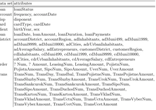
The final data set includes 69 attributes about 682 accounts. In the data set, 55 attributes are continuous, and the other attributes are nominal with 2 to 77 values. Table 1 shows these attributes. We later ignored several attributes which had a unique value for all accounts and two attributes which concern 77 district names due to time efficiency.
Table 1.Attributes of the final data set. In district, “ad” and “cd” represent account district and customer district respectively.
data set attributes loan loanStatus
account frequency, accountDate disp disponent
card cardType, cardDate client birthYear, sex
loan loanDate, loanAmount, loanDuration, loanPayments
district accountDistrict, accountRegion, adInhabitants, adMuni499, adMuni1999, adMuni9999, adMuni10000, adCities, adrUrbanInhabitants,
adAverageSalary, adEntrepreneurs, customerDistrict, customerRegion, cdInhabitants, cdMuni499, cdMuni1999, cdMuni9999, cdMuni10000, cdCities, cdrUrbanInhabitants, cdAverageSalary, cdEntrepreneurs order ? Num, ? Amount, LeasingNum, LeasingAmount, PojistnNum,
PojistnAmount, SipoNum, SipoAmount, UverNum, UverAmount
trans TransNum, TransDay, TransIbal, TransPojistneNum, TransPojistneAmount, TransSluzbyNum, TransSluzbyAmount, TransUrokNum, TransUrokAmount, TransSankcurokNum, TransSankcurokAmount, TransSipoNum,
TransSipoAmount, TransDuchodNum, TransDuchodAmount, TransKartouNum, TransKartouAmount, TransVkladNum,
TransVkladAmount, TransUctuNum, TransUctuAmount, TransVyberNum, TransVyberAmount, TransUcetNum, TransUcetAmount
3.2 Good and Bad loans
All experimental results presented in this paper are computed on several personal computers with Linux operating systems. Two indices s2(= Pr( Yµ, Zν)) and c2(=Pr(x|Yµ, Zν)) are specified in this order with the second scheduling policy presented in the previous section. In the experiments, we settled the maximum number of discovered rule pairs to η = 50 and the maximum search depth to M = 5. The attributes were discretized using the method described in [7] with the number of bins chosen as 4, 5 and 6.
In these experiments, the loan status is the only attribute allowed in the conclusions. We settled initial values of the thresholds loosely toθ1S= 0.008, θ2S= 10/682, θ1F = 0.4, θF2 = 0.4, θI2 = 0.7, and applied the proposed method. For each trial with different numbers of bins, 50 rule pairs were discovered, and the final values of the thresholds were θS2 = 0.014, 0.017, 0.024, θF2 =
0.4, 0.466, 0.444 respectively. In the applications, 4.47∗107, 1.21∗108, 3.42∗108 nodes were searched, and the number of rule pairs stored in the data structure (including those which were deleted) were 282, 316, and 276 respectively. With the use of the scheduling capability, it took only 2h40, 6h45, and 17h to obtain the results respectively. Note that these experiments were done on PCs.
Below, we show an example of rule pairs discovered in these experiments, where a “+” represents the premise of the corresponding common sense rule. We also substitutens1 (=nPr(Yµ)),ns2 (=nPr( Yµ, Zν)) andns2c2 (=nPr( x, Yµ, Zν)) fors1, s2 andc2 since they are easier to be understood, wherenis the number of examples in the data set, i.e. 682.
214≤TransDay≤393 →loanStatus = G
+ 950125≤accountDate≤970111, 13≤TransUrokNum≤35→loanStatus = B
ns1 = 225, c1 = 0.893, ns2 = 18, ns2c2 = 10, c3 = 0.107
According to this rule pair, 89.3 % of the 225 accounts whose transaction days were between 214 and 393 had good loan status. However, 10 among 18 of them (which was created between 950125 and 970111, and whose number of transactions for “urok” was between 13 and 35 in addition to the above condition) had bad loan status. This exception rule is unexpected and interesting since only 10.7 % of the account which was created between 950125 and 970111, and whose number of transactions for “urok” was between 13 and 35 had bad loan status.
Below are other examples of discovered rule pairs.
100 ≤ customer district Entrepreneurs ≤ 167, 16 ≤ TransUrokNum ≤ 57 → loanStatus=G
+ 6≤TransSipoNum≤9→loanStatus = B
1901≤UverAmount≤9910, 1≤TransSipoNum≤9→loanStatus = G + 16 ≤TransUrokNum≤35→loanStatus = B
ns1 = 189, c1 = 0.888, ns2 = 20, ns2c2 = 9, c3 = 0.104 16≤TransUrokNum≤35→loanStatus = G
+ 1901 ≤loanPayments≤9910, 1≤TransSipoNum≤9→loanStatus = B ns1 = 230, c1 = 0.895, ns2 = 20, ns2c2 = 9, c3 = 0.111 5.82≤TransUrokAmount≤15.93 →loanStatus = G + 529.41 ≤TransIbal ≤ 41725.33, 364.31 ≤TransUctuAmount ≤ 1965.37 → loanStatus = B ns1 = 274, c1 = 0.901, ns2 = 12, ns2c2 = 6, c3 = 0.108 1948≤birthYear≤1958→loanStatus = G
+ 42821≤account district Inhabitants≤88884, 1≤? Num≤2→loanStatus = B ns1 = 177, c1 = 0.903, ns2 = 11, ns2c2 = 5, c3 = 0.096 529.41 ≤ TransIbal ≤ 38594.03, 364.31 ≤ TransUctuAmount ≤ 1965.37 → loanStatus=G +5.33≤TransUrokAmount≤15.93→loanStatus = B ns1 = 85, c1 = 0.894, ns2 = 12, ns2c2 = 5, c3 = 0.099 2≤PojistnAmount≤9115→loanStatus = G
+1948≤birthYear≤ 1958, 42821≤cdInhabitants ≤122603→ loanStatus = B
ns1 = 114, c1 = 0.912, ns2 = 12, ns2c2 = 5, c3 = 0.104 accountRegion = centralBohemia→loanStatus = G
+ 106 ≤customer district Entrepreneurs ≤ 114, 4.15≤ TransUrokAmount≤ 6.83→loanStatus = B
ns1 = 90, c1 = 0.888, ns2 = 12, ns2c2 = 5, c3 = 0.102
529.41≤TransIbal≤38594.03, 3≤TransUctuNum≤24→loanStatus=G + loanDuration = 12→loanStatus = B
ns1 = 85, c1 = 0.894, ns2 = 12, ns2c2 = 5, c3 = 0.083
4
Conclusions
In this paper, we applied, to the financial data, simultaneous discovery of an exception rule and a common sense rule with a scheduling capability [7]. The method updates values of multiple thresholds appropriately according to the discovery process, and discovers appropriate number of rule pairs in reasonable time. Several examples of rule pairs are shown as preliminary results.
Acknowledgement
This work was partially supported by the grant-in-aid for scientific research on priority area “Discovery Science” from the Japanese Ministry of Education, Science, Sports and Culture.
References
1. P. Berka: Workshop Notes on Discovery Challenge, Univ. of Economics, Prague, Czech Republic (1999).
2. B. Padmanabhan and A. Tuzhilin: “A Belief-Driven Method for Discovering Unex-pected Patterns”,Proc. Fourth Int’l Conf. Knowledge Discovery and Data Mining (KDD), AAAI Press, Menlo Park, Calif., pp. 94–100 (1998).
3. E. Suzuki and M. Shimura : Exceptional Knowledge Discovery in Databases Based on Information Theory, Proc. Second Int’l Conf. Knowledge Discovery and Data Mining (KDD), AAAI Press, Menlo Park, Calif., pp. 275–278 (1996).
4. E. Suzuki: “Discovering Unexpected Exceptions: A Stochastic Approach”, Proc. Fourth Int’l Workshop Rough Sets, Fuzzy Sets, and Machine Discovery (RSFD), Japanese Research Group on Rough Sets, Tokyo, pp. 225–232 (1996).
5. E. Suzuki: “Autonomous Discovery of Reliable Exception Rules”,Proc. Third Int’l Conf. Knowledge Discovery and Data Mining (KDD), AAAI Press, Menlo Park, Calif., pp. 259–262 (1997).
6. E. Suzuki and Y. Kodratoff: “Discovery of Surprising Exception Rules based on Intensity of Implication”, Principles of Data Mining and Knowledge Discovery (PKDD), LNAI 1510, Springer-Verlag, Berlin, pp. 10–18 (1998).
7. E. Suzuki: “Scheduled Discovery of Exception Rules”, Discovery Science (DS), LNAI 1721, Springer-Verlag, Berlin, pp. 184–195 (1999).
8. N. Wirth: Algorithms + Data Structures = Programs, Prentice-Hall, Englewood Cliffs, N.J. (1976).