Cluster-Based Chained Transfer Learning for Energy Forecasting With Big Data

(1)

Western University Western University

Scholarship@Western

Electronic Thesis and Dissertation Repository

12-12-2019 12:30 PM

Cluster-Based Chained Transfer Learning for Energy Forecasting

With Big Data

Yifang Tian

The University of Western Ontario Supervisor

Grolinger, Katarina

The University of Western Ontario

Graduate Program in Electrical and Computer Engineering

A thesis submitted in partial fulfillment of the requirements for the degree in Master of Engineering Science

Follow this and additional works at: https://ir.lib.uwo.ca/etd

Part of the Industrial Engineering Commons, Other Computer Engineering Commons, and the Other Electrical and Computer Engineering Commons

Recommended Citation Recommended Citation

Tian, Yifang, "Cluster-Based Chained Transfer Learning for Energy Forecasting With Big Data" (2019). Electronic Thesis and Dissertation Repository. 6778.

https://ir.lib.uwo.ca/etd/6778

This Dissertation/Thesis is brought to you for free and open access by Scholarship@Western. It has been accepted for inclusion in Electronic Thesis and Dissertation Repository by an authorized administrator of

(2)

Abstract

Smart meter popularity has resulted in the ability to collect big energy data and has created opportunities for large-scale energy forecasting. Machine Learning (ML) techniques com-monly used for forecasting, such as neural networks, involve computationally intensive train-ing typically with data from a strain-ingle buildtrain-ing/group to predict future consumption for that same building/group. With hundreds of thousands of smart meters, it becomes impractical or even infeasible to individually train a model for each meter. Consequently, this paper proposes Cluster-Based Chained Transfer Learning (CBCTL), an approach for building neural network-based models for many meters by taking advantage of already trained models through transfer learning. CBCTL first clusters the meters based on their load profiles. Next, Similarity-Based Chained Transfer Learning (SBCTL) is applied within each cluster; the first model within each cluster is trained in a traditional way and all other models transfer knowledge from existing models in a chain-like manner according to similarities between energy consumption profiles. A Recurrent Neural Network (RNN) was used as the base forecasting model, two initialization techniques were considered, and different similarity measures were explored. The experiments show that CBCTL and SBCTL achieve accuracy comparable to traditional ML training while taking only a fraction of time.

Keywords: transfer learning, deep learning, energy forecasting, recurrent neural network, gated recurrent units, smart meters, Big Data.

(3)

Summary for Lay Audience

Smart meter popularity has resulted in the ability to collect big energy data and has cre-ated opportunities for large-scale energy forecasting. The algorithms that commonly used for energy forecasting, involve computationally intensive training typically with data from a sin-gle building/group to predict future consumption for that same building/group. With hundreds of thousands of smart meters, it becomes impractical or even infeasible to individually train a model for each meter. Consequently, this paper proposes Cluster-Based Chained Transfer Learning (CBCTL), an approach for building forecasting models for many meters by taking advantage of already trained models. CBCTL first groups the meters based on their usage patterns. Next, Similarity-based Chained Transfer Learning (SBCTL) is applied within each grouped meter; the first model within each cluster is trained in a traditional way and all other models transfer knowledge from existing models in a chain-like manner according to similar-ities between usage patterns. A Recurrent Neural Network (RNN) was used as the base fore-casting model, two initialization techniques were considered, and different similarity measures were explored. The experiments show that CBCTL and SBCTL achieve accuracy comparable to traditional ML training while taking only a fraction of time.

(4)

Acknowledgements

First of all, I would like to express my deep gratitude to my supervisor Katarina Grolinger. The faith that she has put in me is the primary reason for all these valuable outcomes. She has recognized me from her class two years ago and continually offered her support with great patience. Throughout this bite of research life, I can feel my improvement in deep learning knowledge, paper writing skills, critical thinking, and enthusiasm of research. During our meeting, she would always cheer me up when I seemed discouraged or stressful. In conclusion, I felt so lucky that I have met the kindest supervisor ever.

I would also like to thank my families for their encouragement and advice. My mom, Xuelan, takes care of everything back home so that I won’t need to worry about anything else except for my research. My dad, Xiaolong, chasing your step is my main motivation, I just want to make you proud. Jingyi, thank you for always watching over my back. I really enjoy all the time that we have spent together which is my happiest moment. I believe you are the right one.

Also to my friends, Junfei, Ljubisa, Ananda, Navid, Santiago, and Norm, thank you for your support on my research along the way. Nobody knows how many coffees we have shared and how many scratching we have done together on the whiteboard. The world of machine learning unfolds in front of me with you guys by my side.

At last, thank Utilismart, an industrial partner, for allowing me to work with a great team. This is such a valuable experience for me.

(5)

5.3.1 Data set . . . 44 5.3.2 Experiment . . . 45 5.3.3 Result . . . 45 5.4 Experiment Three . . . 48 5.4.1 Data set . . . 49 5.4.2 Experiment . . . 49 5.4.3 Result . . . 49 5.5 Discussion . . . 51 6 CBCTL Evaluation 53 6.1 Evaluation Process . . . 53 6.2 Experiment . . . 55 6.3 Results . . . 58 6.3.1 Direct Clustering . . . 58 6.3.2 Indirect Clustering . . . 61 6.4 Discussion . . . 62

7 Conclusion and Future Work 65 7.1 Conclusion . . . 65

7.2 Future Work . . . 67

Bibliography 69

Curriculum Vitae 74

(8)

List of Figures

2.1 An example of feed-forward neural network. . . 7

2.2 An RNN neuron unfolded in time. . . 8

2.3 GRU cell structure. . . 9

2.4 Traditional machine learning and transfer learning. . . 11

4.1 The CBCTL algorithm. . . 23

4.2 Sliding window technique. . . 26

4.3 Direct Clustering seasonal profile. . . 28

4.4 Indirect Clustering seasonal profile. . . 29

4.5 Chained transfer learning. . . 31

4.6 Similarity-Based Chained Transfer Learning (SBCTL). . . 31

4.7 Sequence-to-Sequence recurrent neural network. . . 34

5.1 Daily load profile - meter 4. . . 40

5.2 Daily load profile - meter 5. . . 40

5.3 SBCTL Predicted vs Actual: Zoom last 7 days. . . 42

5.4 Experiment 1: Test set MAE for SBCTL and traditional ML. . . 43

5.5 Experiment 1: Test set MAPE for the two SBCTL paths. . . 44

5.6 Experiment 2: Mean MAPE and MAE for different distance metrics. . . 46

5.7 Experiment 2: Test set MAPE for SBCTL and traditional ML. . . 47

5.8 Experiment 2: Test set MAPE at first and fifth epoch. . . 48 5.9 Experiment 3: MAPE and MAE for different initializations and distance metrics. 50

(9)

6.1 Direct Clustering evaluation. . . 59

6.2 Direct Clustering: Cluster 6 patterns. . . 60

6.3 Indirect Clustering evaluation. . . 63

6.4 Indirect Clustering: Cluster 6 patterns. . . 64

(10)

List of Tables

5.1 Example data from forecasting data set . . . 40

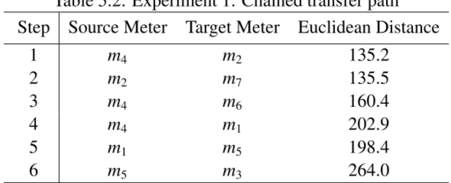
5.2 Experiment 1: Chained transfer path . . . 41

5.3 Experiment 1: Average training time . . . 43

5.4 Experiment 2: Chained transfer path . . . 45

5.6 Experiment 3: MAPE and MAE for initializations A and B, for each distance metrics . . . 50

6.1 CBCTL chained transfer path . . . 58

6.2 Direct Clustering: Accuracy comparison between approaches . . . 61

6.3 Indirect Clustering: Accuracy comparison between approaches . . . 62

6.4 Elapsed time comparison between approaches . . . 64

(11)

List of Abbreviations, Symbols, and Nomenclature

ML Activities of Daily Life

SBCTL Similarity-based Chained Transfer Learning CBCTL Cluster-based Chained Transfer Learning

NN Neural Network

SVM Support Vector Machine

RNN Recurrent Neural Network

FFNN Feed-forward Neural Network

BPTT Back-propagation Through Time

LSTM Long-short Term Memory

GRU Gated Recurrent Unit

S2S Sequence to Sequence

DI Dunn Index

DBI Davie-Brown Index

GP Genetic Programming

SVR Support Vector Regression

ANN Artificial Neural Network

DNN Deep Neural Network

(12)

SMLE Stacking Multi-Learning Ensemble

ARIMA Autoregressive Integrated Moving Average

GA Genetic Algorithm

CNN Convolutional Neural Network

MRI Magnetic Resonance Images

NLP Natural Language Processing

DBSCAN Density-Based Spatial Clustering of Applications with Noise

DTW Dynamic Time Warping

MAPE Mean Absolute Percentage Error

MAE Mean Absolute Error

CUDA Compute Unified Device Architecture

RMSE Root Means Square Error

CV Coefficient of Variance

(13)

Chapter 1

Introduction

1.1

Motivation

Smart meters are being installed in industrial, commercial, and residential buildings at increas-ing rates: presently there are over 70 million smart meters in the USA and over 96 million in China [1]. A number of smart meters together with their possibly frequent reading intervals results in a massive quantity of electricity consumption data. These Big Data have created new opportunities for analyzing energy use, designing demand-response programs, identifying savings opportunities, and measuring energy efficiency, but they also caused challenges related to processing such large data.

Energy forecasting has been attracting significant research interest because of the increased importance of preserving the environment, availability of smart meter data, and forecasting importance for both, retailers [2] and consumers [3]. Sensor-based energy forecasting relies on historical data from smart meters or other sensors, often in conjunction with meteorological information, to infer future energy consumption. Examples of Machine Learning (ML) tech-niques used for this task include Neural Networks (NN) [4], Support Vector Machine (SVM) [4], and their variants [5]. These ML techniques achieve good accuracy [6]; however, they are typically computationally complex and, with a high number of readings, it may be

(14)

2 Chapter1. Introduction

consuming to train a prediction model even for a single building/meter [7].

Recently, Recurrent Neural Networks (RNN) have outperformed other energy forecast-ing models [8]. An RNN is a type of NN where connections span adjacent time steps and form a directed graph along a temporal sequence. This makes them suitable for capturing time-dependencies and for dealing with time-series data such as smart meter data. Because of spanning adjacent time steps, the total number of connections among neurons in an RNN is larger than in a traditional feed-forward neural network. Consequently, the number of weights to learning during training is increased, and so is the training time.

Many machine learning techniques, including RNNs, require training a forecasting model with historical data from a single building or a group of buildings to predict future consumption for that same building or the group of buildings. As training even a single forecasting model can be computationally expensive and time-consuming [7], repeating the same process for hundreds of thousands of meters becomes impractical or even infeasible.

Transfer learninghas been identified as one of the open research areas in smart meter data analytics [1]; it is motivated by the fact that people can intelligently apply knowledge learned in the past to solve new problems in a new context in a faster and/or better way [9]. In traditional ML, models are built for a specific domain (e.g. specific smart meter) and task (e.g. energy prediction), and then used for the same domain and task (e.g. predict future consumption for the same meter). On the other hand, transfer learning aims to take advantage of knowledge gained on one domain/task and apply it to a different domain/task. Consequently, transfer learning has the potential to enable training machine learning models for many meters/buildings without the computational cost involved with training each model separately.

The research in energy forecasting domain has been mainly concerned with a single meter, building, or aggregated load [7, 10, 11] with the ML model trained solely on data from the same entity. Transfer learning has the potential to enable training energy forecasting models on a large scale by exploiting similarities between energy consumption profiles. Consequently, this thesis explores accelerating the training process of a large number of energy forecasting

(15)

1.2. Contributions 3

models by taking advantage of transfer learning.

1.2

Contributions

The main contributions of this thesis can be summarized as follows:

• Similarity-Based Chained Transfer Learning (SBCTL) algorithm is a novel solution for building neural network-based forecasting models for a large number of smart meters. The model for the first meter is trained in a traditional manner using a RNN; hyperpa-rameters are optimized and weights learned using data from that meter. Next, the model is built for the meter with the energy consumption pattern the most similar to the pattern of the first meter, but the training process starts with the pre-trained model from the first meter. The process continues in a chain-like manner according to similarities in energy consumption patterns. Hence, the specific contribution is in reducing the training time of building forecasting models for a large number of meters without significant loss of accuracy.

• Cluster-Based Chained Transfer Learning (CBCTL) algorithm has the same objective as SBCTL: building neural network-based forecasting models for a large number of smart meters. The main difference between CBCTL and SBCTL is that CBCTL uses clustering techniques to improve the performance of the chained transfer learning. CBCTL first applies K-means clustering to group smart meters according to similarities of their load profiles. Then, within each cluster, the forecasting models are built following the SBCTL algorithm. The combination of load profile clustering and transfer learning for energy forecasting is the specific contribution.

• Evaluation of SBCTL on three different data sets, one proprietary data set and two open-source data set. The largest data set contains 456 smart meters to test the abilities of SBCTL on a large data set.

(16)

4 Chapter1. Introduction

• Evaluation of SBCTL with two different initializations and four different distance metrics. To determine better SBCTL initialization method and its relationship with the similar-ity score, the chained transfer process is initialized from the center and from the most similar pair of meters. The forecasting accuracy is compared for the two idealizations. To explore the effect of the distance metrics on the chained transfer learning path, the four metrics are evaluated: Euclidean, Cosign, Manhattan and Dynamic Time Warping (DTW) distance. These metrics result is different transfer paths and different forecasting accuracies.

• Evaluation of CBCTL with two different clustering approaches and with different number of clusters. Based on different feature generation techniques, direct clustering and indirect clustering are explored and discussed. Also, K-means clustering with varying number of clusters is applied and evaluated. The results were examined taking the forecasting accuracy as the evaluation criteria.

• Comparison between CBCTL, SBCTL, and traditional ML training: The three approaches are evaluated in terms of forecasting accuracy and computation time. This evaluation also shows how SBCTL behaves when used standalone and how when used as part of CBCTL.

In all experiments with different data sets, CBCTL and SBCTL achieved accuracy com-parable to traditional ML training while taking only a fraction of time. CBCTL outperformed SBCTL in terms of overall forecasting accuracy.

1.3

Thesis Outline

The rest of the thesis is organized as follows: Chapter 2 describes the background, which includes feed-forward neural networks in Section 2.1, recurrent neural networks in Section 2.2, transfer learning in Section 2.3, and clustering in Section 2.4.

(17)

1.3. ThesisOutline 5

Chapter 3 discusses the related work. First, energy forecasting works are discussed in Section 3.1. followed by a review of transfer learning in the energy domain as well as other domains. Finally, Section 3.3 introduces the research regarding load profile clustering.

Chapter 4 presents the core of the thesis, Cluster-Based Chained Transfer Learning(CBCTL) algorithm. Section 4.1 provides the overview of CBCTL and Section 4.2 explains the data preparation process. Section 4.3 presents the load profile clustering, while Section 4.4 de-scribes the Similarity-Based Chained Transfer Learning (SBCTL).

Chapter 5 explains the experiments conducted with SBCTL and the corresponding results. Section 5.1 discusses the evaluation process while sections 5.2 - 5.4 present three experiments on different data sets. The findings are summarized and discussed in Section 5.5.

Chapter 6 describes the experiments conducted with CBCTL and presents the comparison with other algorithms. The evaluation process is described in Section 6.1 and the experiment is depict in Section 6.2. Section 6.3 presents the results and analyzes the findings. Finally, Section 6.3 discusses the results and summarizes the findings.

(18)

Chapter 2

Background

This section introduces the feed-forward neural networks, recurrent neural networks, the trans-fer learning concepts, and the clustering. These machine learning techniques are components that have been used in designing CBCTL.

2.1

Feed-Forward Neural Network

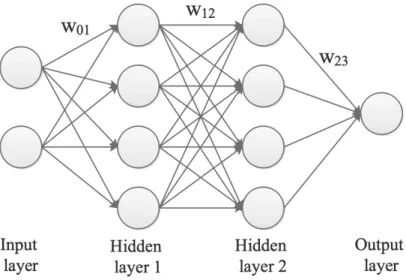
Neural networks (NN) are machine learning models inspired by the biological neurons in the human brain. They have achieved success in many tasks, such as energy forecasting [5], human activity recognition [12], and stock price forecasting [13]. As shown in Fig. 2.1, the commonly used feed-forward neural network (FFNN) consists of interconnected neurons organized in an input layer, hidden layers, and an output layer [11]. Neurons in each hidden layer are fully connected with neurons in the preceding and the subsequent layer; however, there are no connections among neurons in the same layer. The information flows from the input layer, through the hidden layer(s), to the output layer.

The neural network training process starts with initializing weightswbetween neurons to random values [14]; this initial state if referred to asthe seed. The training samples are passed forward through the network, the objective function is calculated, and back-propagation is applied to minimize the objective function by updating the weights w[14]. Anepochsrefers

(19)

2.2. RecurrentNeuralNetwork 7

Figure 2.1: An example of feed-forward neural network.

to one forward pass and one backward pass of all training data; training typically requires a number of epochs for weights to converge. When the weights are updated using gradient descent, there is a possibility of the network getting stuck in a local minimum. To avoid this, training is often repeated by starting from different initial random states or seeds.

2.2

Recurrent Neural Network

Recurrent neural networks (RNNs) are artificial neural networks where connections between nodes form a directed graph along a temporal sequence [10]. RNN cells contain internal states capable of remembering information in sequential time steps, which makes them well-suited for time series forecasting tasks such as energy prediction.

Fig. 2.2 shows an RNN neuron and its representation unfolded in time. Here, x, o and s represent the inputs, outputs and states, and indextrefers to a time step. In traditional RNNs, the weights ware updated using back-propagation through time (BPTT) algorithm; however, this method suffers from the vanishing gradient problem [15]. To overcome this issue, Long Short-Term Memory (LSTM) cell was introduced. The LSTM cell contains three gates (input i, forget f and output o), an update step g, a cell memory state c and a hidden state h. The

(20)

8 Chapter2. Background

computations in a single LSTM cell at timet, for input x, is shown as [16]:

it =σ(Wxix[t]+bxi+Whih[t−1]+bhi) (2.1a) ft =σ(Wx fx[t]+bx f +Wh fh[t−1]+bh f) (2.1b) gt =tanh(Wxgx[t]+bxg+Whgh[t−1]+bhg) (2.1c) ot =(Wxox[t]+bxo+Whoh[t−1]+bho) (2.1d) c[t] = ftc[t−1]+itgt (2.1e) h[t] =ottanh(c[t−1]) (2.1f)

Here, tanh represents the hyperbolic tanh activation function, σis the sigmoid activation function and element-wise multiplication is denoted as. TheWx’s are the weight metrics for

input-hidden, andWh’s are the hidden-hidden weight metrics learned during training. Similarly,

the biases learned during training are represented withbx’s andbh’s.

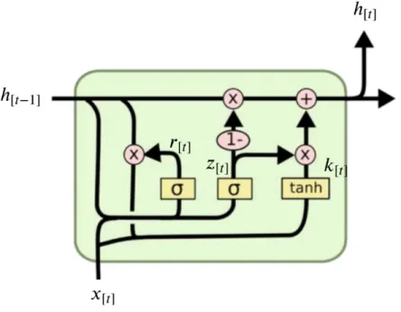
To simplify LSTM while still maintaining its core functionality, the Gated Recurrent Unit (GRU) cell was introduced [17]. The GRU cell helps with the gradient vanishing problem comparing to vanilla RNN cell and the GRU call has fewer weights than LSTM cell making it faster to train. The GRU cell architecture is shown in Fig. 2.3 [17]. GRU cells merge LSTM input and forget gates into an update gatezand combine the cell memory state and hidden state into a single hidden stateh. Also, the reset gater is introduced to reduce the previous hidden

(21)

2.2. RecurrentNeuralNetwork 9

state’s impact on the new hidden statek. A single GRU cell computations are given as [17]:

r[t]= σ(Wxrx[t]+bxr+Whrh[t−1]+bhr) (2.2) z[t]= σ(Wxzx[t]+bxz+Whzh[t−1]+bhz) (2.3) k[t]= tanh(Wxkx[t]+bxk+rt(Whkh[t−1]+bhk)) (2.4) h[t]= (1−z[t])k[t]+z[t]h[t−1] (2.5)

where σ is the sigmoid activation function, tanh is the hyperbolic tanh activation function, andrepresents element-wise multiplication. The input-hidden weight matrices areWx’s and

hidden-hidden weight matrices are Wh’s. Similarly, the bx’s and bh’s are the corresponding

biases.

Sequence to Sequence (S2S) RNNs have been extensively used for language translation and recently have demonstrated success in energy forecasting [8]. They consist of two RNNs, an encoder and decoder RNN, which improves consecutive sequence prediction.

SBCTL proposed here is designed for use with any neural network-based algorithm. We chose to evaluate it with GRU S2S-RNN proposed by Sehovacet al.[8] because this

(22)

ture outperformed other RNNs as well as feed-forward neural networks in energy forecasting tasks [8].

2.3

Transfer Learning

Transfer learning is a machine learning approach where knowledge gained while performing a task in one domain is used to improve learning in a different domain or applied for a different task [9]. It is defined as follows [9]:

Transfer Learning: Given a source domainDS and learning taskTS, a target domainDT and

learning taskTT, transfer learning aims to help improve the learning of the target predictive

functionrT(·) in DT using the knowledge inDS andTS, whereDS , DT, orTS ,TT. [9]

Here, a domain is a pairD={F,P(X)}, whereF ={f1, ..., fk}is a feature space consisting of kfeatures. Xis a set of learning samplesX = {x1, ...,xm}, andP(X) is the marginal probability

distribution ofX. Domains are considered different if either marginal probability distributions or feature spaces are different. In this research, smart meter readings with associated date/time attributes make up the learning samplesX.

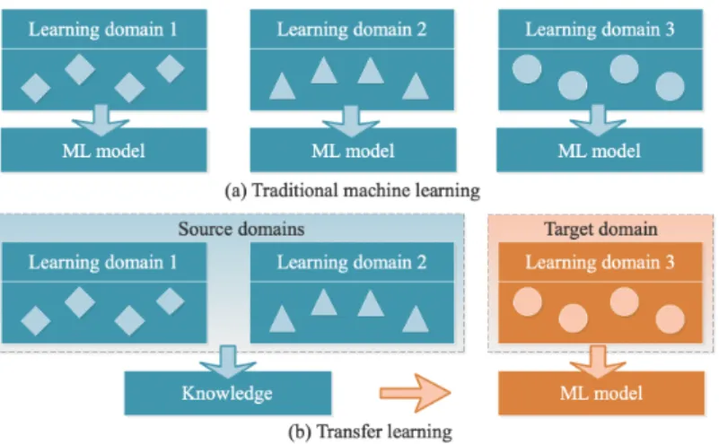
Fig. 2.4 illustrates the difference between traditional machine learning and transfer learn-ing. The traditional ML algorithms as shown in Fig. 2.4(a) learn from a single domain for each model separately, whereas transfer learning, Fig. 2.4(b), uses the knowledge gained from multiple source domains to improve learning in the target domain.

Different knowledge can be transferred across tasks and domains [9]:

• Instance transfer: Labeled data are modified and transferred to the target domain.

• Feature representation transfer: A new feature space is constructed to capture all do-mains.

• Parameter transfer: Parameters learned during training in the source domain are trans-ferred to the target to bootstrap the learning process.

(23)

2.4. Clustering 11

Figure 2.4: Traditional machine learning and transfer learning.

• Relational knowledge transfer: This approach deals with domains where there is a rela-tionship among the data and the knowledge transferred is the relarela-tionships.

In the energy forecasting with smart meter data, there is a single task (energy forecasting), but there are different domains: smart meters are considered different domains because they differ is energy consumption patterns and marginal probability distributions. SBCTL proposed here transfers weights and hyperparameters learned on the source domain (meter) to improve learning on the target domain. Thus, SBCTL belongs to the category of parameter transfer approaches.

2.4

Clustering

Machine learning algorithms build a mathematical model based on sample data, known as ”training data”, in order to perform tasks or make predictions without being explicitly pro-grammed. Machine learning approaches can be broadly classified into three categories: super-vised learning, unsupersuper-vised learning, and semi-supersuper-vised learning. In supersuper-vised learning, both inputs and desired outputs or labels are known. In unsupervised learning, the algorithm builds a mathematical model from a set of data which contains only inputs and no desired

(24)

output labels. Semi-supervised learning combines unsupervised and supervised approaches. Clustering belongs to the unsupervised learning as there is no known output class labels. Clustering discovers patterns in the data set and groups the samples into categories. Different methods have been developed to enable unsupervised clustering, but the clusters are identified in ways which are rarely stable [18]. Centroid-based clustering is a type of clustering algorithm whose cluster centers are represented by a center in the geometric space. This type of clustering algorithms is widely studied for energy load profiling, which refers to the classification of load curves or consumers according to electricity consumption behaviors [1]. In contrast to centroid-based clustering, density-based clustering identifies dense groups of points and uses sparse areas for separation. This thesis uses K-means algorithm, which belongs to centroid-based clustering.

The K-Means method was selected because it is one of the most prevalent technique for electricity smart meter consumption clustering [18]. K-Means partitionsnobservations intok clusters. The algorithm is initialized with randomly assigning k observations as cluster cen-troids (µ) and proceeds in alternating two steps:

• Assign step: Assign each of thenobservations to the closest cluster centroid based on the given distance measurement, where the Euclidean distance is often used.

S(_it)= xp : xp−µ( t) i 2 _≤ xp−µ( t) j 2_∀ j,1≤ j≤k (2.6)

wherexp represents the observations and each xp is assigned to the setS(t) according to

the Euclidean distance. The iteration step is denoted bytandistands for clusters index.

• Update step: Calculate the new centroids of the observations in the new clusters.

µ(t+1) i = 1 |S(_it)| X xj∈S_i(t) xj (2.7)

(25)

2.4. Clustering 13

and observations are not re-assigned any more. Due to random initialization of the K-Means algorithm, there is no guarantee that the algorithm will find the the optimal solution. Thus, it is preferred to rerun the K-means with different random initialization and select the clustering that produces the best evaluation performance [18].

A very challenging task in clustering has invariably been to select the right number of clusters [18]. When the ground truth for the desired output labels is unavailable, the best number of clusters is difficult to find. To determine the optimal number of clusters, indices like Dunn Index (DI) or Davie-Brown Index (DBI) are commonly used [1]. These indices usually measures the intra-cluster distance and the inter-cluster distance to evaluate a clustering algorithm.

When the clustering algorithm is used as a part of another task, the accuracy or performance of the overall task can be used for the clustering evaluation. In other words, the clustering is better if it improves the accuracy or performance of the overall task. Application-oriented metrics like the forecasting accuracy provide a way of determining a number of clusters based on the application-specific context [1].

(26)

Chapter 3

Related Work

The Related Work chapter is divided into three sections: the first section discusses energy forecasting, the second one reviews transfer learning, and the last one deals with load profile clustering.

3.1

Energy Forecasting

This section discusses generic sensor-based forecasting approaches and deep learning ap-proaches.

3.1.1

Sensor-based forecasting

Machine learning approaches have been used extensively for sensor-based energy forecasting [19]; examples include fuzzy Bayesian [20], support vector machine (SVM) [21], neural net-work [4] and ARIMA [22]. Tanget al. [20] were interested in predicting energy on an annual basis and they proposed probabilistic energy forecasting based on fuzzy Bayesian theory and expert prediction. Grolingeret al. [7] combined local learning with support vector regression (SVR) to reduce computation time while maintaining forecasting accuracy. The presented local SVR approach is compared to traditional SVR and to deep neural networks with an H2O

(27)

3.1. EnergyForecasting 15

chine learning platform for Big Data. The comparison of algorithms has also been conducted [4]; algorithms considered were Multiple Regression (MR), Genetic Programming (GP), Ar-tificial Neural Network (ANN), Deep Neural Network (DNN), and Support Vector Machine (SVM). Artificial Neural Network achieved better accuracy than the remaining five algorithms. Several algorithms were combined to form ensemble learning models. Liet al. [23] pro-posed teaching-learning based optimization with artificial neural network for hourly energy prediction. This optimized algorithm is combined with artificial neural networks (ANNs) and applied to hourly electrical energy prediction. The result shows improved performances in terms of convergence speed and prediction accuracy.

Khairalla et al. [24] investigated Stacking Multi-Learning Ensemble (SMLE) model and combined Support Vector Regression (SVR), neural network, and linear regression learners. This ensemble architecture consists of four phases: generation, pruning, integration, and en-semble prediction task. The evaluation of the proposed model was conducted to comparing with unique benchmark techniques. The result reveals that the ensemble model is an encourag-ing methodology for complex time series forecastencourag-ing. Baesmatet al. [5] proposed the weighted combination of ARIMA and RELM for city-level energy forecasting. This method not only combines the landconsumption method and curve fitting based on a generalization method, but also takes into account the saturation.

Khairalla et al. [24] investigated Stacking Multi-Learning Ensemble (SMLE) model for short-term energy forecasting. They combined Support Vector Regression (SVR), neural net-work, and linear regression learners into an ensemble model which follows the four phases process: generation, pruning, integration, and ensemble prediction task. The experiments show that the proposed SMLE achieves better forecasting accuracy than each of the individual learn-ers and better than the classic ensemble models. They do note that evaluation on other data sets are needed. Baesmatet al. [5] proposed the weighted combination of ARIMA and RELM for city-level long-term energy forecasting. This method combines the landconsumption method and curve fitting based on generalization method, while also taking into account the saturation

(28)

16 Chapter3. RelatedWork

of subscribers.

3.1.2

Deep Learning Approaches

In recent years, recurrent neural networks have gained popularity in forecasting because of their ability to capture time-dependencies. Han et al. [25] proposed wind and photovoltaic power generation prediction based on the copula function and LSTM network. They explored extracting the key meteorological factors that affect power generation and investigated the long-term dependencies and tendencies present in the limited data samples. In their experiments, the proposed approach outperformed the persistence model and the support vector machine.

Jiaoet al. [26] designed multiple sequence LSTM RNN for non-residential load forecast-ing usforecast-ing multiple correlated sequence information. The daily load curves of non-residential consumers are classified and then the Spearman correlation coefficient is used to investigate the time relations with multiple time series. The proposed approach was evaluated on a data set containing energy consumption data from 48 non-residential customers. Bouktifet al.[27] also used LSTM for energy forecasting but they combined it with genetic algorithm (GA) to find optimal time lags and a number of layers for the LSTM model.

Zheng et al. [28] combined similar days (SD) selection, empirical mode decomposition (EMD), and LSTM neural networks into a prediction model named SD-EMD-LSTM for short-term load forecasting. To calculate the similarity between historical and forecasting days, the extreme gradient boosting-based weighted K-means algorithm was used. Then, the decompo-sition of the SD load was using the EMD method with numerous intrinsic mode functions and residuals. Here, LSTM S2S networks were employed to forecast each function and residual. The forecasting values were firstly produced from each LSTM model, and then passed through a series reconstruction phase to obtained the forecasting results. The data set used was in one-hour interval, and the model was tested to forecast the next 24 one-hours (day-ahead) and 168 one-hours (week-ahead). The results showed the SD-EMD-LSTM model achieved an average MAPE of 1.08% and 1.59% for day-ahead and week-ahead forecasting respectively.

(29)

3.2. TransferLearning 17

Zheng et al. [28] combined similar days (SD) selection, empirical mode decomposition (EMD), and LSTM neural networks into a short-term forecasting model name named SD-EMD-LSTM. To evaluate the similarity between historical and forecasting days, the extreme gradient boosting-based weighted k-means algorithm was used. Then, EMD was applied to decompose the SD load into intrinsic mode functions and residuals, and a separate LSTM was employed to forecast each intrinsic mode function and residual. After the forecasting values are obtained from each LSTM, a reconstruction step merges them to obtained the final forecasting results. The evaluation was carried out with hourly data on the task of forecasting the next 24 hours (day-ahead) and 168 hours (week-ahead). The results showed the SD-EMD-LSTM model achieved an average MAPE of 1.08% and 1.59% for day-ahead and week-ahead forecasting respectively.

Standard LSTM was compared to Sequence to Sequence (S2S) architecture [29] and on one-minute time-step resolution datasets, S2S architecture performed better. Similarly, in ex-periments performed by Sehovacet al. [8], S2S RNN also outperformed standard LSTM.

As can be seen, use of NN-based solutions has been quite popular [7,21-26] and recently S2S RNN provided increased prediction accuracy [8, 29]. Nevertheless, all reviewed NN ap-proaches focus on building a prediction model for a specific building or a specific aggregated load using historical data from that same building or the same aggregated load. In contrast, our work aims to reduce computation needed to create prediction models for a large number of smart meters taking advantage of transfer learning.

3.2

Transfer Learning

This section discusses feature augmentation transfer learning, pre-trained NNs, and transfer learning in energy forecasting

(30)

3.2.1

Feature Augmentation Transfer Learning

Because of transfer learning objective to use knowledge across tasks or across domains, the concept has been applied in different domains and for different tasks [30, 31, 32, 33, 34, 35, 36]. For visual recognition, Zhuet al. [30] proposed a weakly-supervised cross-domain dictio-nary learning method. Without using any prior information, this method learns a reconstructive, discriminative, and domain-adaptive dictionary pair and the corresponding classifier parame-ters. In Natural Language Processing (NLP), Hu et al. [31] improved mispronunciation de-tection with a deep neural network trained acoustic model and transfer learning based Logistic Regression classifiers. To extract useful speech features, a neural network with shared hidden layers was first pre-trained with data pooled from different phones. Then, a phone-dependent, 2-class logistic regression classifiers were trained for mispronunciation detection.

In software engineering, Ma et al. [32] addressed cross-company software defect predic-tion and proposed Transfer Naive Bayes algorithm which used informapredic-tion from all the cross-company data for training. The classifier is built by weighting the instances of the training data according to the target set. Namet al. [33] applied a transfer learning approach, Transfer Component Analysis (TCA), to map data from the source and target sets into a single feature space. Moreover, they proposed an approach for selecting an appropriate normalization for a source-target pair. For handwritten digit recognition, Hsseinzadeh et al. [34] proposed large margin domain adaptation method, which is able to learn the connection between training and test data sets. The approach adapts the parameters of the classifier using a few or even no labeled training samples from the target data set.

In contrast to domain-specific solutions, the work of Li et al. [35] aimed to develop a transfer learning model for a variety of applications and presented augmented feature repre-sentations for domain adaptation. Similarly, Mozafari et al. [36] were interested in transfer between different domains and proposed a SVM-based model-transferring method for hetero-geneous domain adaptation. These works [30, 31, 32, 33, 34, 35, 36] focus on modifying feature space to make source and target domains more similar whereas our work belongs to the

(31)

3.2. TransferLearning 19

parameter transfer category as it does not augment features, but transfers model parameters.

3.2.2

Pre-trained NN Transfer Learning

Parameter transfer is often found associated with model-transfer and pre-trained neural net-works in computer vision [9]. Krizhevsky et al. [37] trained AlexNet, a large, deep con-volutional neural network (CNN) for classifying ImageNet data set consisting of 1.2 million pictures. It is extremely computationally expensive and time-consuming to train such a neural network with 650,000 neurons and 60 million parameters; nevertheless, once such network is trained, it is a good foundation for other image classification problems. For example, a pre-trained AlexNet [37], another deep CNN architecture, was used to detect pathological brain in magnetic resonance images (MRI). Similarly, Menegola et al. [38] used neural network pre-trained on ImageNet data set to develop a deep learning approach for melanoma screening. These parameter-transfer approaches are different from SBCTL as they are dealing with classi-fication issues rather than forecasting; moreover, image recognition problems are very different from energy forecasting.

3.2.3

Transfer Learning in Energy Forecasting

In the energy domain, transfer learning is in its early stages with a very few studies addressing different problems. Mocanu et al. [39] and Grubinger et al. [40] applied transfer learning methodologies to provide prediction models for buildings with limited historical data by using data from other similar buildings with rich data sets. The cross-building energy forecasting method Hephaestus [41] shared the same main objective; it improved the energy prediction accuracy of the target building by merging and adjusting data from several other similar source buildings. Unlike solving the limited data issue for target buildings [39, 40, 41], our work aims to reduce computation needed to train prediction models for a large number of buildings.

(32)

3.3

Load Profile Clustering

Load profile clustering has been studied for different purposes [42, 43, 44, 45]. Cerneet al.[42] divided the problem of short-term load forecasting into sub-problems: forecasting the average daily load, the amplitude of the load, and its shape. Each problem is solved separately using an adaptive TakagiSugeno fuzzy model. To build models, a combined membership function based on Gustafson-Kessel clustering and recursive weighted least mean squares was proposed. The model was tested on the real data obtained from a Slovenian energy distribution company. On this data set, the developed forecasting approach outperformed original Gustafson-Kessel and SARIMA, especially for the start of the week and for the winter.

Wanget al. [43] proposed an weighted ensemble approach for forecasting aggregated load based on hierarchical clustering. Hierarchical structure of consumers is determined according to their energy consumption patterns and multiple forecasts are obtained by varying the number of clusters. In the ensemble stage, multiple forecasts are combined to form the final forecast.

Parket al. [44] presented a load profiling methodology based on image processing technol-ogy. Data collected by smart meters are represented as load image profiles in two dimensions and modified by image processing techniques, filtering and thresholding, to reduce sensitiv-ity. According to DaviesBouldin index, the proposed approach achieved better clusters than standalone K-means, fuzzy K-means, and expectation maximization algorithm

For clustering large data sets, Zhanget al. [45] proposed an incremental clustering algo-rithm by fast finding and searching of density peaks based on K-mediods. They defined cluster creating and cluster merging operations to integrate the current pattern into the previous ones for the final clustering output. To update the cluster centers according to the new arriving samples, K-mediods is employed.

Wile the aforementioned works [42, 43, 44, 45] demonstrated various degrees of success in their respective clustering goals, our work differs as the objective is not the load clustering itself, but enabling large scale energy forecasting. Moreover, the measure of the success in our work is not the quality of the formed clusters, but the accuracy of the forecasting models

(33)

3.3. LoadProfileClustering 21

(34)

Chapter 4

Cluster-Based Chained Transfer Learning

This chapter describes the Cluster-Based Chained Transfer Learning (CBCTL) approach for building neural network-based forecasting models for a large number of meters by applying clustering and transfer learning.

4.1

Overview

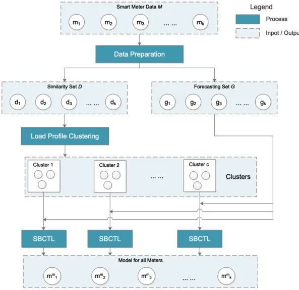
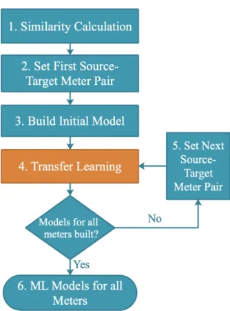
The overview of the CBCTL process is shown in figure 4.1. Starting with the smart meter data, theData Preparationprocess transforms the original data set into similarity set and forecasting set. Next, the Load Profile Clusteringgroups the meters in the similarity set in into different clusters based on their load profiles.

For each formed cluster, theSimilarity-Based Chained Transfer Learning (SBCTL) is ap-plied with the meters within that cluster. SBCTL uses the similarity set to determine the trans-fer path and the forecasting set to train the neural network models. The complete CBCTL approach is given by Algorithm 1 and the details of each stage are described in the following subsections.

(35)

4.2. DataPreparation 23

Figure 4.1: The CBCTL algorithm.

4.2

Data Preparation

The smart meter data typically contain energy readings such as consumption and demand, and the corresponding date and time. If the reading intervals are different, all smart meter data are processed to make intervals between the readings the same. In the case of energy consumption, meters with finer reading granularity are converted to a coarser granularity by adding the consumption readings.

Whereas feature selection is often considered in energy forecasting studies [1], SBCTL does not include it, as SBCTL is primarily designed for forecasting using smart meter data

(36)

24 Chapter4. Cluster-BasedChainedTransferLearning

Algorithm 1CBCTL

1: Input: Set Mconsisting of all meter data, initialization 2: Output: Models for all meters

//Data Preparation

3: D←transform1 (M)//similarity set

4: G←transform2 (M)//forecasting set (training) 5: D←normalization(D)

//Load Profile Clustering 6: C ←clustering(D)

7: forc in range(C)//for each cluster

8: // This process occurs within the current clusterc and all operations are preformed with meters belonging to the current clusterc

//SBCTL

9: L(di,dj)←similarity (di,dj), for alldi,dj ∈D,i, j∈k,i< j

10: T ← M//initialize target set 11: S ← {}//initialize source set

12: ifinitialization==A//From the most similar pair 13: (p,q)← arg min

i,j

L(di,dj), f or di,dj ∈D,i< j

14: else ifinitialization==B//From the center 15: dcenter ←mean(di), fordi ∈D

16: p←arg min i L(di,dcenter), fordi ∈D 17: q←arg min i L(dp,di), fordi ∈D,i, p 18: mm

p ←train initial model formpwithgpdata

19: S =S S

{mp} //add to source

20: T =T/S //remove from target

21: whileT , {}do 22: mm q ←transfer learning (m m p) withgq data 23: S =S S_{ mq} //add to source

24: T =T/S //remove from target

25: ifT _, {}

26: (p,q)← arg min

i,j

L(di,dj), f or mi ∈S,mj ∈T

27: Return: Models for all meters{mm₁,mm₂...mm_k}

with limited number of features; in experiments we used only seven features. Nevertheless, when working with more features, SBCTL could be augmented by adding feature selection

(37)

4.2. DataPreparation 25

step.

Let us denote this meter data asm1,m2, ...,mk ∈ M, where M is the set of all meters andk

is the number of meters. These data are processed into two data sets: the similarity setDand the forecasting setG. Meterndata inDis denoted asdn,dn ∈D, and the same meter data inG

is denoted bygn,gn ∈G. Although bothdnandgn belong to the same meter, they are different

in the number of features and time spans.

For simplification, in the Algorithm 1,Grefers to only the training part of the forecasting set. The approach starts with data preparation, specifically by creating sets D andG, lines 3 and 4.

Similarity setDis created for clustering and for the calculation of similarities among energy consumption patterns recorded by different meters (line 3). It contains only energy consump-tion readings without any addiconsump-tional features because similarity is concerned solely with usage patterns. This similarity set is used to group the meters that share similar usage patterns and, consequently, to improve transfer learning accuracy by applying SBCTL within each cluster individually. To capture quarterly and monthly patterns, Dset must contain at least one year of energy readings. Each meter datadnmust start at the same date/time to ensure alignment of

temporal patterns.

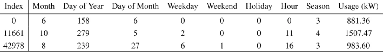
Forecasting set G, in addition to energy readings, contains other features generated from date and time such as day of the year, and weekday/weekend (line 4). Data pre-processing for this set depends on the type of the forecasting model used. As Sequence-to-Sequence (Seq2Seq) RNNs [8] have shown great results in energy forecasting for individual smart meters; they are used in SBCTL to build the initial model as well as to refine transferred models.

To enable the use of Seq2Seq RNN, data is prepared applying the sliding window tech-niques proposed by Sehovac et al. [8]. The illustration of the sliding window technique is shown in Figure 4.2. One input sample consists of a f ×T matrix where f is the number of features andT is the length of the input sequence or the number of time steps in a window. The energy readings for all time steps within a single window belong to a single sample. If the input

(38)

Figure 4.2: Sliding window technique.

sample ends at timet, the corresponding target sequence consists of time stepst+1 to t+N where N is the length of the output sequence. This way, T time steps are used to predict the nextNtime steps ahead. The next sample is generated by sliding the window for one time step and the same process keeps repeating. Different values of N result in forecasting a different number of steps ahead and thus correspond to different forecasting horizons.

The forecasting set is divided into training and test sets: first 80% of data is assigned for training and the last 20% for testing. This way, older data is used to train the model, and newer (test) data is used to evaluate and compare models. To capture monthly and quarterly patterns, the training set must contain at least one year of data; thus, the forecasting setG contains at least 15 months of data.

4.3

Load Profile Clustering

When knowledge is transferred from the source to the target domain, it is to expect that success will be higher if the two domains are more similar. Moreover, our previous work [46] demon-strated that the accuracy of forecasting is higher if the transfer occurs between more similar meters. In addition to accuracy, higher similarity of the meters requires fewer training epochs after the transfer what reduces the training time.

Consequently, the main idea behind load profile clustering is to group meters according to the similarity of their load profiles and then perform transfer only within each cluster. This will ensure that transfer occurs among highly similar meters, but it also raises questions about how

(39)

to cluster and how many clusters to use. As the number of cluster increases, the computation will also increase and the benefit of the CBCTL will decrease.

There ate two main categories of load profile clustering approaches: Direct Clustering and Indirect Clustering [1]. Direct Clustering is conducted on the smart meter data directly, while in Indirect Clustering, new features are engineered before clustering is applied.

Both Direct Clustering and Indirect Clustering have been considered in this study and each uses data from similarity set D. For both approaches, if meters differ in reading frequencies, meter data with lower intervals are aggregated. Since the actual values of energy consumption for meters differ significantly, all values from similarity set D are first scaled to bring them within the same range. Min-max normalization is performed for each meter separately bringing each meter’s value into the [0,1] range (line 5 in Algorithm 1):

˜

x= x−xmin xmax− xmin

(4.1) wherexstands for the reading value, xminfor the minimum, andxmaxfor the maximum reading

value.

After normalization, similarity setDdata is transformed differently for direct and indirect clustering (line 6 in Algorithm 1).

Direct Clustering does not further transform the readings, but directly uses energy con-sumption values. The total number of features for each meter is: 365(one year) * 24 (hours a day) * (readings per hour). An example of a sample for direct clustering is given in Fig. 4.3. Each energy reading is treated as a feature in the K-means clustering; therefore, samples for all meters must start at same date and time.

As the number of features is high, there is a possibility of encountering the curse of di-mensionality which refers to decrease in the algorithm ability as the didi-mensionality increase [47]. Moreover, similarity-based metrics upon which many machine learning models includ-ing K-means are built, breakdown in a high-dimensional space. Consequently, this study also considers an indirect clustering with a fewer number of features.

(40)

Figure 4.3: Direct Clustering seasonal profile.

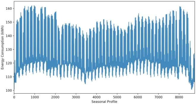
Indirect Clustering groups the meters using generated features rather than energy read-ings directly. Here meaningful representations of smart meter patterns need to be extracted. Using a singly daily profile to characterize a smart meter is not sufficient as it does not capture differences among days in the week nor it can represent seasonal changes. To capture daily loads patterns, and day of week and seasonal changes, the new seasonal profile is constructed. For each houri, day of the week j, and the seasonk, the average is calculated as follows:

xi,j,k = PN n=1(x n i,j,k) N (4.2)

whereNis the number of readings for houri, day of the week j, and the seasonk. For example, the new profile for 1:00 am on Monday in winter is calculated as the mean of all N readings at 1:00 am for all Mondays in winter. By reducing the number of features, the profile is more generic and the impact of the noise or anomalous samples is reduced.

For Indirect Clustering, the total number of features is: 4(seasons) * 7(days a week) * 24 (hours a day) = 672. The example of the seasonal profile is shown in Fig. 4.4. From left to right, the data samples are organized from winter to fall. Within each season, samples are

(41)

Figure 4.4: Indirect Clustering seasonal profile.

organized from Monday to Sunday. From the figure, it can be observed that for this specific sample, the energy load is higher during the weekdays than during the weekends. Moreover, there are some variations among seasons.

After the data is prepared according to direct or indirect approach, K-means clustering is applied with Euclidean distance as the distance metrics. Euclidean distance between samplei and sample jis calculated as follows:

LEucl(di,dj)= v t _N X t=1 (xt i −x t j)2 (4.3)

whereNstands for the number of features. Note that in direct clustering, the number of features is equal to the number of time steps whereas in the indirect clustering, it is 672.

However, the optimal number of clusters for K-means is difficult to determine. The main objective of this thesis is to build forecasting models for many meter significantly faster than traditional ML training while achieving comparable accuracy. As part of this objective, the role of K-means is to groups meters with similar usage profiles in order to maintain high accuracy.

(42)

Consequently, the application-oriented metrics are considered when analysing different number of clusters.

The outcome of the clustering algorithm is the class label for each meter, denoted asc. Note that the clustering is required only when dealing with a large number of meters. Otherwise, SBCTL can be applied directly without clustering.

4.4

Similarity-Based Chained Transfer Learning

Similarity-Based Chained Transfer Learning (SBCTL) is an approach for building neural network-based models for many meters by taking advantage of already trained models through transfer learning. The first model is trained in a traditional way whereas all other models transfer knowledge from the existing models in a chain-like manner according to similarities between energy consumption profiles.

With CBCTL, clusters are formed using K-means and then SBCTL is applied within each cluster individually as illustrated in Fig. 4.5. Within each cluster, the initial meter is selected and train using the traditional approach. Then, knowledge is transferred to remaining meters within that cluster. SBCTL that happens within each cluster is illustrated in Fig. 4.6 and details of each stage are described in the following subsections.

4.4.1

Similarity Calculation

The Similarity-Based Chained Transfer Learning (Fig. 4.6) starts with similarity calculation which gives a numeric value to similarities between each possible pair of meters within the cluster. Here, we are interested in energy patterns and not in the actual values of energy con-sumption, therefore, all values from similarity data setDneed to be scaled to bring them to the same range. The min-max normalization was performed in load profile clustering (Subsection 4.3) and similarity calculation continues using this scaled data.

(43)

4.4. Similarity-BasedChainedTransferLearning 31

(line 9, Algorithm 1); four different metrics are considered. Euclidean, Cosign, and Manhattan distances between meteriand jare calculated as follows:

Figure 4.5: Chained transfer learning.

(44)

32 Chapter4. Cluster-BasedChainedTransferLearning LEucl(di,dj)= v t _N X t=1 (dt i −d t j)2 (4.4a) LCosign(di,dj)= 1− PN t=1(d t id t j) q PN t=1(d t i)2 q PN t=1(d t j)2 (4.4b) LManh(di,dj)= N X t=1 |(dt_i −dt_j)| (4.4c) f or di,dj ∈D,i< j (4.4d)

Note that equation 4.4a is the same as equation 4.3 used in clustering. The fourth metrics considered is Dynamic Time Warping (DTW) distance [48]. DTW was selected because it is capable of measuring similarity between the two temporal sequences which may vary in speed. A well known example of a DTW application is automatic speech recognition where DTW is capable of handling different speaking speeds. In energy data, DTW could potentially capture peak shifts or prolonged peak periods. To control how much the sequences can be ”warped” for the comparison calculation, a locality constraint referred to as thewindowis commonly added. In our work, experiments consider different window sizes in order to examine their impact on the forecasting accuracy.

Forknumber of meters within the cluster, the outcome of the similarity calculation is ak∗k upper oblique matrix; this similarity matrix is denoted as Sk∗k

im . The lower the distance value

between two meters, the more similar are the meters.

4.4.2

Set First Source-Target Meter Pair

The main idea behind SBCTL is to use a similarity measure to determine the source and target meters for the transfer process. To start with, none of the meters have an associated prediction model. Therefore, as indicated in lines 10 and 11, Algorithm 1, all meters belong to the target set T and the source set S is empty. Throughout the process, the target set will always have

(45)

only the meters that do not yet have the corresponding prediction model and the source set will contain meters with an already trained model. Two different initialization techniques are considered:

InitializationA:Starting from the pair of the most similar meters. As indicated in Algo-rithm 1, line 13, the two meters that correspond to the minimum value in the similarity matrix Sk∗k

im are assigned as a starting source-target pair (p,q). Either one of the two meters in the pair

can be set as the source p; experiments will evaluate switchingpandqin the first source-target pair.

InitializationB:Starting from the meter that is the closest to the center. First, the center is calculated from the similarity data set D(Algorithm 1, line 15). For each time steptin the similarity set, the arithmetic meandcentert is calculated as:

dtcenter = 1 k k X i=1 dit (4.5)

wherekstands for the number of meters andd_it is a reading from meteriat time stept.

The meter that is the closest to this center C according to selected similarity metrics is chosen as the initial meter p(Algorithm 1, line 16). The meter that is the most similar to the initial meter pis selected as meterq(Algorithm 1, line 17).

4.4.3

Build Initial Model

This step is responsible for building the first prediction model which will serve as a starting point for the transfer learning. The initial model is built for the meter that was assigned as the sourcep(line 13 or 16, Algorithm 1). As indicated in line 17, the initial model for metermpis

trained using forecasting data setgp.

SBCTL is designed for NN-based algorithms; therefore, all models, including the initial one, must be built using the same NN approach. Specifically, a Seq2Seq RNN [8] is used because of its recent success. A Seq2Seq RNN [8] consists of an encoder RNN and decoder

(46)

RNN as illustrated in Fig. 4.7. An input sequence x[1], ...,x[T] is passed through the encoder

RNN to obtain an encoded representation of the input vector referred to as the context vector (cv~). The decoder RNN extracts information from this context vector at each output time step to obtain the prediction sequence {yˆ[1], ...,yˆ[N]}. The initial input for the decoder RNN is the

context value ˆy[0]derived from the context vector.

This first model is trained in a traditional way: weights are initialized to random values and model is trained for a sufficient number of epochs ensuring that weights converge. To avoid local minimum, the process is repeated starting with a different set of random initial values referred to asseeds. The best model among all runs with different seeds is chosen for forecasting and used in the following chained transfer learning steps.

NN hyperparameters such as a number of layers and neurons, are also tuned in this step by splitting the training data into the training and validation sets; model selection is done on the validation set. After tuning hyperparameters for the initial model, they remain the same throughout the transfer learning and for all meter models. In contrast, the weights learned during the initial model training are used as a starting point for other models, but the weights do change.

The result of the training and tuning is the prediction model for meter p denoted as mmp

(Algorithm 1, line 18). Note that mp indicates meter data for the meter pandmmp denotes the

(47)

trained model for the same meter p. Because meter p now has the forecasting model, it is added to the set of source metersS, line 19, and removed from the set of target metersT, line 20. This initial model is now available for transfer learning.

4.4.4

Transfer Learning

The initial modelmm

p is used as a seed for building all other prediction models through transfer

learning. The assumption is that if the meters share some similarity, so should their trained models. Thus, if we use the initial prediction model as a starting point for building the model for the most similar meter, the training should be reduced.

The meter to transfer knowledge to is the qmeter from the (p,q) pair. Because the pair is determined according to similarities, SBCTL ensures that the transfer happens between more similar meters. As indicated in line 18, existing model mm

p trained previously for meter p

and with data set gp, is now used as a starting point for building meter q model. Model mmp

continues training, but now with the target meter datagqto obtain modelmmq. Network structure

and hyperparameters determined during training for the first meter remain the same throughout the transfer learning and for all forecasting models. The weights from the source meter model mmp are transferred to the target meterq, but they change through training with the target meter

datagq. The number of training epoch needed for the weights to converge is lower because the

training starts from the pre-trained weights.

If the two meters from the pair are very similar, the transferred model, without any training with the target meter data, may already provide reasonable accuracy: we refer to transfer with-out additional training as epoch 0. The evaluation will explore how many epochs with target data are needed to achieve comparable accuracy to traditional NN training.

The result of the training with the transferred model is the new modelmm

q, line 22. Next, as

meterqnow has the forecasting model, it is added to the set of source meters S, line 23, and removed from the set of target meters T, line 24. This additional model now is available for transfer learning.

(48)

If there are still meters that do not have a corresponding prediction model, in other words, if the target setT is not empty (lines 25 and 21), the SBCTL will proceed to Set Next Source-Target Meter Pair step. If forecasting models are trained for all meters, the SBCTL process is completed.

4.4.5

Set Next Source-Target Meter Pair

In this step, the next source-target meter pair (p,q) is selected for transfer learning. As indicated in the algorithm’s name SBCTL, the processed is chained: building the next forecasting model depends on the previously built models. In each loop of the chained process, the forecasting model will always be transferred from one meter in the source setS to one meter in the target setT.

To determine which model should be trained next, the similarity distances calculated in line 9 are used. Because the transfer needs to happen from an already trained model, we are interested in finding a meter from the target setT that is the most similar to any meter in the source setS. Thus, line 26 in Algorithm 1 finds the pair with minimum distance Lunder the constraint thatmp ∈S andmq ∈T. The model will be transferred from frommptomq.

When the next source-target pair (p,q) is set (line 26), SBCTL continues to transfer learn-ing, line 21, described in subsection 4.4.4.

4.4.6

ML Models for all Meters

This is the final output of the CBCTL process. As indicated in lines 7 and 21, the transfer learning process completes when the target set is empty T = {} for all the clusters and all meters belong to the source set S. The algorithm results are the trained ML models for all metersmm 1,m m 2...m m k.

(49)

Chapter 5

SBCTL Evaluation

This chapter focuses on evaluating SBCTL while the next chapter evaluates CBCTL. The SBCTL evaluation process is introduced first, followed by the three experiments with different data sets and, finally, the findings are discussed.

Experiments one and two consider smaller data sets consisting of 7 and 19 meters, respec-tively. A small number of meters in these two experiments allows for detailed examination of the transfer process as well as for accuracy comparison for each individual meter. On the other hand, the third data set consisting of 456 meters allows for evaluation at scale and demon-strates SBCTL forecasting accuracy and time savings with larger data. The used hardware was different for each data set and reflects the increase of data set size.

All of the experiments applied SBCTL with initializationsAand B. Also, Euclidean, Co-sine, Manhattan, and DTW distance with window size of 3, 6, 12, and 24 were evaluated. SBCTL was implemented using Python with Pandas and PyTorch libraries. GRU cells were used in Seq2Seq RNN because they achieved higher accuracy than LSTM in single meter fore-casting [8]. The hyper-parameters used for the initial model as well as for all other models were:

• Hidden dimension size=64

• Batch size=256

(50)

38 Chapter5. SBCTL Evaluation

• Epochs=10

• Optimizer=Adam

• Learning rate=0.001

• Loss function=MSE

• Encoder size=8

• Decoder size=4

5.1

Evaluation Process

To evaluate model accuracy, all three experiments use two metrics: Mean Absolute Error (MAE) and Mean Absolute Percentage Error (MAPE). The two metrics were chosen because they are frequently used in energy forecasting studies [1]. MAE and MAPE are calculated as follows: MAE= 1 N0 N0 X t=1 |yt−yˆt| (5.1) MAPE= 100% N0 N0 X t=1 yt−yˆt yt (5.2)

whereyrepresents the actual value, ˆyis the predicted value, N0 stands for the number of test

set samples, andt indicates reading time steps. Time consumed for each training epoch was also recorded for the evaluation purpose.

For each meter in each experiment, SBCTL was compared to the traditional machine learn-ing:

• Traditional training: For each meter, an individual RNN model was trained using that meter training data. The process was repeated with 10 seeds and the model with the

(51)

5.2. ExperimentOne 39

best MAPE was selected for comparisons. As a large number of models from the two experiments converged around the 10th epoch, the comparison was carried out with 10 epochs. Moreover, comparing all meters using the same number of epochs provides the ability to compare across meters. For each epoch, the model was tested on the test set and accuracy was recorded. This will enable observation of MAPE/MAE reduction through epochs.

• SBCTL:The models were built using SBCTL approach. In each experiment, the first model was built using the traditional approach. All other models were built using SBCTL transfer learning and only trained for 5 epochs because the training starts from the pre-trained weights. For each epoch, including 0 epoch (no training on target), the models were tested on the test set and accuracy was recorded.

5.2

Experiment One

This experiment was performed on MacBookPro with 2.9 GHz Intel Core i7 processor and 16 GB LPDDR3 memory.

5.2.1

Data set

Experiment one used a private data set from seven real-world meters measuring commercial buildings energy consumption in 15 min intervals. This data set, as well as data sets in remain-ing experiments, consists of readremain-ing date/time with corresponding energy