Measuring Market Damage of Automobile Related Carbon Tax by Dynamic Computable General Equilibrium model

(1)

27-30 August 2003

European Regional Science Association

The 43rd European Congress

University of Jyväskylä, Jyväskylä, Finland

Shinichi MUTO,

Department of Civil Engineering and Urban Design, Osaka Institute of Technology (Ohmiya 5-16-1, Asahi-ku, Osaka 535-8585, JAPAN)

E-Mail : [email protected]

Hisa MORISUGI,

Department of Civil Engineering, Graduate School of Information Sciences, Tohoku University

(Aoba, Aoba-ku, Sendai, 980-8579, JAPAN)

and Taka UEDA

Department of International Development Engineering, Tokyo Institute of Technology (Ookayama 2-12-1, Meguro-ku, Tokyo 152-8552, JAPAN)

Measuring Market Damage of Automobile Related Carbon Tax

by Dynamic Computable General Equilibrium model

Abstract

This paper tries to evaluate the market damage of automobile related carbon tax to be imposed as a control of CO2 emissions. Japanese Ministry of Transport set up a target of the GHG emission level of transport sector at 2008 to 2012 as 17% increasing level from 1990 level. In order to comply with this target, Ministry of Transport has been investigating the feasibility and acceptability of automobile related carbon tax. But the economic damage of those policies is not elucidated enough. Hence we evaluate its influence on the market economy by applying the dynamic computable general equilibrium (DCGE) model. The model has characteristics of explicit formulation of the automobile related industrial and transport sector’s behavior and household travel behavior.

With this model, we identify the automobile related carbon tax levels needed to accomplish the regulatory target of CO2 emissions at transport sector for two cases with respects to the price elasticity in fuel demand. In the lower elasticity case of 0.1, the necessary carbon tax is 112[thousand yen/tC] and the associated market disbenefit is 1,810[billion yen/year]. In higher elasticity case of 0.3, the necessary carbon tax is 119[thousand yen/tC] and the market disbenefit is 2,490[billion yen/year]. In addition to above analysis, we also evaluated the subsidy policy for clean energy vehicle.

(2)

1. Introduction

Issues of external diseconomies caused by automobiles have been a more serious problem. Especially, the damages suffered by Green House Gas (GHG) emissions are recognized as global warming and, at the Kyoto Protocol (COP3), the regulatory targets of GHG emissions were specified for signatory countries. The target for Japan is 6% reduction from 1990 level in the period 2008-2012, and the target of transport sector was set up by Ministry of Transport, which is 17% increasing from 1990 level. Ministry of Transport has estimated to grow the GHG emissions by 40% if no policies were performed. To reduce GHG emissions exhausted by automobiles is, therefore, an important task because the emissions of them occupy 90% of all transport sectors.

On the other hand, the policies based on market mechanism, like an environmental tax, have been proposed in order to regulate GHG emissions. The impacts exerted by executing these policies, however, are not elucidated enough. It is well known that these policies raise commodity prices through the increase of automobile user’s costs, and, as result, the huge welfare loss, what is called deadweight loss, is possible to be generated. Those recognition leads to need to evaluate synthetically the economized environmental policies by calculating the deadweight loss due to executing these policies.

In this paper, we focus on the carbon tax policy imposed only to automobiles, and evaluate it with the dynamic computable general equilibrium (DCGE) model. In this DCGE modeling, the economic behaviors of household and industries, and the mechanism of market are formulated by mathematical programming, and the dynamic path is calculated. Hence the model allows us to grasp the change of agents’ behaviors due to introduce the carbon tax, and measure the damage given to market economy, what is named by us the market disbenefits, by utilizing the concept of equivalent variation. Note that we ignore the social benefits generated by reducing GHG emissions, in other words we assume here that their benefits are not occurred in the studied period. The CGE approaches have been developed to evaluate economic impacts with introducing tax policy or international trade policy, which are surveyed by Shoven and Whalley (1984). Jorgenson and Wilcoxen (1990) and Bergman (1991) applied the CGE model for the environmental policy evaluation. Such approach had been more exquisite by Ballard and Medema (1993) and Goulder et al (1999), and applied to the transport environmental problems by Borger and Swysen (1998) or Mayeres (2000). Recently, in the magazine of the review of urban & regional development studies (RURDS), a special edition on the CGE approach compiled in 2003. In there, Roson (2003) or Rana (2003) computed the economic impact of CO2 emission controls.

The DCGE model of this research follows those previous CGE approaches in principle. Our model explicitly formulates, however, the automobile related industrial or transport sector’s behavior and household travel behavior. Especially, the travel behavior for private tips of household is formulated by the probability choice paradigm shown by McFadden (1981).

(3)

2. Partial analysis

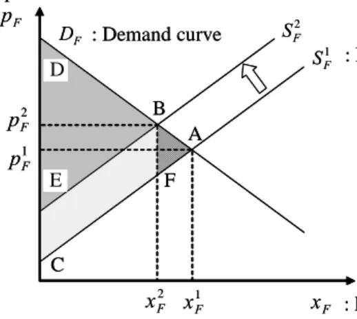
In this section, before building the theoretical model, we show the economic impacts of the carbon tax in the framework of partial equilibrium analysis on the automobile fuel market. In this context, suppose that the carbon tax is levied on the automobile fuel. In figure 1, the demand and marginal cost curve in the fuel market are drawn. Without carbon tax case, the pricing scheme yields to the market equilibrium point A. Levying the carbon tax equivalent to BF on fuel services moves the market equilibrium from point A to the point B through the shift of marginal cost curve.

This movement of market equilibrium point decreases the social surplus from CAD to EBD. In another word, the economic loss, CABE is generated. However the CFBE is the amount of paying the carbon tax which is equal to the government’s gain as tax revenue. Hence the government revenue CFBE is deducted from CABE, so FAB is the net economic loss due to introduce the carbon tax. This is called to deadweight loss of taxation. In this paper, we will measure this deadweight loss by using the DCGE model.

A B C D F D_F : Demand curve

S_F1 _{: Marginal cost curve}

x_F1 x_F2 p_F1 x_F : Fuel consumption p_F Fuel price E S_F2 pF 2 A B C D D F D_F : Demand curve

S_F1 _{: Marginal cost curve}

x_F1 x_F2 p_F1 x_F : Fuel consumption p_F Fuel price E E S_F2 pF 2

Figure 1. Impacts due to introduce the carbon tax

3. Structure of Dynamic Computable General Equilibrium Model 3.1Assumptions

We have the following major assumptions.

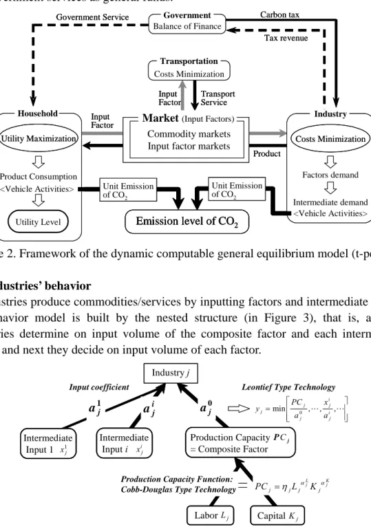
(a) An economy consists of a representative household, industries (Eight transport sectors and five other sectors) and a central government, as illustrated in Figure 2. (b) The industry provides commodities/services by inputting factors that consist of

labor and capital, and intermediate goods.

(c) The household gains income by supplying factors and consumes commodities/services provided by industries under the budget constraint.

(d) We are modeled the savings behavior of household. The savings are appropriated the investment in all, by which the next period capital stock is accumulated. The decision making of savings is assumed to be done under the myopic expectation, where people consider that the present circumstance is continuous at next period. (e) All transport services both of passenger and freight are supplied by the transport

(4)

sectors. However private automobile trips consumed by household are provided by his own.

(f) Markets are considered on each commodity, labor and capital. They are assumed to be perfectly competitive.

(g) The central government levies the carbon tax on automobile fuels, which consist of gasoline and light-oil. A part of tax revenue is appropriated the subsidy to purchasing of the clean energy vehicles, and the rest of them is done to provide the government services as general funds.

Market (Input Factors) Balance of Finance Government Transportation Costs Minimization Carbon tax Tax revenue Household Utility Maximization Product Consumption <Vehicle Activities> Utility Level Government Service Input Factor Input Factor Transport Service Product Industry Factors demand Intermediate demand Costs Minimization <Vehicle Activities> Commodity markets Input factor markets

Unit Emission of CO₂ Unit Emission

of CO₂

Emission level of CO₂ Market (Input Factors)

Balance of Finance Government Government Transportation Transportation Costs Minimization Carbon tax Tax revenue Household Household Utility Maximization Utility Maximization Product Consumption <Vehicle Activities> Utility Level Government Service Input Factor Input Factor Transport Service Product Industry Industry Factors demand Intermediate demand Costs Minimization Costs Minimization <Vehicle Activities> Commodity markets Input factor markets

Unit Emission of CO₂ Unit Emission of CO₂ Unit Emission of CO₂ Unit Emission of CO₂ Emission level of CO₂ Emission level of CO₂

Figure 2. Framework of the dynamic computable general equilibrium model (t-period)

3.2Industries’ behavior

Industries produce commodities/services by inputting factors and intermediate goods. Its behavior model is built by the nested structure (in Figure 3), that is, at first, industries determine on input volume of the composite factor and each intermediate goods, and next they decide on input volume of each factor.

Input coefficient ai_j aj

1

a0_j

Leontief Type Technology

        =min ₀ ,L, _i ,L j i j j j j a x a PC y

Production Capacity Function: Cobb-Douglas Type Technology

K j L j j j j j L K PC =η α α LaborLj CapitalKj Industry j Intermediate Input 1 x1j Intermediate Input i xij Production Capacity = Composite Factor PCj Input coefficient ai_j aj 1 a0_j

Leontief Type Technology

        =min ₀ ,L, _i ,L j i j j j j a x a PC y

Production Capacity Function: Cobb-Douglas Type Technology

K j L j j j j j L K PC =η α α LaborLj

LaborLj CapitalCapitalKKjj Industry j Industry j Intermediate Input 1 x1j Intermediate Input 1 Intermediate Input 1 x1j Intermediate Input i Intermediate Input i xij Production Capacity = Composite Factor PCj Production Capacity = Composite Factor PCj

Figure 3. Outline of industries’ behavior

At first step, the industries’ behaviors inputting the composite factor and intermediate goods are formulated as minimization of production costs under Leontief type technology constraint.

(5)

Cj c PC p x PC x j j i j i i j ji = min ⋅ +

∑

, (1a) s.t. y PC a x a j j j j i j i =         min , , 0 L L (1b)

Where, PCj: production capacity (input volume of composite factor), xj

i_{: intermediate}

goods input volume from industryi to industryj, yj: output volume, cj: unit cost of

composite factor, pi : the price of commodity i , aj

0 _{: production capacity rate}

[production capacity for the unit output], a ij( )

i _≠

0 : input coefficient in Leontief Matrix

and Cj: product cost.

Solving the programming in (1), we obtain production capacity PCj and

intermediate goods input volumexj

i_{, respectively.}

PCj =a yj j 0

(2a)

xij =a yij j (2b)

Substitution of the (2) into the (1) gives the product cost Cj in industryj,

Cj a cj j a p yj i i i j = +     

∑

0 . (3)

At second step, industries decide on input volume of each factor. The behavior is formulated as minimization of the cost for input factors under Cobb-Douglass type technology constraint. cj p L p K L Kj j L j K j = min + , (4a) s.t. PCj jLj jKj L j K =η α α = 1 (4b)

Where, Lj,Kj: labor and capital input volume, respectively, pL, pK: labor wage and

capital rent, respectively and η_j,α_L_j,α_K_j: parameters [α_L_j+α_K_j =1].

The solution of cost minimization programming for input factors in (4) yields to the input volume of each factor demand function DL_j,DK_j for unitPCj.

Labor input: D p p L j j L K j K L j j K =         1 η α α α (5a) Capital input: D p p K j j K L j L K j j L =         1 η α α α (5b) Substituting (5) into the (4), we obtain the unit cost of composite input factorcj,

cj p p j j L j K j K j L L K j K jL jL jK =    _ +_ _           1 η α α α α α α α α . (6)

3.3Price vector of products

The price [pj] of commodityj is led through the zero profit condition in industry j.

(6)

(

)

Cj a c p pj j L K a p yij i i j = +     

∑

0 , . (7)

The carbon tax and the subsidy for the clean energy vehicle are assumed to be imposed/provided on input factor costcj. So Cj is represented like this.

(

)

_{

_}

Cj a c p pj j L K j a p yj i i i j = + +     

∑

0 1 , τ . (8)

Where, τj: tax/subsidy rate.

The subsidy rate τj may be considered as negative tax.

We can have the profit of industryj from (8) as below,

(

)

{

}

πj j j j j L K τj ij i i j p y a c p p a p y = − + +     

∑

0 _, ₁ _{. (9)}

Where, πj: profit of industryj.

The (9) is linear type for yj, so the market equilibrium solutions exist under the zero

profit condition. Its condition gives the commodity pricepj,

(

)

_{

_}

pj a c p pj j L K j a pj i i i = 0 + +

∑

1 , τ . (10)

By arranging (10), we obtain a price vector of commodity,

[

]

′ = ′ ⋅ − −

p c I A 1. (11)

Where, p: price vector of commodity, c: product vector of composite factor unit cost by production capacity rate, I: unit matrix, A : input coefficient matrix and ’: transposed matrix.

3.4Behavior of clean energy vehicle product industry

In Japan, the clean energy vehicle is beginning to be diffused. Though its product price is higher than the one of general vehicles, it is expected that the accumulation of them may decrease its price by learning effects in its product industry. In this paper, we will grasp the leaning effects through the next formulation of clean energy vehicle industry’s product behavior, in which an additional fix cost is introduced. Its cost is assumed to depend on the product volume

{

∑

=₌−1

}

1 t s s s C

y of clean energy vehicle accumulated by previous period and decrease with increasing of

∑

=₌−1

1 t s s s C y . The product behavior of clean energy vehicle is described like below,

( )

CC c PC p x FC Y y x PC C C i C i i Ct C Ci C = ⋅ +

∑

+ − ⋅ min , 1 _(12a) s. t. y PC a x a C C C C i C i =       min ₀ ,_L ,_L (12b)

Where, subscriptC: clean energy vehicle product industry, FC: additional fix cost, YCt−1: accumulated volume of clean energy vehicle product

{

∑

}

− = = = 1 1 t s s s C y .

(7)

industries. But the product cost is increased by the additional fix cost.

(

){

}

( )

CC a c p pC C L K C a pCi i FC Y y i Ct C = + + +     

∑

− 0 1 1 , τ (13)

And the clean energy vehicle’s price is led as below,

(

){

}

( )

pC a c p pC C L K C a pC FC Y i i i C t = 0 + +

∑

+ −1 1 , τ (14)

From this result, even if the clean energy vehicle product industry has the same technology with another general automobile product industry, the price of them is risen up by additional fix costFC. However, as being increased the number of them, FC is decreased less and the difference of price between the clean energy vehicle and another general vehicle is gradually shortened.

In figure 4, we show the actual values of accumulated vehicles and its selling price on the case of T type produced by the Ford, and we estimate the additional fix cost function

( )

t−1 C

Y

FC based on their values. But

( )

t−1 C

Y

FC in Figure 4 is adjusted by the actual data of the clean energy vehicle’s price and the number of accumulated one of Japan in 1995.

0.0 0.2 0.4 0.6 0.8 1.0 1.2 1.4 推計値 0.0 0.2 0.4 0.6 0.8 1.0 1.2 1.4 0 5,000 10,000 推計値

The number of accumulated clean energy vehicle(1000 Veh.) Actual value of Ford T type Estimated value T h e pr ice o f c le a n e n er g y v e h ic le pC

{ }

₁ 0.108 46 . 2 ⋅ − − = t C C Y p 1 − t C Y 0.0 0.2 0.4 0.6 0.8 1.0 1.2 1.4 推計値 0.0 0.2 0.4 0.6 0.8 1.0 1.2 1.4 0 5,000 10,000 推計値

The number of accumulated clean energy vehicle(1000 Veh.) Actual value of Ford T type Estimated value T h e pr ice o f c le a n e n er g y v e h ic le pC

{ }

₁ 0.108 46 . 2 ⋅ − − = t C C Y p 1 − t C Y

Figure 4. Estimated price of clean energy vehicle

3.5Household behavior (1) Outline of model

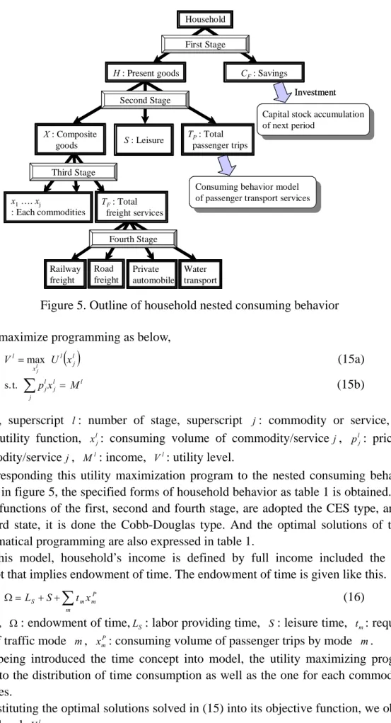
Household gains income by providing the input factors which consist of labor and capital, and determines the consuming volume of commodities/services so as to maximize his utility under the budget constraint. Hence the consuming behavior of the household should be illustrated in a nested structure, as shown in figure 5. This structure has been proposed by Shoven and Whalley(1992).

(2) Formulation of consuming behavior

At first stage, the household determines consumption levels of present goodsH and savingsCF, and, at second stage, ones of composite goods, leisure time and total

passenger trips, and, at third stage, ones of each commodity and total freight transport services, and, at fourth stage, ones of each traffic mode on freight transport. The choice models on passenger trips are formulated in more detail by using the nested logit model that will be explained at next section.

(8)

Household First Stage

H : Present goods C_F: Savings

Second Stage Third Stage X: Composite goods S : Leisure T_P: Total passenger trips Investment Capital stock accumulation of next period

x1…. xj

: Each commodities

TF: Total

freight services

Consuming behavior model of passenger transport services

Fourth Stage Road freight Private automobile Railway freight Water transport Household First Stage First Stage H : Present goods

H : Present goods CC_F_F: Savings: Savings

Second Stage Second Stage Third Stage Third Stage X: Composite goods X: Composite

goods S S : Leisure: Leisure

T_P: Total passenger trips

Investment Capital stock accumulation of next period x1…. xj : Each commodities x1…. xj : Each commodities TF: Total freight services TF: Total freight services

Consuming behavior model of passenger transport services Consuming behavior model of passenger transport services

Fourth Stage Fourth Stage Road freight Private automobile Railway freight Water transport Road freight Private automobile Railway freight Railway freight Water transport Water transport

Figure 5. Outline of household nested consuming behavior utility maximize programming as below,

( )

l j l x l _U _x V _l j max = (15a) s.t. p xl_j l_j M j l

∑

= (15b)

Where, superscript l: number of stage, superscript j: commodity or service, _Ul_:

direct utility function, xlj: consuming volume of commodity/servicej, l j

p : price of commodity/servicej, Ml: income, Vl: utility level.

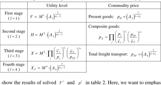
Corresponding this utility maximization program to the nested consuming behavior shown in figure 5, the specified forms of household behavior as table 1 is obtained. The utility functions of the first, second and fourth stage, are adopted the CES type, and at the third state, it is done the Cobb-Douglas type. And the optimal solutions of those mathematical programming are also expressed in table 1.

In this model, household’s income is defined by full income included the time concept that implies endowment of time. The endowment of time is given like this.

Ω =LS + +S

∑

t xm mP

m

(16) Where, Ω: endowment of time,LS: labor providing time, S: leisure time, tm: required

time of traffic mode m, P m

x : consuming volume of passenger trips by mode m.

By being introduced the time concept into model, the utility maximizing program yields to the distribution of time consumption as well as the one for each commodities /services.

Substituting the optimal solutions solved in (15) into its objective function, we obtain utility level Vl.

(9)

Table 1. Formulation of household consuming behavior

Utility maximizing program Consuming volume of commodities

(

)

₁ 1 1 1 1 1 1 1 , 1 max β σ ν β σ ν ν     ₊ ₋ = _H _H _F C H H C V F

(

1

)

s.t.p_HH+p_FC_F = p_LΩ+p_KK ≡M Present goods: H M p H H = β_σ 1 1 1∆ Savings: C

(

)

M p F H F = 1− 1 1 1 β σ _∆ Where,∆1 ( )

(

)

( ) 1 1 1 1 1 =_β −σ + −_β −σ HpH H pF First stage (l=1)

pH:present goods price, pF:saving price, Ω: endowment of time, K: endowment of

capital, M1

: full income, βH : parameter, σl : elasticity of substitution,

νl:=

(

σl−1

)

σl , V: utility level. H X S T X S TP X S P P =  + +    max , , γ γ γ σ ν σ ν σ ν ν 1 1 1 1 2 2 2 2 2 2 2 s. t.p X_X +p S p T_L + _TP _P = M2

Composite goods: Leisure:

X M p X X = γ _σ 2 2 2_∆ S M p S L = γ _σ 2 2 2_∆

Total passenger trips:

T M p P P TP = γ _σ 2 2 2_∆ Where, ( ) ( ) ( ) ∆₂=γ 1−σ2 +γ 1−σ2 +γ 1−σ2 XpX lpL TP TPp First stage (l=2)

pX : Composite goods price, pTP :Total passenger transport price,

M2

:= M1−p CF* F*,γ γ γX, l, P:parameters, H: Utility level gotten from consuming

volume of present goods.

X x T x T j j F j F j F =max

∏

⋅ , ς ς s.t. p x_j _j p T M j TF F

∑

+ = 3

(j:each commodity except automobile, fuel and freight transport)

Each commodity j: x p M j j j = ς 3

Total freight transport: X

p M F F TF = ς 3 Third stage (l=3)

pj′ : each commodity price, pTF : total freight transport price, M 3 _：

= M2− p X*X *− p TTP P* *, ς ςj, F: parameters, X : Utility level gotten from consuming

volume of composite goods. F F F j _j j j x F x X χ σ ν ν 1 1 max         =

∑

s. t. p x_j _j M j

∑

= 4 (j: freight transport)

Freight transport consumption of each traffic modej′: x M p j j j = χ_σ 4 4 4∆ Where, ∆4 ( ) 1 4 =

∑

_χ −σ j j j p Fourth stage (l=4)

pj′: freight transport price, M4:= M −

∑

_jp xj j

3 * *

, χj: parameters, XF: Utility level

gotten from consuming volume of freight transport services.

(

)

Vl V p Ml j

l l

= , (17)

The commodity/service price at the lth stage is led through transforming the result of (17) and the budget constraint equation at the same stage as below.

( )

(10)

Table 2. Specified utility level of household and commodity price

Utility level Commodity price

First stage (l=1) V = M1⋅

( )

1 − 1 1 1 ∆ σ _Present_goods:_p

( )

H = ∆2 − 1 1 σ2 Second stage (l=2) H= M2⋅

( )

2 − 1 1 2 ∆ σ Composite goods: pX p p j j j TF F j F =    _ _   

∏

_ς _ς ς ς Third stage (l=3) X M _p _p j j j F TF j F = ⋅    _ _   

∏

3 ς ς ς ς

Total freight transport: pTF =

( )

∆4 − 1 1 σ4 Fourth stage (l=4) XF = M ⋅

( )

− 4 4 1 1 4 ∆ σ

We show the results of solved Vl and pl in table 2. Here, we want to emphasis that the nested utility maximizing behaviors become to be consistent by leading the relation among prices of each stage as (18).

Next, we explain the saving behavior of household. The savings are led under the balance of returns and loss generated by investing all savings to accumulation of capital stock. The return of investment is given as capital rent dividend. Supposing the myopic expectation in this model, the household consider next period’s rent the same as present one. So such rent dividend is expressed as

I

pK (19)

Where, I : investment volume, that corresponds with accumulation of capital stock.

K

I=∆ (20)

On the other hand, the loss of investment is yielded as value of the present good consumption that has been given up by investing. This consumption is defined as the future goods CF that is formulated at first stage in table 1. Assuming myopic

expectation, the price of CF is equivalent to the present composite good’s price.

From these result, the balance equation (21) between return and loss of investment, is to be constructed.

p IK = p CX F (21)

Here assuming pI to investment price, which will be introduced in (25) at next

paragraph. Hence pII indicates the amount value of investment and implies also the

one of saving. The (21) is modified by introducing the pI. F K X I I C p p p I p _      = (22)

The coefficient of CFis defined as pF.

p p p

p F I X

K

≡ (23)

The pF can be considered as the price of future goods, CF. Obtaining the numerical F

p by (23), we can solve the utility maximize programming at the first state. The optimal solutions of its programming give also the value of future goods that implies

(11)

amount of investment from equation of (22). The investing amount is appropriated to purchasing invest goods to accumulate the capital stock. The purchasing volume of them is given as below.

j I j I j p I p x =ξ ⋅ (24)

Where, xIj : purchasing volume of investment goods, ξj : expenditure share of

investment goods.

From the definition of ξj, the investment price, pI is obtained as

∑

= j j j I p p ξ . (25)

(3) Formulation of passenger trip consuming behavior

In this section, we try to introduce the modal choice for the consumption of total passenger trips, TP (see l=2 in table 1).

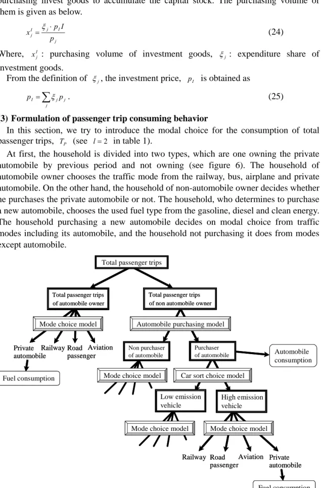
At first, the household is divided into two types, which are one owning the private automobile by previous period and not owning (see figure 6). The household of automobile owner chooses the traffic mode from the railway, bus, airplane and private automobile. On the other hand, the household of non-automobile owner decides whether he purchases the private automobile or not. The household, who determines to purchase a new automobile, chooses the used fuel type from the gasoline, diesel and clean energy. The household purchasing a new automobile decides on modal choice from traffic modes including its automobile, and the household not purchasing it does from modes except automobile.

Automobile consumption Automobile purchasing model

Mode choice model

of automobile owner Total passenger trips

Non purchaser of automobile Private automobile Railway Road passenger Total passenger trips

of non automobile owner Total passenger trips

Mode choice model Mode choice model

Purchaser of automobile Aviation Low emission vehicle High emission vehicle Fuel consumption Mode choice model

Car sort choice model Railway Road passenger Aviation Private automobile Fuel consumption Automobile consumption Automobile purchasing model

Automobile purchasing model Mode choice model

Mode choice model

of automobile owner Total passenger trips of automobile owner Total passenger trips of automobile owner Total passenger trips

Non purchaser of automobile Non purchaser of automobile Private automobile Railway Road passenger Total passenger trips

Total passenger trips

of non automobile owner Total passenger trips of non automobile owner Total passenger trips of non automobile owner Total passenger trips

Mode choice model Mode choice model Mode choice model

Mode choice model

Purchaser of automobile Purchaser of automobile Aviation Low emission vehicle Low emission vehicle High emission vehicle High emission vehicle Fuel consumption Fuel consumption Mode choice model

Mode choice model

Car sort choice model Car sort choice model Railway Road passenger Aviation Private automobile Fuel consumption Fuel consumption

(12)

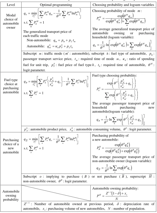
We model those passenger trips consuming behavior of household in the framework of nested logit model. The behavior model at one level is formulated as well as Miyagi(1986) like below,

      − =

∑

m l m l m l m m l m P h P q P P q l m ln 1 max θ (26a) 1 . t . s

∑

= m l m P (26b)

Where, superscript l : number of level, subscript m: traffic mode of passenger transport (example), Pml : choice probability of mode m, qm: generalized transport

price and _θl_{: logit parameter.}

The programming in (26) yields to the probability functions expressed by the logit model.

( )

∑

= m m l m l l m q q P θ θ exp exp (27) Substituting (27) into objective function of (26), we obtain inclusive expected

generalized transport price qh as logsum variable.

( )

∑

= m m l l h q q θ θ ln exp 1 (28) Corresponding this expected transport cost minimization program in (26) to the

nested transport choice behavior illustrated in figure 6, we can get the specified model shown in table 3. The optimal programming is indicated on the left side of table 3, and the logit models and logsum variables obtained by being solved its programming is done on the right side. The logsum variable is equivalent to the cost function of upper choice model. Though the automobile owning probability is not led as logit model and the logsum variable also can not be obtained, the total passenger transport price, pTP is

given by the weighted average of its probability.

3.6Government behavior

The government levies the carbon tax for CO2 emissions on automobile fuel

consumption. A part of tax revenue is appropriated the subsidy to diffuse of the clean energy vehicles, and the rest of them is done to provide the government services as general funds. When the government service is supplied, it consumes some commodities. Its government consumption is given as

[

]

j S T j G j p x =ς Ψ +Ψ . (29) Where, G j

x : volume of government consumption, ςj : expenditure share of government

consumption, _ΨT_{: tax revenue of carbon tax,}

(

)

0

≤ Ψ

ΨS S _{: subsidy for clean energy}

vehicle.

The household utility has been increased by providing the government service. The benefit of utility increasing is assumed simply to be equivalent to the amount of expenditure to government service,

[

_ΨT ₊_ΨS

]

_.

(13)

Table 3. Formulation of transport choice model on the passenger trips

Level Optimal programming Choosing probability and logsum variables

q_h m m =  −     

∑

min P m M m M m M m M mM P q 1 P P θ ln s.t. PmM m

∑

=1

The generalized transport price of each traffic mode

Non-automobile: qm= pm+p tL m Automobile: L h h F h h m p p t q ′ =κ +

Choosing probability of mode m:

(

)

(

)

+

_∑

(

)

= ′ m m M h m M m M M m q q q P θ θ θ exp exp exp

The average generalized transport price of automobile owning or purchasing household (logsum variable):

(

)

(

)

      + = ′

∑

m m M h m M M h q q q θ θ θ ln exp exp 1 Modal choice of automobile owner

Subscript m: traffic mode (m′: automobile), subscript h: fuel type of automobile, pm:

passenger transport service price, tm: required time of mode m, κh: ratio of spending

fuel for unit trip, phF: fuel price of fuel typeh, th: required time of automobile, θ

M : logit parameter.         −       + =

∑

′ h S h S h S h h h m h A S h P B q P P x p P q _S h ln 1 min θ s.t. P_hS h

∑

=1

Fuel type choosing probability:

∑

             +               + = ′ ′ h h h m h A S h h m h A S S h q x p q x p P θ θ exp exp

The average passenger transport price of household purchasing new automobile(logsum variable):

∑

_             + = ′ h h h m h A S S B q x p q θ θ ln exp 1 Fuel type choice at purchasing automobile h A

p : automobile product price, xmh′: automobile consuming volume, θS: logit parameter.

q_H o o =  −     

∑

min P o B o B oB oB oB P q 1 P P θ ln s.t. PoB o

∑

=1 Purchasing probability of a new automobile:

(

)

(

)

(

)

P q q q B B B B B B B B = + exp exp exp θ θ θ B B B

The average passenger transport price of non-automobile owner (logsum variable):

( )

q_H qo o = 1

∑

θB θ B ln exp Purchasing choice of a new automobile

Subscript o : implying to purchase ( B ) or not purchase (B ), superscript H : non-automobile owner, θB: logit parameter.

Automobile owning probability:

(

)

P Z x N H t z = − + −1 1 δ Automobile owning probability Zt−1

: Number of automobile owned at previous period, δ : depreciation rate of automobile, xz: purchasing volume of new automobiles, N: number of population.

3.7Market equilibrium conditions

The markets in this model are considered on each commodity, labor and capital. So the market equilibrium conditions of them are formalized as

(14)

Labor market: Lj L j S

∑

= (30b) Capital market: Kj K j S

∑

= . (30c)

Where, y: vector of domestic product volume, x: vector of domestic final demand. The domestic final demand x consists of the consuming demands of householdxj,

investment I j

x and government G j

x . The Consuming demands of household are obtained from table 1 and 3, the one of investment is done in (24) and the one of government is done in (29).

j j K

L , are labor and capital demand at industryj, respectively, and LS,KS are labor

supply and endowment of capital at the period, respectively. Concretely, Lj,Kj is led

below as j L j j j a y D L = 0 _(31a) j K j j j a y D K ₌ 0 _{. (31b)}

Where, DL_j,DK_j are yielded from (5) and yj is done from (30a).

On the other hand, labor supplyLS is obtained from the difference between the

endowment of time and the time spent for leisure and passenger trip as (32).

∑

− − Ω = m P m m S S t x L * * (32) And the endowment of capital is led by adding capital accumulation to capital stock at

previous period, from which capital consumption is deducted.

(

)

1 1 1 − − ₊ ₋ ∆ = t S t S t S K K K δ (33)

Where, δ : capital consumption ratio.

4. Estimation of CO2 emission and definition of market disbenefit

The CO2 emissions are estimated by multiplying the CO2 emission’s coefficients to

the consuming volume of automobile fuel. Here, the CO2 emission’s coefficient of

gasoline is adopted 643 [gC/l] and the one of light-oil is done 721 [gC/l], which were proposed by Kondo and Moriguchi (1997).

The market disbenefit is measured by the concept of equivalent variation (EV). The EV in this dynamic model should be defined by the household utility level gotten from only present goods consumption, where the utility generated by savings is not included. Because the savings at the period is actualized in the future, and to include into the benefit of its period becomes double count.

The utility level of consuming present goods has been obtained at the second stage of table 2 asH. Hence the definition of EV based on the H is indicated as

(

) (

_A A

)

TP A L A X t t B B TP B L B X t _p _p _p _M _EV _H _p _p _p _M H 2 2 , , , , , , + = (34)

Where, superscript A B, : expressing with carbon tax and without, respectively.

The EV of (34) is led below by using the specified form of H in table 2.

( )

(

)

EVt M M A A B B B T S = − − − + + − ∆ ∆ ∆ Ψ Ψ 2 1 1 2 2 1 1 2 2 1 1 2 2 2 σ σ σ (35)

(15)

The second term of RHS (35) is added as result of household’s utility increasing with being provided the government service.

Total EV is obtained by summing the present value of EVt in (35).

( )

TEV EV i t t t = +

∑

1 (36)

Where. i: social discount rate.

5. Measuring market disbenefit of carbon taxation 5.1Parameter setting

As for setting the parameters of each function in the DCGE model, we adopt the calibration method following Shoven and Whalley(1992). The calibration method is the way in which the parameters are determined under the condition reproducing the benchmark equilibrium data set. Here, we set the benchmark year in 1995. The data set is basically constructed by using the input-output table in 1995 and the national accounts. And basing on the data set, the parameters of the product and utility function are determined. The result of estimated parameters is shown in table 4 and 5.

We build data set on transport sectors by referring the “Road traffic economic survey” as well as the input-output table or the national accounts. Using the data set on transport sector, logit parameters can be determined. Here, the parameters has been estimated by giving the price elasticity of automobile furl demand as well as reproducing the data in 1995.

The setting the price elasticity allows us to execute the simulating analysis according to the sensitivity with introducing carbon tax. Actually, the logit parameter is obtained by solving the simultaneous equation below as (37).

{

l

}

m m l_q ₋_P =θ₁ 1 ε (37a)

(

)

(

)

∑

⋅ + + ⋅ = m l m l l m l l m q q P 2 1995 1 2 1995 1 1995 exp exp θ θ θ θ . (37b) Where, ε: price elasticity of automobile fuel demand, superscript 1995: data in 1995.

The parameters on each level of passenger transport consuming behavior in table 3, are estimated as result like table 6. Where, we pick up two elasticity setting cases that

ε are 0.3 and 0.1.

5.2Result of simulation in the BAU case

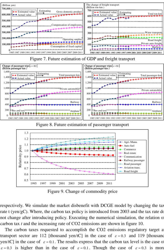
The simulating results of future are shown in figure from 7 to 10 without introducing the automobile related carbon tax, in the other words business as usual (BAU) case. As for the results on passenger trips, the estimated dynamic path of passenger-km is indicated by dividing the case into ε =0.3 and ε =0.1. Seeing this results carefully, it becomes known that automobile passenger-km in the case of ε=0.3 is estimated upper level than in the case of ε=0.1. The reason leading such results can be understood from figure 11, in which the fact declining the automobile fuel price relatively toward the future is expressed. The difference of estimated automobile passenger-km generated the

(16)

Table 4. Parameters of product function

Labor Capital

Agriculture/Manufacture 335.99 0.7448 0.2552 0.3402

Gasoline automobile industry 627.54 0.8171 0.1829 0.1787

Diesel automobile industry 627.54 0.8171 0.1829 0.1787

CEV industry 627.54 0.8171 0.1829 0.1787

Gasoline product industry 44.10 0.5274 0.4726 0.5156

Light-oil product industry 44.10 0.5274 0.4726 0.5156

Electric/gas/water 61.56 0.5616 0.4384 0.4457 Commerce 618.43 0.8154 0.1846 0.6681 Finance/insurance 224.46 0.6997 0.3003 0.6118 Real estate 0.35 0.0811 0.9189 0.8030 Railway passenter 487.29 0.7874 0.2126 0.3756 Road passenger 2007.02 0.9683 0.0317 0.7346

Private automobile passenger 0.00 0.0000 0.0000 0.0000

Aviation transport 2381.18 0.9987 0.0013 0.3151

Railway freight 1996.07 0.9674 0.0326 0.4140

Road freight 1658.06 0.9404 0.0596 0.6429

Private automobile Freight 0.00 0.0000 0.0000 0.0000

Water transport 840.15 0.8523 0.1477 0.3569

Communication 407.79 0.7668 0.2332 0.5867

Official 2364.47 0.9969 0.0031 0.6609

Service 588.82 0.8096 0.1904 0.5592

Scale parameter Share parmaeter Pruduct

capacity ratio η L α αK 0 a

Table 5. Parameters of utility, investment and government consumption functions

First stage Investment Government

elasticity of substitution 1.113 Agriculture/Manufacture 0.815 0.010

Share parameter(Present goods) 0.787 Gasoline automobile industry 0.033 0.000

(Savings) 0.213 Diesel automobile industry 0.006 0.000

Second stage CEV industry 0.000 0.000

elasticity of substitution 0.8 Gasoline product industry 0.000 0.000

Share parameter(Composite goods) 0.617 Light-oil product industry 0.000 0.000

(Leisure) 0.252 Electric/gas/water 0.000 0.024

(Total passenger tirp) 0.130 Commerce 0.075 0.000

Third stage Finance/insurance 0.000 0.000

Share parameter(Agri./Manu.) 0.144 Real estate 0.000 0.000

(Electric/gas/water) 0.015 Railway passenter 0.000 0.000

(Commerce) 0.198 Road passenger 0.000 0.000

(Finance/insurance) 0.015 Private automobile passenger 0.000 0.000

(Real estate) 0.134 Aviation transport 0.000 0.000

(Total freight transport) 0.021 Railway freight 0.000 0.000

(Communication) 0.009 Road freight 0.005 0.000

(Official) 0.102 Private automobile Freight 0.000 0.000

(Service) 0.361 Water transport 0.000 0.000

Fourth stage Communication 0.000 0.000

elasticity of substitution 0.8 Official 0.000 0.361

Share parameter(Railway freight) 0.0053 Service 0.066 0.605

(Road transport) 0.7683 Endowment of time 291,807[Million hour]

(Private auto freight) 0.0000 Capital Stock in 1995 932,235,000[Billion yen]

(Water transport) 0.2265 Capital consumption ratio 0.09734

H β H β − 1 1 σ 2 σ X γ S γ P γ 1 ς 2 ς 3 ς 4 ς 5 ς F ς 6 ς 7 ς 8 ς T χ R χ A χ S χ F σ j ξ ζj Ω 1995 S K K δ

Table 6. Parameters of passenger transport service consuming model

The case of The case of

Purchasing Fuel choice Modal Choice Purchasing Fuel choice Modal Choice Logit parameter -0.00995 -0.00995 -0.550 -0.00995 -0.00995 -0.190 Constant term 0.298 -3.558 1.627 0.298 -3.558 -0.734 B θ _θS _θM _θB _θS _θM 3 . 0 = ε ε=0.1

one of CO2 emissions gotten in the both case of ε=0.3and ε=0.1. The estimated

increasing rate of CO2 emissions in 2010 comparing with 1990 is 43.0% in the case of

3 . 0

=

ε , and is 39.0% in the case of ε=0.1.

5.3Result of simulation for introducing the carbon tax

The carbon tax levied on CO2 emissions is indicated as t [yen/gC]. Using the coefficients of CO2 emissions that of gasoline is 643 [gC/l] and of light-oil is 721 [gC/l], the imposed amounts of carbon tax are obtained as 643t [yen] and 721t [yen],

(17)

Estimating _{Gross domestic product}

Compensation of employees

Operating surplus Consumption of fixed capital Estimated value Actual value 1985 1987 1989 1991 1993 1995 1997 1999 2001 2003 2005 2007 2009 2011 0 100,000 200,000 300,000 400,000 500,000 600,000 700,000 (Billion yen) 0 100 200 300 400 500 600 700 1985 1987 1989 1991 1993 1995 1997 1999 2001 2003 20052007 2009 2011

The change of freight transport (Billion ton-km )

Total ton-km

Road freight Water transport Estimating

Private auto freight Railway Estimated value

Actual value

Operating surplus Consumption of fixed capital Estimated value Actual value 1985 1987 1989 1991 1993 1995 1997 1999 2001 2003 2005 2007 2009 2011 0 100,000 200,000 300,000 400,000 500,000 600,000 700,000 (Billion yen)

Operating surplus Consumption of fixed capital Estimated value Actual value 1985 1987 1989 1991 1993 1995 1997 1999 2001 2003 2005 2007 2009 2011 0 100,000 200,000 300,000 400,000 500,000 600,000 700,000 0 100,000 200,000 300,000 400,000 500,000 600,000 700,000 (Billion yen) 0 100 200 300 400 500 600 700 1985 1987 1989 1991 1993 1995 1997 1999 2001 2003 20052007 2009 2011

Total ton-km

Private auto freight Railway Estimated value Actual value 0 100 200 300 400 500 600 700 0 100 200 300 400 500 600 700 1985 1987 1989 1991 1993 1995 1997 1999 2001 2003 20052007 2009 2011 1985 1987 1989 1991 1993 1995 1997 1999 2001 2003 20052007 2009 2011

Total ton-km

Private auto freight Railway Estimated value

Actual value Estimated value Actual value

Figure 7. Future estimation of GDP and freight transport

0 200 400 600 800 1,000 1,200 1,400 1,600 1985 1987 1989 1991 1993 1995 1997 1999 2001 2003 2005 2007 2009 2011 Total passenger-km Estimating Estimated value Actual value Private automobile Railway Airplane Bus and taxi

Change of passenger trips (Billion passenger-km ) [ 03] . ε= 0 200 400 600 800 1,000 1,200 1,400 1,600 1985 1987 1989 1991 1993 1995 1997 1999 2001 2003 2005 2007 2009 2011 Total passenger-km Estimating Estimated value Actual value Private automobile Railway Airplane Bus and taxi

Change of passenger trips (Billion passenger-km ) [ 03] . ε= 0 200 400 600 800 1,000 1,200 1,400 1,600 1985 1987 1989 1991 1993 1995 1997 1999 2001 2003 2005 2007 2009 2011 Total passenger-km Estimating Estimated value Actual value Estimated value Actual value Private automobile Railway Airplane Bus and taxi

Change of passenger trips (Billion passenger-km ) [ 03]

.

ε=

Change of passenger trips (Billion passenger-km ) [ 01] . ε= 0 200 400 600 800 1,000 1,200 1,400 1,600 1985 1987 1989 1991 1993 1995 1997 1999 2001 2003 2005 2007 2009 2011 Total passenger-km Estimating Estimated value Actual value Estimated value Actual value Private automobile Railway Airplane Bus and taxi

.

ε=

.

ε=

Figure 8. Future estimation of passenger transport

0.5 0.6 0.7 0.8 0.9 1.0 1.1 1.2 1.3 1995 1997 1999 2001 2003 2005 2007 2009 2011 Agri./Manu. Auto fuel Commerce Real estate Communication Railway passenger Road passenger Aviation trans. Road freight Re la ti vi ty pr ic e 0.5 0.6 0.7 0.8 0.9 1.0 1.1 1.2 1.3 1995 1997 1999 2001 2003 2005 2007 2009 2011 Agri./Manu. Auto fuel Commerce Real estate Communication Railway passenger Road passenger Aviation trans. Road freight Agri./Manu. Auto fuel Commerce Real estate Communication Railway passenger Road passenger Aviation trans. Road freight Re la ti vi ty pr ic e

Figure 9. Change of commodity price

respectively. We simulate the market disbenefit with DCGE model by changing the tax rate t (yen/gC). Where, the carbon tax policy is introduced from 2003 and the tax rate do not change after introducing policy. Executing the numerical simulation, the relation of carbon tax t and the increasing rate of CO2 emissions are shown in figure 10.

The carbon taxes requested to accomplish the CO2 emissions regulatory target at transport sector are 112 [thousand yen/tC] in the case of ε=0.3 and 119 [thousand yen/tC] in the case of ε=0.1. The results express that the carbon tax level is the case of

3 . 0

=

ε is higher than in the case of ε=0.1. Though the case of ε=0.3 is more

sensitive for introducing the policy, the reason led such results is considered that the CO2 emissions of BAU case is more increasing in the case of ε=0.3 than ε=0.1. In figure 10, the relation between the carbon tax and automobile fuel price of gasoline

(18)

0% 10% 20% 30% 40% 50% 60% 70% 80% 20 40 60 80 100 120

Carbon tax [thousand yen/tC] CO2increasing rate in 2010

comparing with 1990

Price elasticity : 0.3 Price elasticity : 0.1

Regulatory target at transport sector [17%]

112 119 Existing state 0 50 100 150 200 250 0 20 40 60 80 100 120

Carbon tax [thousand yen/tC] Fuel price [yen/l]

112 119 Gasoline Light-oil 113.2 119.2 169.8 197.3 0% 10% 20% 30% 40% 50% 60% 70% 80% 20 40 60 80 100 120

Carbon tax [thousand yen/tC] CO2increasing rate in 2010

comparing with 1990

Price elasticity : 0.3 Price elasticity : 0.1

112 119 Existing state 0 0% 10% 20% 30% 40% 50% 60% 70% 80% 0% 10% 20% 30% 40% 50% 60% 70% 80% 20 40 60 80 100 120 20 40 60 80 100 120

Carbon tax [thousand yen/tC] CO2increasing rate in 2010 comparing with 1990 Price elasticity : 0.3 Price elasticity : 0.1 Price elasticity : 0.3 Price elasticity : 0.1

112 119 Existing state 0 50 100 150 200 250 0 20 40 60 80 100 120

112 119 Gasoline Light-oil 113.2 119.2 169.8 197.3 50 100 150 200 250 0 20 40 60 80 100 120

112 119 Gasoline Light-oil Gasoline Light-oil 113.2 119.2 169.8 197.3

Figure 10. Carbon tax and CO2 increasing rate, and fuel price

and light-oil is also drawn. Seeing this graph, it is indicated that rising rate of light-oil price for increasing carbon tax is higher than the one of gasoline price. From this figure, the fuel prices when introducing the carbon tax policy to accomplish the regulatory target, become clear that the gasoline and light-oil prices are 113.2(yen/l) and 169.8(yen/l) respectively in the case of ε=0.3 , and those are 119.2(yen/l) and 197.3(yen/l) respectively in the case of ε=0.1.

Next, the measured results of market disbenefit are shown in figure 11. They are 1,810(Billion yen) in the case of ε=0.3 and 2,490(Billion yen) in the case of ε =0.1. Here, in the figure 11, the point that the market disbenefit becomes zero implies the role as the carbon tax of the fuel tax levied at present. Hence it is calculated that the increasing rates of carbon tax to accomplish the regulatory target are 83.1% in the case of ε=0.3, and 95.1% in the case of ε=0.1.

-1,000 -500 0 500 1,000 1,500 2,000 2,500 3,000 M ar k et di sb e n e fi t [B illi o n y e n ] 20 40 60 80 100 120

Carbon tax [thousand yen/tC]

112 119 2,490 1,810 Price elasticity : 0.3 Price elasticity : 0.1 Existing state -1,000 -500 0 500 1,000 1,500 2,000 2,500 3,000 -1,000 -500 0 500 1,000 1,500 2,000 2,500 3,000 M ar k et di sb e n e fi t [B illi o n y e n ] 20 40 60 80 100 120 20 40 60 80 100 120

Carbon tax [thousand yen/tC]

112 119 2,490 1,810 Price elasticity : 0.3 Price elasticity : 0.1 Price elasticity : 0.3 Price elasticity : 0.1 Existing state

Figure 11. Carbon tax and market disbenefit

5.4Result of simulation for the subsidy to the clean energy vehicle

As for the subsidy to the clean energy vehicle, we simulate the change of increasing rate of CO2 emissions and the market disbenefit with introducing the subsidy policy and obtain the result shown in figure 12. Where, the price elasticity is set ε=0.1 and carbon tax level is done t = 112[thousand yen/tC].

(19)

0% 2% 4% 6% 8% 10% 12% 14%

Market disbenefit

CO2 increasing rate (from 1990) Without the subsidy for CEV

The subsidy rate for Clean Energy Vehicle 500 1,000 1,500 2,000 2,500 20% 22% 6% 8% 10% 12% 14% 16% 18% 24% 1.83 M arket d is b e n e fit ( B il lio n y e n) C O 2 in c reas ing r a te in 2010 c o m p ar in g w it h 1 990 17.0% 0% 2% 4% 6% 8% 10% 12% 14% Market disbenefit

CO2 increasing rate (from 1990) Without the subsidy for CEV Market disbenefit

CO2 increasing rate (from 1990) Without the subsidy for CEV

The subsidy rate for Clean Energy Vehicle 500 1,000 1,500 2,000 2,500 500 1,000 1,500 2,000 2,500 20% 22% 6% 8% 10% 12% 14% 16% 18% 24% 1.83 M arket d is b e n e fit ( B il lio n y e n) C O 2 in c reas ing r a te in 2010 c o m p ar in g w it h 1 990 17.0%

Figure 12. Subsidy rate for CEV and CO2 increasing rate or market disbenefit less for raising the subsidy rate, and the market disbenefit has been generating more. As for the impact that the subsidy gives to market disbenefit, it is thought the effect by being declined the price of clean energy vehicle and negative effect by being decreased the carbon tax revenue through the government service. From the result, we are known that the reducing the CO2 emissions can be done by 6.4% of subsidy rate without generating more market disbenefit.

6. Conclusion

In this paper, the impacts with introducing the automobile related carbon tax have been evaluated by using the dynamic computable general equilibrium (DCGE) model. Here, setting the difference price elasticity in the fuel demand, the reducing volume of CO2 emissions and market disbenefit have been computed for each case. Those results are concluded as below.

i) The case of price elasticity ε=0.3: The carbon tax requested to accomplish the CO2 emissions regulatory target at transport sector (to control CO2 emissions by 17% increasing in 2010 comparing with 1990) is 112[thousand yen/tC]. However, in which the present fuel tax is included, hence its carbon tax level is equivalent to the raising tax rate 83.1% comparing with present situation. With introducing this carbon tax policy, the market disbenefit is generated 1,810[Billion yen] and the GDP is declined by 0.5%.

ii) The case of price elasticity ε=0.1: The requested carbon tax of this case is 119[thousand yen/tC], and the raising tax rate is 95.1%. With introducing this policy, the market disbenefit is 2,490[Billion yen] and the GDP is declined by 0.56%.

From these results, it has been known that the difference of fuel price elasticity does not give so serious impact to the reduction of CO2 emissions. The reason is thought that the effects decreasing CO2 emissions with policy is possible to cancel out by changing the CO2 emissions in BAU case, if the price elasticity is set to difference case.

However, in this study, we could not analyze the impacts by changing the fuel price elasticity of transport industry sectors. And it is remained as future tasks that are the reconsideration of myopic expectation or the analysis introducing the carbon tax for industrial sector except automobile sector.

(20)

Acknowledgement

This study is financially supported by the Scientific Grant-in-Aid of the Ministry of Education, the Government of Japan.

References

Ballard, C.L. and Medema, S.G. (1993): “The marginal efficiency effects of taxes and subsidies in the presence of externalities” Journal of Public Economics52, 199-216.

Bergman, L. (1991): “General equilibrium effects of environmental policy: a CGE-modeling approach” Environmental and Resource Economics1, 43-61.

Borger, B.D. and Swysen, D. (1998): “Optimal Pricing and Regulation of Transport Externalities: A Welfare Comparison of Some Policy Alternatives” in Roson, R. and Small, K.A. (eds), Environmental and Transport in Economic Modelling, Kluwer Academic Publishers, Chapter 6, 118-151.

Goulder, L.H., I.W.H. Parry, R.C. Williams III. And D. Burtraw (1999): “The cost-effectiveness of alternative instruments for environmental protection in a second-best setting” Journal

of Public Economics72, 329-360.

Jorgenson, D.W. and Wilcoxen, P.J. (1990): “Intertemporal general equilibrium modeling of U.S. environmental regulation” Journal of Policy Modeling12-4, 715-744.

McFadden, D. (1981): “Econometric models of probabilistic choice, structural analysis of discrete data with econometric applications” in C.F. Manski and D. McFadden (eds), MIT press, Chapter 5, 198-272.

Mayeres, I. (2000): “The efficiency effects of transport policies in the presence of externalities and distortionary Taxes” Journal of Transport Economics and Policy34-2, 233-360. Miyagi, T. (1986): “On the formulation of a stochastic user equilibrium model consistent with

the random utility theory: a conjugate dual approach” Selected Proceeding of WCTR ’86, 1619-1635.

Rana, A. (2003): “Evaluation of a renewable energy scenario in India for economic and CO2 mitigation effects” journal of the applied regional science conference (RURDS) 15-1, 45-54.

Roson, R. (2003): “Climate change policies and tax recycling schemes: Simulations with a dynamic general equilibrium model of the Italian economy” journal of the applied regional science conference (RURDS) 15-1, 26-44.

Shoven, J.B. and Whalley, J. (1984): “Applied general equilibrium models of taxation and international trade: an introduction and survey” Journal of Economic Literature 22, 1007-1051.

Shoven, J.B. and Whalley, J. (1992): Applying general equilibrium, Cambridge University Press, Cambridge.