Machine learning analytics for predictive breeding

2020

Machine learning analytics for predictive breeding

Machine learning analytics for predictive breeding

Iowa State University

Follow this and additional works at: https://lib.dr.iastate.edu/etd

Recommended Citation Recommended Citation

Xu, Zhanyou, "Machine learning analytics for predictive breeding" (2020). Graduate Theses and Dissertations. 18248.

https://lib.dr.iastate.edu/etd/18248

This Dissertation is brought to you for free and open access by the Iowa State University Capstones, Theses and Dissertations at Iowa State University Digital Repository. It has been accepted for inclusion in Graduate Theses and Dissertations by an authorized administrator of Iowa State University Digital Repository. For more information, please contact [email protected].

by Zhanyou Xu

A dissertation submitted to the graduate faculty in partial fulfillment of the requirements for the degree of

DOCTOR OF PHILOSOPHY

Major: Bioinformatics and Computational Biology

Program of Study Committee: William D. Beavis, Co-major Professor

Steven Cannon, Co-major Professor Silvia Cianzio

Jode Edwards Julie A. Dickerson

The student author, whose presentation of the scholarship herein was approved by the program of study committee, is solely responsible for the content of this dissertation. The Graduate College will ensure this dissertation is globally accessible and will not permit alterations after a

degree is conferred.

Iowa State University Ames, Iowa

2020

TABLE OF CONTENTS

Page

ABSTRACT ...v

CHAPTER 1. GENERAL INTRODUCTION ...1

Dissertation organization ... 4

CHAPTER 2. LITERATURE REVIEW ...6

Part 1: An abiotic trait: Soybean iron deficiency chlorosis (IDC) ... 6

Part 2: A biotic trait: Soybean sudden death syndrome (SDS) ... 19

Interaction network of genes associated with traits of interest ... 23

Part 3: Spatial data analyses for adjusting phenotypic data ... 24

What is spatial data analysis? ... 25

Spatial pattern recognition and phenotypic adjustment to improve prediction accuracy ... 25

Spatial adjustment for phenotypic data ... 27

Spatial autoregressive regression (SAR) models ... 28

Model comparison and Lagrange Multiplier Test (LMT) ... 30

Application of SAR models ... 31

Part 4: Genomic prediction methods and machine learning algorithms ... 39

CHAPTER 3. GEOSPATIAL STATISTICS FOR SOYBEAN IRON DEFICIENCY CHLOROSIS ...60

Abstract ... 60

Introduction ... 61

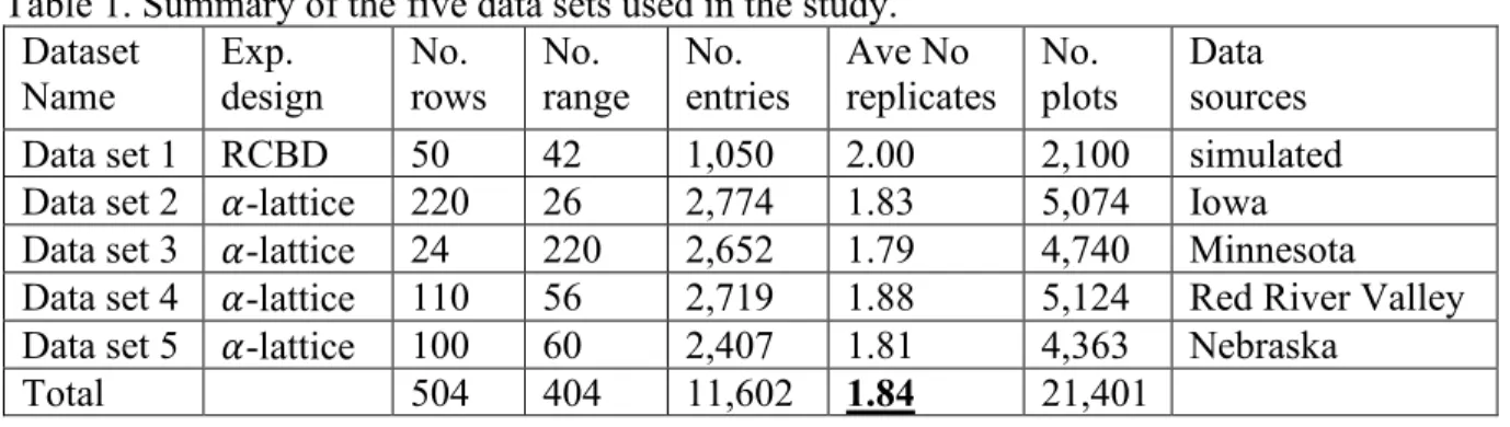
Data and methods ... 68

Data ... 68

Analytic methods ... 72

Performance metrics to compare the models ... 79

Heatmap and Lagrange Multiplier Test... 81

Relative efficiency (RE) ... 82

Results and discussion ... 82

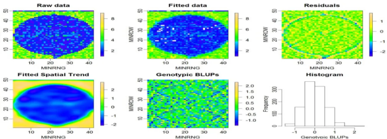
Results from the P-spline model SpATS ... 82

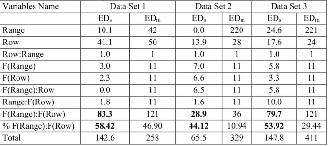
Spatial effective dimension (EDs) and the importance of surface trend by f(row):f(range) ... 85

Variance components analysis and importance of surface trend by f(row):f(range) ... 86

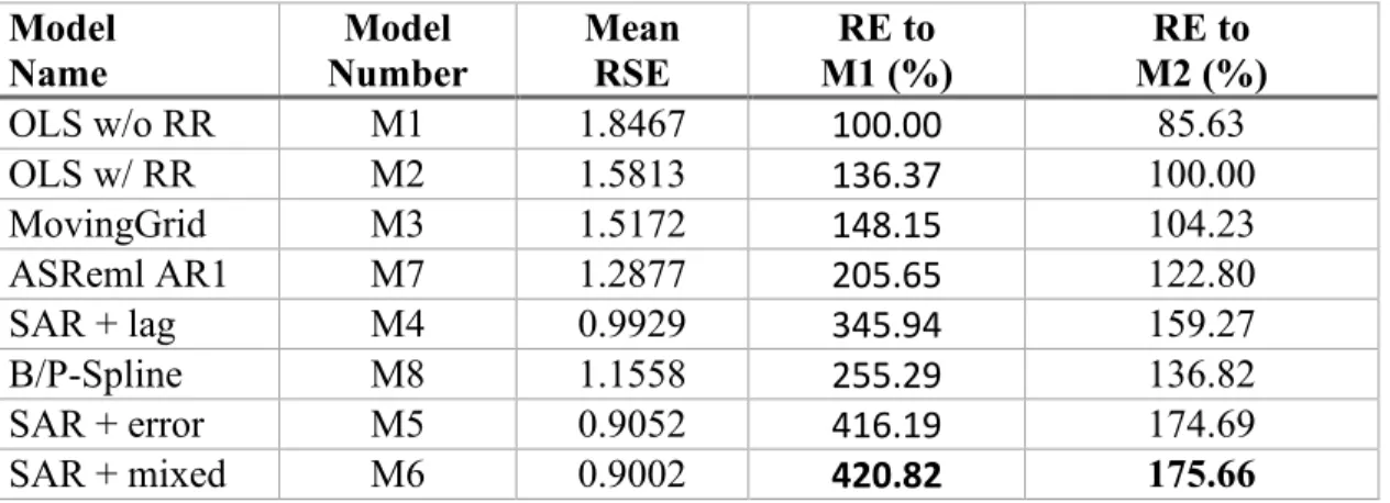
Comparison metrics among the eight models ... 88

Relative efficiency (RE) of the spatial autoregressive (SAR) analyses ... 96

Lagrange multiplier test (LMT) ... 97

Statistical experiment design for spatial analysis versus breeding practice ... 98

IDC hill plot size and spatial variation ... 99

The tensor product penalized splines may work better for continuous data type than for ordinal data type ... 101

Conclusion ... 101

Supplemental data available ... 102

Acknowledgments ... 102

References ... 102

CHAPTER 4. ALGORITHMIC MODELING VS. DATA MODELING: WILL THE ALGORITHMIC OUTPERFORMS DATA MODELING FOR IRON DEFICIENCY CHLOROSIS RESISTANCE? ...109

Abstract ... 109

Introduction ... 110

Data and Methods ... 117

Data ... 117

Analytic methods ... 117

Measurement metrics for prediction accuracy ... 118

Results and discussion ... 120

IDC overall prediction accuracy from data modeling, rrBLUP, and logistic regression . 120 IDC prediction results from algorithmic modeling, support vector machine (SVM) ... 121

IDC prediction results from algorithmic modeling, Naïve Bayes (NB)... 124

IDC prediction results from algorithmic modeling, K-nearest neighbor (KNN) ... 125

IDC prediction results from algorithmic modeling, artificial neural network (ANN) ... 126

IDC prediction results from algorithmic modeling, Gradient Boosting Machine (GBM) ... 127

IDC prediction results from algorithmic modeling, random Forest (RF) ... 129

Summary from algorithmic modeling: SVM, NB, KNN, ANN, GBM, and RF ... 130

Summary of the model performance measured by AUC from both algorithmic and data models ... 132

Models separation by principal component analysis (PCA) ... 134

Algorithmic vs. data modeling: Multiple comparisons and groups ... 135

Conclusion ... 136

Conflict of interest ... 136

Supplemental data available ... 137

Acknowledgments ... 137

References ... 137

CHAPTER 5. MACHINE LEARNING FOR SOYBEAN SDS ANALYSIS ...157

Abstract ... 157

Introduction ... 158

Materials and analytic method ... 160

Materials ... 160

Analytic Method ... 161

Model and parameter selection for Random Forest analysis ... 161

Model and parameter selection for stepwise regression analysis ... 162

Model and parameter selection for GWAS analysis by Tassel ... 162

Results and discussions ... 163

Predictive variable selection results from random forest analysis ... 163

Predictive variable selection results from stepwise regression by JMP 12 Pro ... 164

Predictive variable selection results from GWAS by Tassel 5 ... 165 Comparison of marker selection result among the three methods: random forest,

stepwise regression, and GWAS ... 166

Results of the selection of the overlapped SNPs from the three analyses: random forest, stepwise regression, and GWAS ... 168

SNP-SNP interaction network ... 169

Conclusions ... 170

Conflict of interest ... 170

Supplemental data available ... 170

Acknowledgments ... 171

References ... 171

CHAPTER 6. DISTRIBUTION AND EVOLUTION OF COTTON FIBER DEVELOPMENT GENES IN THE FIBRELESS G. RAIMONDII GENOME ...190

Abstract ... 190

Introduction ... 191

Materials and Methods ... 194

Sources of the cotton Unigenes used in this study ... 194

Mapping of cotton EST Unigenes to chromosomes of the tetraploid (G. hirsutum) At and Dt subgenomes, and the diploid (G. raimondii) D genome ... 195

Results ... 196

Distribution of fiber initiation Unigenes among chromosomes of the tetraploid At subgenome and the diploid D genome ... 196

Distribution of fiber initiation Unigenes among chromosomes of the tetraploid Dt subgenome and the diploid D genome ... 198

Distribution of fiber elongation Unigenes among chromosomes of the tetraploid At subgenome and the diploid D genome ... 199

Distribution of fiber elongation Unigenes among chromosomes of the tetraploid Dt subgenome and the diploid D genome ... 201

Distribution of fiber second cell wall deposition (SCWD) Unigenes among chromosomes of the diploid D genome and the tetraploid At and Dt subgenomes ... 201

Overall summary of the distribution of fiber initiation, fiber elongation, and SCWD Unigenes in recombination hotspot regions between the tetraploid At and Dt subgenomes vs. the diploid D genome ... 203

Chromosomal distribution of the At- or Dt-specific fiber initiation Unigenes ... 204

Chromosomal distribution of the At- or Dt-specific fiber elongation Unigenes ... 205

Visualization of the fiber Unigenes among At subgenome, Dt subgenome, and diploid D genomes... 207

Discussion ... 208

Distribution of the genetically mapped sequences in the tetraploid cotton At and Dt subgenomes ... 208

Distribution of fiber development Unigenes in recombination hotspot regions of the tetraploid At and Dt subgenomes, and the diploid D genome... 209

Implications of this study in future applications ... 210

Conclusions ... 211

Acknowledgment ... 211

References ... 212

ABSTRACT

Prediction accuracies of genomic selection methods are affected by the quality of the phenotypic and genotypic data and by the use of appropriate analytic models in the training sets. This research focuses on the impact of data quality for ordinal traits. Ordinal scores of traits are typical for various types of stress tolerance and resistance. Established spatial models developed for continuous quantitative traits were unknown whether they can effectively adjust the spatial autocorrelation for ordinal traits with sharp transitions patterns among groups of plots in experimental field trials. The effectiveness of the spatial adjustments was systematically

compared with eight different spatial models using soybean iron deficiency chlorosis (IDC) as an example. After incorporation of the spatial pattern recognition to provide adjusted ordinal data, a comparison of prediction accuracies between algorithmic modeling and data modeling

approaches were systematically conducted. The results revealed that genomic prediction accuracies could be dramatically improved by both machine learning models and geospatial spatial analyses. Overall, algorithmic modeling outperforms data modeling methods for the soybean IDC ordinal data type. Further, machine learning algorithms provide higher prediction accuracy than traditional statistical data models in terms of sensitivity, specificity, and overall accuracy.

CHAPTER 1. GENERAL INTRODUCTION

Genomic prediction is an advanced form of marker-assisted selection in which genetic markers covering the whole genome are used so that all genes and QTLs associated with traits of interest are in linkage disequilibrium with the markers. Genomic prediction includes two steps: Step I is to train the prediction model using lines with both genotypic and phenotypic data as training sets. Step II is to predict breeding values using genotypic information of the

un-phenotyped lines, the testing sets, with the trained model and estimated parameters from step I. Genomic prediction is becoming a widely adopted tool for breeding. It makes use of historical genotypic and phenotypic information to predict genotyped but not phenotyped lines for selection decisions. The advantage of genomic prediction is that the prediction accuracy will be improved with high quality phenotypic and genotypic data accumulated across years in the training sets. Accuracies of genomic prediction are affected by the quality of genotypic and phenotypic data and by an appropriate statistical model. These three components play different roles in their effect on prediction accuracy. Among them, phenotypic data quality is the most important component but most difficult to control because of both unpredictable weather patterns from year to year and genotype by environment interactions from testing locations to locations. Of them, spatial variability in the field caused by soil property, local weather conditions, and experimental activity (such as the movements of machines during plowing, tilling, and other procedures.) is the major factor that can decrease prediction accuracies. Hence, there is a need for spatial analysis of the phenotypic data before combining phenotypic data from multi-environment trials within a year and across years. A proper phenotypic spatial analysis is a crucial prerequisite for accurate calibration of genomic prediction procedures (BERNAL-VASQUEZ

Spatial variation analysis has experienced remarkable growth in recent years in terms of theory, methods, and applications in econometrics and geo-statistics. Many models to account for the spatial variation have been developed and successfully applied to increase phenotypic data quality (ANSELIN 1988a; ANSELIN AND FLORAX 1995; ANSELIN et al. 1995; ANSELIN et al.

1996; ANSELIN 2003; ANSELIN et al. 2004; ANSELIN et al. 2010; TECHNOW 2015b). In wheat

breeding, phenotypic data quality was improved by a mixed spatial model using moving means as a covariate; subsequently, genomic prediction accuracy was increased with the spatial adjustment. In rye, a model with column and row effects generated the highest prediction accuracy of all the tested spatial models (BERNAL-VASQUEZ et al. 2014). To my knowledge,

spatial variation analysis in breeding has been applied only to adjust continuous variables, such as grain yield, plant height, flowering time, thousand kernels weight, etc. I am unaware of any published reports on the application of spatial analyses to ordinal variables, such as scores for biotic and abiotic stress traits. For example, Sudden Death Syndrome and Iron Deficiency Chlorosis when scores are recorded by experts on a scale of 1 to 9, where a score of 1 represents the most resistant and 9 represents the most susceptible.

An analytical model is the second most important factor that affects genomic prediction accuracy. There are two major categories of analytical models used with training data sets (BREIMAN 2001b). One assumes that the data are generated by a pre-defined distribution-based

stochastic data model, such as normal/ Gaussian, Poisson, binomial, logistic, exponential, etc. (BALDI AND MOORE 2012; MOORE et al. 2012). These models are referred to as data models. The

other uses algorithmic approaches and treats the relation between phenotypes and genotypes as a black box with unknown distributions. This second group of analytic approaches are referred to as algorithm models and include machine learning techniques such as support vector machine

(SVM), random forest (RF), artificial neural network (ANN), Naïve Bayes Classifier (NBC), k-nearest neighbor (KNN) and so on (GUTIERREZ AND SAFARI BOOKS ONLINE (FIRM)). Logistic

regression and ridge-regression BLUP (rrBLUP) belong to data models because the prerequisite assumptions for these models are that the data follow s-shape and bell-shaped distributions, respectively (MOORE et al. 2012). In contrast, majority of the machine learning and deep

learning algorithms (SVM, ANN, KNN, RF, GBM) belong to algorithm models because no pre-defined distribution assumptions are needed (CAELLI AND BISCHOF 1996; LAVINE et al. 2004;

MCDERMOTT et al. 2013; KRUPPA et al. 2014; BEHMANN et al. 2015). In the past decades,

comparisons between data models and algorithm models have been conducted revealing that sometimes data models produce more accurate predictions than algorithm models, sometimes they are less accurate (BREIMAN 2001b; COX et al. 2001; IOANNIDIS 2005). These results suggest

that estimates of accuracy depend on whether the data meet the prerequisite statistical distribution and model assumptions (HOWARD et al. 2014). Complex quantitative traits,

including biotic traits, such as soybean sudden syndrome (SDS), flowering and relative maturity (RM), abiotic trait, such as iron deficiency chlorosis (IDC), will be used in this study as

examples to compare the prediction accuracy between the data models and the algorithm models. The objectives of this dissertation included:

1) To assess the effectiveness of spatial models to correct spatial patterns in ordinal data from field plots. Because none of the existing data model methods were capable of removing spatial patterns exhibiting sharp phase changes in ordinal data, a unique algorithmic model was developed for these types of patterns.

2) To compare the impacts of spatial adjustments to ordinal phenotypes on genomic prediction accuracies.

3) To compare algorithmic and data models based on prediction accuracies of spatially adjusted ordinal data.

4) To identify the network of genes and QTLs that may control SDS using machine learning algorithms, especially by multivariate adaptive regression splines (MARS), which can detect a high degree of interactions.

5)

Dissertation organization

This dissertation is organized into six chapters and one appendix of word file generated from R markdown scripts, which contains all the R codes and results.

Chapter 1 provides a general introduction and organization of this dissertation

Chapter 2 provides a literature review, including four parts: 1): An abiotic trait: Soybean iron deficiency chlorosis (IDC); 2): A biotic trait: Soybean sudden death syndrome (SDS); 3): Historical and current research on spatial data analysis; 4): Genomic selection and machine learning algorithms

Chapter 3 covers the comparison results of the phenotypic data adjustment from different spatial models. This chapter represents a manuscript for publication.

Chapter 4 covers comparison accuracies of predictions from data and algorithmic models, including rrBLUP, logistic regression, GBM, SVM, KNN, Naïve Bayes classification, and deep learning ANN. This chapter is being prepared as a manuscript for publication. This chapter represents a manuscript for publication.

Chapter 5 covers the results for SDS analysis to identify the interaction network of genes which may control SDS resistance pathways using machine learning algorithms. This chapter represents a manuscript for publication.

Chapter 6 is a published manuscript using bioinformatics and computational methods to study the distribution and evolution of genes in recombination hotspot regions in the cotton genome. This manuscript was developed and published using computational tools learned early in the BCB curricula at Iowa State University and is only loosely related to the theme of this dissertation.

The appendix is a word document generated from R markdown files that contain all the R codes used in this study and derived tables and figures from the R scripts.

CHAPTER 2. LITERATURE REVIEW

Part 1: An abiotic trait: Soybean iron deficiency chlorosis (IDC)

Iron is an essential micronutrient for the plant. Besides being needed in chlorophyll, Iron is also involved in the energy transfer of the plant, is part of metabolism enzymes, and is needed in the root nodule formation associated with the N-fixation. Iron deficiency chlorosis (IDC) in soybeans is caused by the inability of the plant to utilize iron in the soil. Without enough soluble iron for plants, chlorophyll production is hampered, and the plant will suffer and possibly die. IDC may occur when IDC susceptible varieties are grown on calcareous soils (NIEBUR AND FEHR

1981). IDC mainly found in the Midwest of the US, especially Iowa, Minnesota, Nebraska, and South and North Dakota (FROEHLICH AND FEHR 1981; FRANZEN AND RICHARDSON 2000).

IDC is expressed in new leaf tissue, and symptoms typically appear on younger leaves between the first and third trifoliate growth stages from vegetative V1 to V3 (LIN et al. 1998).

The typical symptom of IDC is the yellowing leaves with interveinal chlorosis, while the veins remain green (GOOS AND JOHNSON 2000). Chlorosis is the result of low chlorophyll formation

due to iron deficiency. If the adverse soil condition for IDC development is not severe and short, soybean plants may be able to absorb sufficient soluble iron and recover from the chlorosis, and yellowing symptoms cannot be recognizable by breeders. If the adverse soil condition for IDC development continues deteriorating, with severe iron deficiency, leaf edges and growing points become necrotic. With the progress of necrosis, the leaves will die and fall off the plant, and eventually, the entire plant will die. The bird view of IDC symptoms in a field in the Midwest of the US is patches of an area with yellowing plants scattered across the field.

Soybeans are the second-most-planted field crop in the United States after corn, ~ 80 million acres planted from 2010, and with a record-high 85.1 million acres planted in 2015 based

on the National Agriculture Statistics Service (NASS). More than 80% of US soybean acreage is concentrated in the upper Midwest (http://www.usda.gov/nass/pubs/todayrpt/acrg0615.pdf). A big portion of the soybean production areas in the upper Midwest is prone to IDC. Yield reduction from IDC was observed as early as in the 1960s (BURAU 1965). The first study of a

quantitative measure of yield loss regression on chlorosis score showed that the relationship between yield loss and IDC sore is linear and has a 20% yield reduction for each unit increase in chlorosis based on chlorosis scores of 1, for no yellowing symptom, to 5, for severe yellowing, leaf and plant die, (FROEHLICH et al. 1980). Based on a survey of 79 soybean producers in

Upper Midwest regions, 99% of the soybean producers indicated that IDC was a major

production issue, and 24% of their soybean crops were affected by IDC, generating an estimated 12 bu/acreyield loss per annum (HANSEN et al. 2003). Soybean iron deficiency planting acreage

is increasing from 1979 to 2012. A 160% increase in soybean production area into regions with soil pH of 7.2 or greater in the past 30 years. This increase of soybean production area into iron deficiency prone regions has led to yield losses of 340 million tons and worth an estimates $120 million dollars per year (HANSEN et al. 2004). Current IDC trends in soybean production areas

are expected to continue, thus, minimizing or eliminating yield lost due to IDC is critical. A large number of research studies have been conducted to better understand the soil and environmental properties associated with iron deficiency chlorosis in soybean (BURAU 1965;

FROEHLICH et al. 1980; TRIMBLE AND FEHR 1983; KAUR et al. 1984; HINTZ et al. 1987; CLARK et

al. 1988; LOEPPERT et al. 1988; LONGNECKER AND WELCH 1990; SINGH AND DAYAL 1992;

GONZALES et al. 1998; LUCENA 2000; HELMS et al. 2010; ALVAREZ-FERNANDEZ et al. 2011;

IDC symptoms and directly and indirectly causal factors into three aspects: 1) soil characteristics, 2) weather conditions, and 3) soybean genotype and physiology.

Several soil factors including, but not limited to, the following: soil moisture, soluble salt, calcium carbonate (CaCO3), bicarbonate (HCO3-), and nitrate (NO3-) content, and soil pH (BURAU 1965; LOEPPERT et al. 1988; MORRIS et al. 1990; FRANZEN AND RICHARDSON 2000;

BLOOM et al. 2011). While all of these soil factors have been implicated with iron deficiency

chlorosis, not all have been consistently associated with chlorosis in both field and nutrient solution experiments. The conclusion from these studies is that these soil factors determine the form of iron, soluble, or insoluble for soybean. Soils usually have a sufficient quantity of iron, but it might not be in the required soluble and ready to be absorbed by soybean plants. If the final results of iron form the combination of the soil factors is ferric hydroxide Fe (OH) 3, which is the soluble form of Fe in Fe (III), ferric. But, this soluble Fe(III) becomes insoluble with pH value from 7.2 to 8.4 and a high level of calcium carbonate (MORRIS et al. 1990).

Soil nitrate is a causative factor in iron deficiency chlorosis in soybeans (BLOOM et al.

2011). While soybean plants have the ability to fix N through root nodules, they will take up nitrate directly from the soil when it is available. When root takes up nitrate, they release bicarbonate. Overtime, bicarbonate levels can increase in soil, and the accumulated bicarbonate reduces the level of soluble iron, which eventually lead to the development of IDC symptoms. Weather also plays a role in IDC symptom development. Optional weather condition for IDC symptom development includes cool temperature and wet soils. When soils are wet, there is limited air exchange with the atmosphere, which causes a buildup of carbon dioxide in the soil. The carbon dioxide is produced by roots and soil microbes through respiration. The amount of bicarbonate in the soil is proportional to the amount of carbon dioxide, and as carbon dioxide

increases, so does bicarbonate. This increase will rapidly neutralize the acidity around the soybean root. The amount of bicarbonate in the soil has been positively correlated with IDC in soybean in the field (KAISER et al. 2014).

Based on the physiological response to Iron deficiency in the soil, plants were divided into two types: Strategy I and Strategy II plants (MARSCHNER et al. 1986). Under iron stress, Strategy I plants, through their roots, will respond to the iron deficiency through three

approaches (1) acidifying the rhizosphere through excretion of protons from H+-ATPases, (2) reducing chelated Fe3+ to Fe2+ mediated by plasma membrane ferric (chelate) reductases, and (3) transferring soluble Fe2+ across the plasma membrane and into the cytoplasm via divalent iron transporters. In contrast, Strategy II plants involve excretion of phytosiderophores that bind to the insoluble form of ferric iron (Fe3+), creating a soluble complex that Strategy II plants can uptake (MARSCHNER et al. 1986; ROMHELD AND MARSCHNER 1986). Soybean and other dicot

plants belong to Strategy I plants.

Genetic analysis and mapping of IDC QTL for marker-assisted selection (MAS) breeding have accumulated a wealth of knowledge and can be divided into three stages: bi-parental

population-based mapping, connected population mapping, or network population mapping (NPM), and genome-wide association study (GWAS).

IDC genetic inheritance of the single dominance/recessive gene model was first reported in 1943 (WEISS 1943). From the analysis of 24 bi-parental populations between and among four

IDC efficient and six inefficient lines, Weiss concluded that dominant allele control iron

efficiency and the recessive allele is conditioning iron inefficiency in iron utilization. This single gene control of IDC was confirmed and modified by Dr. Cianzio that IDC was controlled by a single major gene model but additionally observed quantitative inheritance patterns, which

indicated that IDC is also controlled by modifying genes (CIANZIO AND FEHR 1980). In contrast

to the single gene theory of IDC, analysis from different genetic populations developed from different IDC tolerant donors show that IDC is quantitatively inherited (FEHR 1982). Subsequent

studies conducted with two different mapping populations with different donors by Lin

confirmed that IDC displayed both single codominant gene and polygenic inheritance patterns in Anoka x A7 and Pride B2/1412 x A1/55 mapping populations, respectively (LIN et al. 1997; LIN

et al. 2000b). Except above intraspecific bi-parental mapping population via Glycine Max x Glycine Max, an interspecific bi-parental mapping population between Glycine Max (A86-356022) and Glycine Soja (PI468916) was used to screen for IDC QTL, and three markers were associated with IDC QTL from the mapping set, but could not be confirmed in the tester set which both mapping and tester set were from the same population (DIERS et al. 1992). In order to

determine the efficiency of SSR markers in selecting for IDC resistance in breeding populations, a superior IDC tolerance, and moderate yield potential line, A97-770012, crossed with a pioneer line, P9254, with moderate IDC resistance and superior yield potential (CHARLSON et al. 2003).

From this breeding population, three SSR markers were associated with chlorosis scores at each location, but the identities of the associated markers were different at each location. From the same team, with one more year phenotypic data and 108 SSR markers which were previously mapped and associated with 8 IDC QTLs on eight molecular linkage groups, 3 of 24

polymorphic SSR markers associated with IDC tolerance in three different locations, only one SSR marker, satt481, associated with IDC tolerance across all three environments and account for 12% of the total phenotypic variation (CHARLSON et al. 2005). Most recently, QTL mapping

for iron and zinc concentration in the seeds identified one major QTL for iron accumulation on chromosome 20, which explained 21.5% of the phenotypic variation. This QTL was in the

marker interval pa_515-1-satt239, with pa_515-1 previously associated with iron efficiency QTL (LIN et al. 1997; KING et al. 2013).

In summary, IDC is a complicated quantitative trait and controlled by both major and multiple minor genes/QTL from bi-parental mapping studies. The complex inheritance of IDC is population-dependent and influenced by a significant genotype x environment interaction

(Charlson et al. 2003; De Cianzio and Fehr 1982; Rodriguez De Cianzio and Fehr 1980; Weiss 1943).

Quantitative traits like IDC are difficult traits for breeders to improve through traditional phenotypic selection methods due to the inability of a breeder to effectively select and stack numerous favorable alleles that confer IDC tolerance. Environment-independent marker-assisted selection (MAS) has been successfully used for simple qualitative traits, but not large-scale used for quantitative traits. The first challenge of using markers to select for quantitative trait loci is the ability to identify the markers that are associated with IDC tolerance, and the marker selection works across different environments/locations and years. Due to heterogeneous soil factors and the presence of genotype x environment (G x E) interactions, it is difficult to distinguish genotypic sources of variation from the environmental components responsible for chlorosis (Froechlich and Fehr, 1981; Naeve and Rehm, 2006).

Bi-parental population-based mapping has been successfully used for mapping qualitative traits but has the following limitations: 1) usually needs a large population size, but it is difficult for soybean population development due to the difficulty of manually pollination. To effectively detect marker-trait associations in complex traits such as IDC, large population sizes (>400) are required in order to provide adequate detection power for small effects QTLs (BERNARDO 2004).

(https://soybase.org/) all have less than 150 recombinants inbreed lines (RILs) or F2/F2 lines. These smaller population sizes have limited power to detect minor effect QTL typical of a quantitative trait; 2) QTL identified from the bi-parental mapping population is population-dependent. Frequently, QTLs detected in one population are not detected in other populations, or QTLs detected in one population fail to exhibit the same or similar gene effect when validated in other genetic backgrounds; 3) small effect quantitative QTL have gene by environment effects. To overcome these drawbacks of bi-parental mapping of IDC QTL, connected population mapping using many breeding populations that shared crossing parents among these populations was proposed to map universal IDC QTLs.

Markers explaining phenotypic variation were identified in one population but were not significantly associated with IDC in another population, and QTL were mapped via a bi-parental population, but the same QTLs cannot be mapped when the QTL donor parent cross with another susceptible parent. Both cases indicated the mapped QTL are population/genetic background- dependent. In order to identify QTLs that perform stably across different genetic backgrounds, connected population, or network population mapping (NPM) was employed to discover QTLs. The two main advantages of the NPM are: 1) population size was dramatically increased

compared with single bi-parental mapping populations. For example, parent “A” crosses with Parents B, C, D, E, F, and parent B cross with Parent C, D, M, N, and Q. If each population has 100 lines, the total population size will be 1,000 lines; 2) NPM can overcome QTL population-dependent issue. For the above example, if the QTL from donor parent A works in the

background A x B, A x C, … A x F, then the identified QTL works across different populations. Otherwise, if the QTL from donor parent A works only in one of the many populations, then that population-specific QTL will not be discovered by NPM. The first research used the NPM

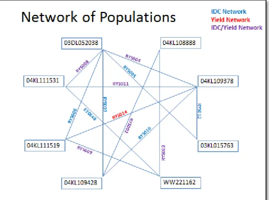
approach to map IDC was conducted by Ilene Jones (master’s degree thesis). From 8 IDC tolerant and susceptible parents, a total of 13 RIL populations were collected from Syngenta soybean IDC breeding programs (Figure 1). A total of 50 IDC QTLs were identified from the 13 disconnected bi-parental populations. In contrast, only 22 QTLs were identified in all the 8 IDC tolerant parents.

Figure 1. The network of connected mapping populations. Parent names were labeled inside rectangle boxes, and the lines show the crosses and connected network of populations. Twelve populations evaluated for iron deficiency chlorosis are depicted in blue; one population evaluated for yield is depicted in red; five populations evaluated for iron deficiency chlorosis and yield are depicted in purple.

Another project using connected network association mapping is soybean nested association mapping (NAM), which targets are to map genes/QTLs controlling soybean yield and other key traits (https://www.soybase.org/SoyNAM/). A total of 40 import soybean varieties and cultivars selected from both domestic and international exotic germplasm crossed to a common hub parent, IA3023. With 140 recombinant inbred lines (RILs) were developed from

each population, the total population size of the NAM is 5,600, which should be powerful enough to detect small effects QTLs. NAM has been successfully applied to map QTLs

controlling thousand-grain weight in barley (MAURER et al. 2016), stem rust resistance in wheat

(BAJGAIN et al. 2016), and gray leaf spot resistance in maize (BENSON et al. 2015).

Although the NPM mapping method overcomes the QTL population-dependent issue, its disadvantage is that you have to develop a large/moderate number of connected populations, and the QTLs identified limited in the small number of parents. A powerful and complementary to bi-parental and NPM mapping strategy, genome-wide association study (GWAS) that can be used to exploit historical recombination events accumulated from artificial selection (breeding) and natural selection pressure, was employed to map IDC QTLs (WANG et al. 2008; MAMIDI et

al. 2011; MAMIDI et al. 2014). From the point of analysis method for the QTL mapping view,

GWAS has applied a more advanced statistical model than that of bi-parental and NPM mapping. Both bi-parental and NPM mapping usually use simple single marker ANOVA analysis and/or composite interval mapping (CIM), which is a single-factor analysis of variance (SFA). In contrast, GWAS can use mixed linear model (MLM) except the general linear model (GLM), which the MLM treats the predictive variables as a random effect, plus including

population structure, kinship among the testing lines to reduce the number of false-positive QTLs (MAMIDI et al. 2011; VUONG et al. 2015; ZHANG et al. 2016). With the MLM analysis model,

two SSR markers (Satt14 and Satt239) were found to be associated with IDC in two independent association mapping panels, which consist of major public and private company lines.

Verification of the two markers shows that the lines with the tolerant alleles at both of these two loci have significantly lower IDC scores than lines with only one or no tolerant alleles (WANG et

GWAS with much higher density (1536 SNPs) SNP chip technology of Golden Gate and two relatively bigger association mapping panels (141 and 141 lines, respectively) was conducted, and seven genomic regions were significantly associated with IDC across two years phenotypic data. The seven loci accounted for 43.7% of the phenotypic data variation in 2005 and 47.6% in 2006 (MAMIDI et al. 2011). Most recently, GWAS was conducted to map the IDC genomic

regions with genotype-by-sequencing technology and identified seven major effect QTLs in seven chromosomes (MAMIDI et al. 2014). From this report, a total of 12 candidate genes were

associated with iron metabolism mapped near the 7 IDC QTLs, supporting the polygenic nature of soybean IDC.

The ultimate goal of QTL mapping, no matter which approach was employed, either bi-parental population-based mapping, or connected network population mapping, or GWAS, is to improve breeder’s selection accuracy via marker-assisted selection. There are several challenges that breeders face to implement the markers to stack the IDC QTLs to increase IDC breeding efficiency and accuracy:

Challenge I: no major universal IDC QTL has been discovered yet. For example, a single QTL for soybean cyst nematode (SCN) resistance from PI88788, it is a universal SCN resistant QTL and provides resistance to 99% commercial varieties (DELHEIMER et al. 2010). This QTL

provides stable resistance across global soybean germplasm, and it is a population- and

environment-independent QTL. By now, for IDC tolerance QTL discovery, the only major QTL was mapped in a population between Anoka x A7, the QTL can explain more than 70% of the phenotype variation (CIANZIO AND FEHR 1982; FEHR 1982). No further reports show that this

major IDC QTL can provide the same or similar resistance in other genetic backgrounds, or at least, the author was not successful in querying out reports about successfully transferring this

major IDC QTL to the other populations. Instead, from the same team/lab, two QTLs on MLG I/chromosome 20 and MLG N/chromosome 3 were identified in both the Pride B216 x A15 and the Anoka x A7 mapping population, respectively (LIN et al. 2000a), but, no common DNA

marker was present in both populations, and the authors concluded that the markers identified in the two mapping populations couldn’t be used in marker-assisted selection because of a general lack of common markers between the two populations (LIN et al. 2000a). The reason/mechanism

why this QTL can explain 72% phenotype variation and perform like qualitative trait but has not been widely transferred to other germplasm was being further investigated by identifying the candidate genes underlying this major QTL through molecular breeding, fine mapping, and transcriptome sequencing (PEIFFER et al. 2012). Two gene encoding transcription factors within

the major QTL were identified by transcriptome sequencing and confirmed by real-time PCR (PEIFFER et al. 2012).

One report to validate whether SSR markers previously reported associate with IDC QTLs can be used for marker assistant selection for a breeding population was conducted by Charlson (CHARLSON et al. 2005). In the report, a total of 108 SSR markers genetically linked to

8 QTLs on eight chromosomes were used to make MAS selections in a breeding population between superior and moderate IDC tolerance to test MAS selection accuracy and efficiency. Among the 108 SSR IDC markers, 24 of them are polymorphic, which the 22.22% (24/108) polymorphic rate is consistent across all soybean germplasm. The remaining 84 markers are monomorphic or homozygous in the two parental lines of the breeding population and thus not useful in screening for iron efficiency. The report did not show whether these 84 SSR markers are positively or negatively fixed in the two parental parents, even though the author wants to know and hope that they were positively fixed because the positively fixed genotype indirectly

proves the accuracy of the 84 SSR markers. Of the 24 polymorphic markers, three of them were associated with IDC resistance. However, only one marker, satt481 accounted for 12% of the total phenotypic variation, was associated with IDC tolerance across environments. Interestingly, marker Satt481 is in MLG L/chromosome 19 and is located at neither MLG N/chromosome 3 nor MLG I/chromosome 20 which are the two major QTLs reported before (RODRIGUEZ DE

CIANZIO AND FEHR 1980; LIN et al. 1997; LIN et al. 2000a). The author wants to know whether

these two QTLs were among the 84 monomorphic markers and whether they are positively or negatively fixed in the progeny from this breeding population. No matter which was the case, this example indicated that MAS might not be an ideal approach for complex quantitative trait IDC selection.

Challenge II: There is no efficient way to use MAS to stack many minor QTLs for IDC tolerance breeding by comparing the limited population size versus the number of IDC QTL to fix. By now, many IDC QTLs have been reported. From the Soybase, 39 IDC QTLs were deposited from 4 bi-parental mapping populations. From the connected network population mapping, 50 QTLs were detected via composite interval mapping (CIM) using the disconnected bi-parental model, and 22 QTLs were detected via CIM using the connected network population mapping (Thesis, Ilene Jones). From GWAS, with the strictly controlling of population structure, 42 and 88 QTLs were identified from the phenotypic data collected in 2005 and 2006,

respectively (MAMIDI et al. 2011), by the same group, 33 QTLs distributed on 10 of the 20

chromosomes were identified from the genotype-by-sequencing data (MAMIDI et al. 2014). More

recently, Transcriptome sequence profiling of soybean (Glycine max, L. Merr) near-isogenic lines Clark (PI548553, iron efficient) and IsoClark (PI547430, iron inefficient) grown under Fe-sufficient and Fe-limited conditions discovered 835 candidate genes in the Clark (PI548553)

genotype and 200 candidate genes in the IsoClark (PI547430). Of these candidate genes, and only a small portion (7~10%) of the differently expressed genes were mapped to previously identified QTL regions (O'ROURKE et al. 2009). Comparing with these large numbers of IDC

QTLs/candidate genes identified so far, Soybean is a strictly self-pollinated crop, and it is very challenging to develop large size populations to breed IDC tolerant varieties via MAS selection. For example, if an IDC population has five complimentary IDC QTLs, one mandatory herbicide marker (such as Roundup Ready RR2) and one mandatory SCN marker, then we need to select seven loci, the least F2 population size need to be (2)7_{=128 lines in order to get one plant with all} the seven loci positively fixed. This is only for the required agronomic traits, and usually,

breeders need to have 30 to 50 lines for yield variation. This leads to the population size to 128*30=3,540 lines per population, which is impossible for large-scale soybean breeding programs.

QTL-based MAS strategy has been quite useful for the manipulation of large-effect alleles with known association to a marker but not for quantitative traits that have still required extensive field testing (MOREAU et al. 2004). The methods of MAS or marker-assisted recurrent

selection assume that the user knows which alleles are favorable, and what their average effects on the phenotype are (BERNARDO AND CHARCOSSET 2006). This assumption is viable for

major-gene traits but not for quantitative traits that are influenced by many loci of small effect and the environment. In locus identification and effect estimation for such traits, much uncertainty will remain (MELCHINGER et al. 1998). To deal with quantitative traits, new statistical approaches

that could account for this uncertainty were needed to generate the best predictions possible. In conclusion, traditional marker-assisted selection has been ineffective for traits that are complex and affected by many genes and environmental factors, each with a small effect

(JANNINK et al. 2010). What is the solution for a complex trait with many minor effect alleles?

Genomic selection and machine learning for predictive breeding have arisen from the

conjunction of new high-throughput high-density chip genotyping technologies, new statistical methods, and machine learning algorithms to analyze the big data sets and provided a promising alternative to QTL-based MAS breeding.

Part 2: A biotic trait: Soybean sudden death syndrome (SDS)

Sudden death syndrome (SDS) of soybean (Glycine max (L.) Merr.), caused by the soil-borne fungal pathogen Fusarium virguliforme. It was first observed in Arkansas in 1971 and has become widespread throughout the north-central United States since then (HARTMAN et al.

2015). The fungus infects soybean root systems and produces toxins that are translocated to the leaves, resulting in premature defoliation and pod abortion (JIN et al. 1996), and eventually

leading to grain yield reduction. In recent years, SDS ranked among the top three most damaging diseases of soybean in the United States after Soybean Cyst Nematode (SCN) and Phytophthora. In the Midwestern soybean-producing area of the U.S., it is estimated that SDS has resulted in average losses valued at $190 million a year and the disease is spreading and intensifying (WRATHER AND KOENNING 2006).

SDS early symptoms of SDS are diffuse chlorotic mottling and crinkling of the leaves. Later, leaf tissue between the major veins turns yellow, then dies and turns brown. Soon after, the leaflets die and shrivel. In severe cases, the leaflets will drop off, leaving the petioles

attached. For further diagnosis from the other disease, he cortical tissue of a plant with SDS will exhibit tan to light brown streaks, whereas the cortex of a healthy plant will be white from the split lower stem.

Disease resistance breeding is believed to be the most effective approach to control SDS. Since no soybean genotypes confer complete resistance or immunity to this disease, soybean

breeders still rely on quantitative tolerance to SDS. For this purpose, many QTLs have been mapped and published via either bi-parental populations or genome-wide association studies. The first two QTLs mapped by random amplified polymorphic DNA (RPAD) marker are in chromosome 6 (linkage group LG C2) and chromosome 3 (LG N), which jointly accounted for 34% of total phenotypic variability in mean SDS disease incidence (HNETKOVSKY et al. 1996).

Two more QTLs form the same bi-parental mapping population was mapped in chromosomes 3 and 18 (LG G). Together, the four QTL accounted for about 65% of total phenotypic variability in mean disease incidence and 50% in mean disease severity (CHANG et al. 1996). Four

near-isogeneic lines (NILs) derived from a recombinant inbred line (RIL), ExF34, with heterozygous within regions of linkage group C2 and G having different resistance to SDS indicated that the QTL on linkage group G and C2 confer separate components of resistance to SDS (NJITI et al.

1998). With the application of microstate simple sequence repeat (SSR) DNA markers in QTL mapping, three more QTLs were mapped by the same group using the same mapping population (Forrest x Essex), and they were mapped in chromosome 3, 6, and 20 (LG I), interaction test of the mapped 7 QTLs indicated QTL action was additive among the loci underlying resistance to SDS (IQBAL et al. 2001). The 8th SDS QTL was mapped in C2 from variety “Douglas” with R2

0.14 (NJITI et al. 2002). From US northern varieties Minsoy and Noir1, 9th QTL was mapped in

chromosome 19 (LG L) with R2 _{0.14 (NJITI AND LIGHTFOOT 2006). By dissection resistance into} root infection and leaf scorch during soybean SDS development using the cross segregating for both SDS and Soybean cyst nematode (SCN), the 10th _{SDS QTL was discovered on chromosome} 18 underlying resistance to SDS leaf scorch with R2 _{0.13 and SCN resistance (KAZI et al. 2008).} With a much higher resolution map constructed by high-density SNP markers, seven new SDS QTLs were discovered except confirming the previous mapped 7 SDS QTLs from the bi-parental

mapping population between PI438489B’ by ‘Hamilton’(ABDELMAJID et al. 2012). These 7

“new” mapped QTLs made the total number of SDS QTLs reached to a total of 17 QTLs, 11th _to 17th_{. So far, all the 17 SDS QTLs were identified from bi-parental mapping populations.}

In order to exploit historical recombination events accumulated from artificial selection (breeding) and natural selection pressure, a powerful and complementary to bi-parental mapping strategy, genome-wide association study (GWAS), was used to map SDS QTLs. A total of 20 QTLs were discovered from two association mapping panel, and 7 of the 20 loci was overlapped to previously mapped QTL intervals, and 13 of them have not been mapped before (WEN et al.

2014). Similarly, from more recently GWAS mapping, two novel SDS QTLs were identified from chromosomes 3 and 18 (BAO et al. 2015). By integrating epistasis analysis with GWAS,

genome-wide epistasis study (GWES) used employed to discover both SDS additive and interaction effects for SDS, four new SDS QTLs and 12 SNP-SNP interaction associated with SDS resistance were identified and the epistatic effects increase SDS resistance by 5 to 20% and provide a substantial complement to additive effects. (ZHANG et al. 2015)

From above literature search and summary, 17 SDS QTLs were mapping by bi-parental mapping populations and stored in soyBase.org http://www.soybase.org), and 19 novel SDS QTLs, 13 from (WEN et al. 2014), two from (BAO et al. 2015), four from (ZHANG et al. 2015)

were mapped from GWAS, with a total of 36 unique SDS QTLs were mapped. From epistasis based GWES, 12 SNP-SNP interaction were identified.

Even though many SDS tolerant QTLs have been mapped, SDS QTL-based selection was not widely used for SDS resistant variety breeding. There may be many reasons behind it, such as 1) no SDS QTL has been proved to work across different populations or genetic backgrounds. QTLs were mapped in bi-parental populations, and these QTLs were population-specific and did

not work in other genetic backgrounds. From the testing the usefulness of 10 SDS QTLs across six populations, no single QTL works across these six populations (LUCKEW et al. 2013); 2) no

stable major SDS QTL has been identified. A total of 17 QTLs were mapped from bi-parental mapping populations, and their R2 _{values range from 2% to 63% with small population sizes} ranged from 40 to 80 per population (MEKSEM et al. 1999), but there is no major SDS QTLs as

stable and major as soybean Cyst nematode SCN resistant QTL from PI 88788 which has been provided 99% of the SCN resistance (DIERS et al. 1997); this observation was further confirmed

by GWAS study which 20 QTLs were mapped ranged from 5.3% to 11.6% with average 7.4% (WEN et al. 2014); 12 QTLs ranged from 6% to 9% with average 7.5% (ZHANG et al. 2015); 3)

impractical to stack multiple QTLs with minor QTL effects. Since SDS QTLs are quantitative, and the effects are less than 10%, breeding SDS commercial varieties need to stack multiple QTLs. Soybean is self-pollinated cleistogamous (pollinated before the flower opens) crop, with current pollination technology, it would be impractical for soybean breeders to pyramid more than 6 QTLs from different populations into a single genetic background because an unusually large population is needed (LUCKEW et al. 2013); 4) both bi-parental mapping and GWA study in

soybean mapped only the additive gene/QTL effects via single locus significant test or interval mapping, and epistasis and other gene interaction effects in soybean breeding have not to be reported by now. QTL- breeding either based on individual SNP selection or combination of SNPs as haplotype assistant selection. However, additive-effect only based selection may not be sufficient to explain the complexity of disease causality. It has been established that gene-gene/SNP-SNP interactions may have a higher impact on discovering causality of complex human disease (REAMS et al. 2011; LIN et al. 2013). There may exists two levels of interaction:

three-dimensional interaction among all these QTLs which may coordinate and cross-regulate each other in a network and function as one integrated unit. When only partial QTLs of the network were tracked and traced in MAS selection, the critical or bottleneck part of the network may be monomorphic and block the pathway; this may lead to the failure of QTL-based breeding for the complexity of the trait of SDS.

Interaction network of genes associated with traits of interest

New studies and potential solutions have been publishing to understand human diseases and may be applied to soybean SDS breeding. SNP-by-SNP interaction network study has been reported to dissect human disease. A synergetic SNP-by-SNP network of alcoholic addiction was constructed by two steps: step 1 to form the SNP-by-SNP interaction network based on prior biological knowledge and their correlation between the functional relationships of their genes; step 2 to prioritize disease-risk SNPs via their differentially inherited properties in identity by descent (IBD) (LI et al. 2011a). A weighted SNP interaction hub network was constructed for

human complex diseases and traits using whole-genome genotype data (KOGELMAN AND

KADARMIDEEN 2014). By combing two powerful machine learning methods: random forest (RF)

and multivariate adaptive regression spline (MARS), an SNP-by-SNP interaction network associated with prostate cancer was constructed (LIN et al. 2012; LIN et al. 2013). All these

reports from the study of human diseases show that SNP-by-SNP network-based prediction provides a promising opportunity to increase prediction accuracy. The goal of this study was to investigate the interaction among soybean SDS QTLs and to build both DNA and protein level interaction network of soybean SDS resistance by integrating the strengths of the four machine learning methods through 2 steps: step 1 to find the overlap SNPs from parametric-based stepwise regression with its strength in identifying a subset of most predictive variables from a large number of variables, such as high-density SNP chip data (MITCHELL et al. 2001),

genome-wide association with its strength in exploiting historical recombination events at the population level to identify more QTLs across different germplasm (TEO 2008), and non-parametric based

random forest with its strength in selecting important variables based on decision tree (CHEN et

al. 2011); step 2 to identify the interaction by MARS (FRIEDMAN AND ROOSEN 1995) with its

strength in detecting SNP-by-SNP interaction patterns (LIN et al. 2012). Here we present the first

DNA level QTL interaction network, protein by protein interaction (PPI) network for soybean SDS. The identification of these QTLs in the interaction network will increase our understanding of mechanisms underlying SDS resistance, and network-based prediction by MARS via R

package “earth” (http://www.milbo.users.sonic.net/earth/) provides novel marker selection system for breeding soybean lines with SDS resistance.

Part 3: Spatial data analyses for adjusting phenotypic data

Spatial data refers to types of data objects or elements that are present in a geographical space or horizon. Spatial data is also known as geospatial data, spatial information, or

geographic information. It is the data or information that identifies the geographic location of features and boundaries on Earth, such as natural or constructed features, oceans, and breeding testing sites, etc. Spatial data is usually stored as coordinates and topology and is data that can be mapped. Spatial data is often accessed, manipulated, or analyzed through Geographic

Information Systems (GIS).

In this dissertation, spatial data refers to any phenotypic data taken from field coordinated by either by a combination of row and column numbers, or combination of Global Positioning System (GPS) longitude and latitude coordinates, such as testing plots planted by AccuRow’s GPS-guided planter (Raven Industries Sioux Falls, South Dakota, USA).

What is spatial data analysis?

Spatial analysis is a set of techniques for analyzing spatial data. The results of spatial analysis are dependent on the locations of the objects being analyzed. Software that implements spatial analysis techniques requires access to both the locations of objects and their attributes. The objectives of spatial analysis are to determine the spatial distribution of a variable, the relationship between the spatial distribution of variables, and the association of the variables of an area. It refers to the analysis of phenomena distributed in space and having physical

dimensions (MAGUIRE et al. 2005). In GIS, there are four traditional types of spatial analysis:

spatial overlay and contiguity analysis, surface analysis, linear analysis, and raster analysis. In this dissertation, spatial analysis refers to spatial surface analysis with different models to remove spatial autocorrelation and spatial dependence, which is "everything is related to everything else, but near things are more related than distant things.” This is the well-known “The First Law of Geography” by Waldo Tobler and is the foundation of the fundamental concepts of spatial dependence and spatial autocorrelation adjustment (CHAKRABORTY 2011;

KLIPPEL et al. 2011; WESTLUND 2013). Specifically, the row and columns are used as spatial

coordinates to locate the experiment plots to analyze the distribution of the plots, autocorrelation of the neighbor plots, and patterns of the plots.

Spatial pattern recognition and phenotypic adjustment to improve prediction accuracy

Figure 2. Diagram of genomic prediction. The training materials are genotyped and phenotyped to 'train' the genomic selection (GS) prediction model. Genotyped but not phenotyped breeding lines are then fed into the model to calculate genomic estimated breeding values (GEBV) for these lines.

Consider a genomic prediction analytic flowchart, such as depicted in Figure 2. There are three essential elements that will affect the accuracy of estimated predictions used for the selection: 1) quantity and quality of genotypic data, 2) quantity and quality of phenotypic data, 3) choice of appropriate analytic models for predictions. Among the three elements, the quantity and quality of genotypic assays are the most advanced. It is possible to obtain high-quality assays, as judged by reliability and repeatability, at sufficient density throughout the genome to assure those causative alleles for all traits of interest are in linkage disequilibrium (LD) in any arbitrary sample from a population of interest.

In contrast, the quality of phenotypic data, as judged by reliability and repeatability, is not at the same level as genotypic data. This is due in part to non-genetic sources of variability that affect the phenotype. These non-genetic effects include field soil characteristics that are not constant across afield as well as weather characteristics that are not consistent in space or time. It is hoped that phenotyping costs will decrease with the emergence of low-cost image acquisition and processing through computer-aided robots and drones, but data from these technologies are still being adapted to meet the data requirements of plant breeding objectives.

Many phenotypic traits, such as soybean Iron Deficiency Chlorosis (IDC), are strongly influenced by spatial variation in soil pH, soluble iron content, moisture, as well as other unknown environmental factors. Field plot experimental designs attempt to account for non-genetic sources of variability through the use of check plots (MULLER et al. 2010), replication

and blocking. Examples of field plot designs that use these techniques include a randomized complete block (RCB) and incomplete block designs such as α-lattice and augmented designs.

of field plot heterogeneity, often patterns of spatial variability remain; especially if the

orientation of irregular spatial patterns are not consistent with block arrangements (LEISER et al.

2012).

Spatial adjustment for phenotypic data

Analyses of Variance (ANOVA) using ordinary least square (OLS) are based on three assumptions: Independence 1) model parameters are independent, 2) residual variability is identically distributed, and 3) the residual variability is are normally distributed. Residual variability from field-based phenotypic data (grain yield, biomass, biotic, abiotic scores) often shows irregular spatial patterns. These data without adjustment by spatial analysis presents a challenge to the parametric and distribution assumptions. These problems are typically seen as various representations of spatial structure ornon-independence. The spatial structure of the data can introduce spatial dependence into both the outcome, the predictors, and the model residuals. These data are correlated among neighbors, named autocorrelation, and the closer the distance between neighbors, the tighter that correlations are. Both positive and negative autocorrelations for either the dependent variable, the model predictors, or the model residuals.

Various spatial adjustment techniques have been developed and have been shown to significantly improve heritability and repeatability estimates resulting in a more effective selection of targeted traits. Based on the spatial adjustment mechanism and theory, three groups of approaches have been published:

1) Group 1: Spatial Autoregressive Regression (SAR) models including spatial lag models, spatial error models, and mixed spatial models (ANSELIN 2001; ANSELIN 2003;

DORMANN et al. 2007a)

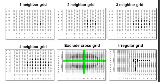
2) Group 2: Moving grid adjustment: a grid or pattern consisting of neighboring plots are predefined for each plot, the mean of the plots included in the grid is calculated and used

as a covariate to account for the spatial variation (TECHNOW 2015b). This approach has

been reported to increase genomic selection accuracy in wheat breeding (LADO et al.

2013a).

3) Group 3: Tensor product penalized spline models. These models include both bilinear polynomial and smooth splines components. The bilinear polynomial component includes three sub-variables: row spatial trend, column spatial trend, and interaction between row and columns. The smooth spline part includes five smooth additive spatial components (Rodríguez-Álvarez et al., 2017)

Spatial autoregressive regression (SAR) models

Spatial effects can be divided into two categories: spatial dependence and spatial

heterogeneity. Spatial dependence deals with autocorrelation, and spatial heterogeneity refers to structural instability, either in the form of non-constant error variances in a regression model as heteroscedasticity or the form of variable regression coefficients (ANSELIN 2001; ANSELIN

2003). In the spatial regression model, autocorrelation among neighboring observations is handled by autoregression. This definition of autoregression is that a particular observation is a linear combination of its neighboring values. This autoregression introduces dependence into the data. Instead of specifying the autoregression structure directly, spatial autocorrelation is

introduced through a global autocorrelation coefficient and a spatial proximity measure. There are three basic forms of the spatial autoregressive model (SAR): the spatial lag, the spatial error, and mixed spatial models (SOKAL et al. 1998a; SOKAL et al. 1998b; DORMANN 2007).

The spatial lag models

The spatial lag model was derived from ordinary least square (OLS) by adding a spatial “lag” term (ANSELIN 1988b; ANSELIN AND FLORAX 1995). The spatial lag model is represented

Y=Xβ + 𝝐𝝐

Where Y is the dependent variable, vector n *1, X is the matrix of n * k of independent

variables, β is the vector of regression parameters to be estimated from the data k *1, and 𝜖𝜖 is the model residuals, vector n *1, which are assumed to be distributed as a Gaussian random variable with mean 0 and constant variance-covariance matrix Σ.

The spatial lag model introduces autocorrelation into the regression model by lagging the dependent variables themselves (ANSELIN AND FLORAX 1995; PACE AND LESAGE 2010). The

model is specified as:

Y=ρWy+ Xβ + 𝜖𝜖

Where ρ is the autoregressive coefficient, which tells us how strong the resemblance is, on average, between Yi and its neighbors. The matrix Wy is the spatial weight matrix, describing the spatial network structure of the observations. The spatial weight matrix can be estimated either based on the distances between the ith _{and j}th _{sites or plots or based on the correlation} between any two points. The spatial lag model is appropriate when the focus of interest is the assessment of the existence and strength of spatial interaction. This is interpreted as substantive spatial dependence in the sense of being directly related to a spatial model (ANSELIN 2003).

The spatial error model

In comparison with the spatial lag model, the spatial error model does not add the autocorrelation covariates in the outcome. The spatial error model assumes that the

autoregressive process occurs only in the error term and not in the response nor in predictor

variables. In this case, the traditional regression model Y=Xβ+e is complemented by a term λWu, which represents the spatial structure λW in the spatially dependent error. In the equation,

Y=Xβ + λWu + 𝜖𝜖

Where λ is the spatial autoregression coefficient, and Wu is the spatial structure in the

spatially dependent error term ε(DORMANN et al. 2007a).

The spatial error autocorrelation model, as its name stages, controls for the nuisance of correlated errors in the data that are attributable to an inherently spatial process, or to spatial autocorrelation in the measurement errors of measured and possibly unmeasured variables in the model.

The mixed spatial model

The mixed spatial model, including both response and predictor variables, was written as: Y=ρWy+ Xβ + W𝑿𝑿_𝜸𝜸+ 𝜖𝜖

Where term W𝑿𝑿𝜸𝜸 describes the regression coefficients (𝜸𝜸) of the spatially lagged predictors (WX) (DORMANN et al. 2007a; SPARKS 2011). This mixed spatial model is different

from the general spatial mixed model, which refers to a model that has both random and fixed effect spatial variables (NEGASH et al. 2014). In order to distinguish the two terms, we use the

SAR-mixed model.

Model comparison and Lagrange Multiplier Test (LMT)

Three spatial autoregressive models: 𝑆𝑆𝑆𝑆𝑆𝑆𝑒𝑒𝑒𝑒𝑒𝑒𝑒𝑒𝑒𝑒, 𝑆𝑆𝑆𝑆𝑆𝑆𝑙𝑙𝑙𝑙𝑙𝑙, 𝑆𝑆𝑆𝑆𝑆𝑆𝑚𝑚𝑚𝑚𝑚𝑚𝑒𝑒𝑚𝑚all allow us to model spatial dependence in the data. Which model best fits data with spatial patterns? A common metric for comparison is the Lagrange multiplier score test (LMT). LMT compares the models using methods based on the relative change in the first derivative of the likelihood function around the maximum likelihood (ANSELIN 1988a; BALTAGI AND BRESSON 2011; ROBINSON AND

Application of SAR models

Before applying any statistical model to correct for spatial variation, spatial

autocorrelation needs to be confirmed to impact the phenotypic data. Spatial autocorrelation can be visualized by heatmap of either the original phenotypic data or the residual plots, and can be measured by one of three standard parameters: Moran’s I (PERRY et al. 2002), Geary’s c, and

semi-variograms (ISAAKS AND SRIVASTAVA 1989). These three metrics of either similarity

(Moran’s I and Geary’s C) or variances of any two data points/plots. Among the three spatial evaluation parameters, Moran’s “I” is the most used statistics to judge whether there is any spatial autocorrelation (ANSELIN 2001). The Moran’s “I” ranges from -1 to +1. A higher positive

Moran’s “I” indicates high spatial autocorrelation, which implies positive neighbors tend to cluster together. A lower negative Moran’s “I” is an indication that high and low values are interspersed. When Moran’s “I” is near or equal to zero, there is no spatial autocorrelation, which can be interpreted as the data are randomly distributed.

Applications of spatial analyses began with nearest neighbor methods (Papadakis, 1937) based on averages of neighboring plot responses as a covariate or by transforming the dependent variable by subtracting the moving averages of neighboring plots to account for spatial effects (STROUP 2002). A more sophisticated neighbor adjustment technique known as geostatistical

kriging added spatial variance-covariance structure in the mixed model framework to account for spatial variability (KRIGE 1994). (KISSLING AND CARL 2008) compared three spatial

autoregressive regression modes (𝑆𝑆𝑆𝑆𝑆𝑆𝑒𝑒𝑒𝑒𝑒𝑒𝑒𝑒𝑒𝑒, 𝑆𝑆𝑆𝑆𝑆𝑆𝑙𝑙𝑙𝑙𝑙𝑙, 𝑆𝑆𝑆𝑆𝑆𝑆𝑚𝑚𝑚𝑚𝑚𝑚𝑒𝑒𝑚𝑚) to species distribution in New Zealand and the results showed that 𝑆𝑆𝑆𝑆𝑆𝑆𝑒𝑒𝑒𝑒𝑒𝑒𝑒𝑒𝑒𝑒 model was the best model and performed well in all cases in terms of minimum residual spatial autocorrelation (minRSA), maximum model fit (R2), or Akaike information criterion (AIC). In contrast, 𝑆𝑆𝑆𝑆𝑆𝑆𝑙𝑙𝑙𝑙𝑙𝑙 and 𝑆𝑆𝑆𝑆𝑆𝑆𝑚𝑚𝑚𝑚𝑚𝑚𝑒𝑒𝑚𝑚 models did not

control type I error well and generated unpredictable biases in model parameter estimates. By integrating experiment design with different spatial model analysis, a comparison between the nearest neighbor method and mixed spatial models was conducted, and similar results were obtained (LITTELL et al. 1998). By comparing different experimental design in the presence of

spatial variability, Stroup et al. (2002) concluded that incomplete block design designed specifically to mitigate spatial effects within block heterogeneity are more powerful than

complete block design used measured by detection power. Explicitly, mixed spatial models used with incomplete block designs resulted in the best results (STROUP 2002).

A more recent and extensive comparison of models covering a range of spatial patterns was assessed by (LEISER et al. 2012) using the effectiveness of selection as a criterion for

evaluating seed yields from legume and cereal crops grown in field trials. No single model could describe the spatial pattern in all situations. For each trial, the most appropriate model was identified. These ‘best’ models varied in their efficiencies for genotype comparisons being highest for Kabuli chickpea and considerably lower for barley and lentil. The identification of the best model, and its use, led to different adjusted mean seed yields for the genotypes, which, in turn, changed their ranking. Compared with classical approaches, spatial analysis increased the efficiency of genotype selection for further higher-level field experiment evaluation.

In parallel to time series analysis, spatial stochastic processes are categorized as spatial autoregressive (SAR) and spatial moving average (SMA) process (FINGLETON 2008). The

moving grid adjustment method is a spatial method based on SMA theory and used in plant breeding trials to adjust phenotypic value variation caused by environmental effects. The adjustment is made by using phenotypic information from the nearest neighbors as a covariate. Unlike in other nearest neighbor methods, the moving grid adjustment is not determined by a