Federal Reserve Bank of Chicago
Accounting for non-annuitization
Svetlana Pashchenko
Accounting for non-annuitization
∗
Svetlana Pashchenko
†University of Virginia
March 25, 2010
Abstract
Why don’t people buy annuities? Several explanations have been provided by the previous literature: large fraction of preannuitized wealth in retirees’ portfo-lios; adverse selection; bequest motives; and medical expense uncertainty. This paper uses a quantitative model to assess the importance of these impediments to annuitization and also studies three newer explanations: government safety net in terms of means-tested transfers; illiquidity of housing wealth; and restrictions on minimum amount of investment in annuities. This paper shows that quanti-tatively the last three explanations play a big role in reducing annuity demand. The minimum consumption floor turns out to be important to explain the lack of annuitization, especially for people in lower income quintiles, who are well insured by this provision. The minimum annuity purchase requirement involves big up-front investment and is binding for many, especially if housing wealth cannot be easily annuitized. Among the traditional explanations, preannuitized wealth has the largest quantitative contribution to the annuity puzzle.
Keywords: annuity puzzle, longevity insurance, adverse selection JEL Classification Codes: D91, G11, G22
1
Introduction
In the canonical life-cycle model people choose to smooth the marginal utility of consump-tion throughout their entire lifespan. In the presence of lifespan uncertainty, households
∗I am grateful to Mariacristina De Nardi, Leora Friedberg, Toshihiko Mukoyama, and Eric Young
for their guidance on this project. I thank Gadi Barlevy, Marco Bassetto, Emily Blanchard, Jeffrey Campbell, Eric French, John Jones, Alejandro Justiniano, Ponpoje Porapakkarm, Richard Rosen, and all participants at the Federal Reserve Bank of Chicago Lunch Seminars for their comments and suggestions. Financial support from the Center of Retirement Research at Boston College, Bankard Fund for Political Economy, Committee on the Status of Women in the Economics Profession and hospitality of the Federal Reserve Bank of Chicago is gratefully acknowledged. All errors are my own.
risk outliving their assets. This risk can be insured by buying life annuities, which are financial instruments that allow an individual to exchange a lump-sum of wealth for a stream of payments that continue as long as he is alive. Because annuities cease payment when a person dies, they offer a higher rate of return in states when a person survives. Based on this the standard life-cycle model predicts that people should invest in nothing but annuities.
In practice few people buy annuities. This empirical fact is called the ”annuity puz-zle”. The literature seeking to explain the puzzle mainly attributed the lack of interest in annuities to the following four factors: a substantial fraction of preannuitized wealth in retirees’ portfolios, actuarially unfair prices, bequest motives, and uncertain health expenses. It is still an open question, however, what is the relative quantitative impor-tance of different explanations for the annuity puzzle. The goal of this paper is therefore to provide a quantitative analysis of people’s decision to buy annuities in a model that nests all major impediments to annuitization.
Most explanations for the annuity puzzle exploit the fact that real world annuities have two disadvantages. First, an annuity is illiquid, i.e., it entitles a person to a constant stream of income that cannot be converted back to liquid wealth. Second, the annuity market suffers from adverse selection because longevity risk is unobservable. In equilib-rium, people with higher than average mortality face prices above what is actuarially fair and lower returns on annuities.
I develop a quantitative model of saving after retirement in which individuals face lifespan uncertainty that creates demand for longevity insurance. At the same time the available annuities are illiquid and actuarially unfair. The other key features of the model are medical expense uncertainty, bequest motives, preannuitized wealth, and, a government-provided minimum consumption level. Augmented in this way, the life-cycle model allows for states, when it is not optimal for an individual to lock his wealth in a constant stream of income.
The model allows for rich heterogeneity of individuals. This is motivated by the fact that observed annuity demand varies a lot by quintiles of permanent income distribution. To account for this observation, I include the following dimensions of heterogeneity in the model: initial wealth, preexisting annuity income, life expectancy and medical expense risk.
In modeling the annuity market I consider two information structures. In the first, the insurer and the annuity buyer have the same information about the mortality of the latter. In the second, there is asymmetric information, and the insurer can only observe the age of the annuity buyer. The latter scenario creates an environment for adverse selection. The adverse selection is intensified by the negative correlation between wealth and mortality. This happens because retirees with low mortality buy more annuities
because not only do they expect to live longer but also they are wealthier. I compare the outcomes of the models with two information setups to identify the effects of adverse selection on the different group of retirees.
The main quantitative exercise of this paper consists of comparing annuity market participation rates between the models that incorporate different impediments to an-nuitization. I start with studying four traditional explanations for the annuity puzzle. Next, I explore the role of another three factors that have been studied much less: a government provided social assistance, difficulties with annuitizing housing wealth, and a minimum purchase requirement set by insurance companies.
The consumption minimum floor, among other things, provides financial support for people if they outlive their assets and, thus, offer some longevity insurance. This public longevity insurance may partially substitute for a private annuity, at least for low-income retirees. In the presence of health uncertainty, the consumption floor can also be considered as 100 percent tax on annuity income in the states when an individual cannot finance his medical expenses.
Another possible impediment to annuitization arises because annuities pay off over a long period of time and, as such, involve a big upfront investment. So when it comes to buying an annuity, liquidity constraints may become an issue because, first, housing wealth is not easily annuitized and, second, insurance firms place restrictions on the minimum amount that can be invested in an annuity.
Housing constitutes a significant portion of retirement wealth. In principle housing wealth can be annuitized by taking a reverse mortgage. In reality housing and non-housing wealth differ in terms of costs of annuitization. For example, a 70 year old woman with $100,000 in liquid wealth can get an annuity that will pay her around $700 every month while she is alive. If on the other hand she has $100,000 worth of housing wealth and chooses a reverse mortgage with an annuity option, she will get only around $300 per month1.
Another consideration is that from the point of view of an economic model, an indi-vidual may find it rational to buy $10 worth of annuity. In reality insurance companies set some restrictions on the minimum amount of investment in an annuity. The mini-mum premium varies from one firm to another but can go up to $100,000. This minimini-mum amount of investment constitutes a significant barrier to annuitization for many retirees. I find that the following four factors play a major role in reducing annuity market participation rates: preannuitized wealth, consumption minimum floor, minimum annu-ity purchase requirements, and illiquidannu-ity of housing wealth. The consumption minimum floor affects mostly people in the low and middle quintiles of the permanent income
1Data for reverse mortgages was taken from the website http://www.reversecalculator.com, and for
distribution. The other three factors have a big effect on all retirees. Medical expense uncertainty decreases annuity demand only for people in low income quintiles, while for higher quintiles it has an opposite effect. Adverse selection has a similar heterogeneous effect on different income quintiles. Because of this both medical expense uncertainty and adverse selection have a small overall effect on retirees’ involvement in the annuity market.
The paper is organized as follows. Section 2 reviews the literature. Section 3 looks at the data of retirees’ involvement in the annuity market. Section 4 presents the model. Section 5 describes calibration. Section 6 presents and discusses the results. Section 7 concludes.
2
Related literature
This paper is related to three strands of literature. First, the literature on the annuity puzzle. Since the seminal work of Yaari (1965), the role of annuities in saving decisions of consumers with uncertain life spans has been widely studied in economic literature. Yaari’s famous result is that under certain assumptions an individual should fully an-nuitize all of his wealth. These assumptions include the absence of a bequest motive, actuarially fair prices, and no uncertainty except about the time of death.
These theoretical results have been followed by a number of empirical papers mea-suring the insurance value of annuitization for representative consumers in calibrated life cycle models (Mitchell et al., 1999; Brown, 2001; Brown et al., 2005). A general finding of the literature is that there are substantial gains to partial annuitization, though full annuitization is not always optimal.
The literature seeking to explain the annuity puzzle identified four factors that may play a major role in reducing the demand for annuities on the part of single retirees. First, individuals already have a substantial fraction of annuities in their portfolio provided by Social Security and Defined Benefits (DB) pension plans (Dushi and Webb, 2004).
Second, the prices for annuities are actuarially unfair due to the presence of adverse selection. Mitchell, Poterba, and Warshawsky (1997) showed that annuity prices in the U.S. are around 20% higher than implied by the value of an actuarially fair annuity calculated with population average mortality.
Third, annuitized wealth cannot be bequeathed. Thus individuals with bequest mo-tives should have lower demand for annuities. Lockwood (2008) suggested that bequest motives play significant role in explaining low annuity demand.
Fourth, the attractiveness of annuities can decrease in the presence of a health uncer-tainty. The possibility of incurring high medical expenses increases preferences for liquid wealth as opposed to an illiquid annuity (Turra and Mitchell, 2004). Also big medical
expenses coincide with health deterioration, which increases mortality and decreases the value of an annuity (Sinclair and Smetters, 2004).
The contribution of this paper to the literature on the annuity puzzle is twofold. First, it extends the list of commonly studied factors contributing to the annuity puzzle. And second, it provides a relative quantitative assessment of all these impediments to annuitization.
The second strand of literature this paper is related to studies retirees’ saving decisions in the presence of medical expense risk. Palumbo (1999), De Nardi, French, and Jones (2009) analyze decumlation decisions when retirees can only save in bonds. Pang and Warshawsky (2008) introduce a portfolio choice problem by allowing retirees to save in bonds, stocks, and annuities. Yogo (2008) studies a more complicated portfolio problem where retirees can allocate their assets among bonds, stocks, annuities, and housing. At the same time he treats medical expenditures as endogenous investments in health. I restrict the portfolio choice of retirees to only two assets - bonds and annuities, and treats medical expenses as exogenous shocks to income.
The third strand of literature studies equilibrium in the annuity markets in the pres-ence of adverse selection. Hosseini (2009) evaluates the benefits of the mandatary an-nuitization feature of Social Security. He considers an equilibrium where agents differ only by their mortality. Walliser (1999) studies the effects of Social Security on the pri-vate annuity markets. He constructs the environment where agents are heterogeneous both by mortality and income and allows for the income-mortality correlation. In this paper I augment the heterogeneity of individuals by health and medical expenses. This framework provides a more detailed picture of the effects of adverse selection on different categories of population.
3
Data
In the U.S. only around 8% of people aged 70 years and older report having income from private annuities in the HRS/AHEAD dataset. Participation in the private annuities market varies a lot by quintiles of permanent income distribution (see Table 1). Almost 16% of people in the highest income quintile report having income from private annuities, while among the bottom quintile this fraction is less than 1%.
To get some idea of what causes such significant variation one can compare life ex-pectancy for people in different income quintiles. Annuities provide longevity insurance and as such should be more valuable for people who live longer. Indeed, Table 2 shows that on average at age 70 people in the fifth income quintile expect to live almost four years longer than people in the first quintile.
Table 1: Participation in annuity market for people aged 70 years and older in 2006
Income quintile Percentage
All 7.8 1 0.8 2 1.5 3 3.7 4 5.7 5 15.9
Annuities not only provide longevity insurance, they are also saving instruments. As such, they are valued more by people who choose to keep large amounts of assets very late in life. Table 3 compares asset decumulation rates for single retired individuals in different income quintiles 2. More specifically, it shows the percentage change in median assets between 1995 and 2002 for retirees who were still alive in 2002. For higher permanent income levels, the decumulation rate is slower than for the lower levels. Since people in high quintiles spend their wealth more slowly they should be more interested in keeping part of their assets in annuities as one of the available saving options.
Table 2: Life expectancy at age 70 (Source: De Nardi et al., 2009) Income quintile Life expectancy
1 11.1
2 12.4
3 13.1
4 14.4
5 14.7
In general, the observed heterogeneity in saving behavior and life expectancy for dif-ferent income quintiles should result in significant variation in observed annuity demand. This heterogeneity should be taken into account when analyzing the annuity puzzle be-cause the reasons for low annuitization may differ by income quintile.
Another dimension to consider is how participation in the annuity market changes with age. Table 4 presents participation rates for two groups: people aged 70-80 and those older than 80 in 2006. 10.6% of the older cohort receives private annuity income,
2In Table 3 the numbers for the bottom income quintile should be taken with caution because people
Table 3: Percentage change in median assets, 1995-2002 (Source: De Nardi et al., 2009) Income quintile Ages 72-81 Ages 82-91
1 -83.4 -98.2
2 -33.4 -60.1
3 -23.2 -34.5
4 -27.5 -42.2
5 -7.7 2.7
compared to only 6.2% of the younger cohort. Part of this difference is due to survival bias: people who buy annuities have higher life expectancy. However, it may also indicate that people increase annuity purchases as they age. In general, the pattern of annuity purchase by age is worth exploring because it can convey information about people’s preferences for financial instruments in retirement and how well annuities meet these needs.
Table 4: Participation in annuity market for people aged 70 years and older in 2006 Income quintile Age 70-80 Older than 80
All 6.2 10.6 1 1.2 0.0 2 1.3 1.9 3 2.7 5.4 4 4.5 7.5 5 13.0 21.2
4
Model
Consider a portfolio choice model in which retired people decide how much to save and how to split their net worth between bonds and annuities. These retirees face uncertain lifespans and out-of-pocket medical expenses.
Agents have an initial endowment of wealth, part of which is exogenously annuitized. Preannuitized wealth is the expected present value of the stream of annuities that an agent is entitled to and consists of Social Security and DB pension wealth.
Agents are heterogeneous by age, health status, and permanent income. Permanent income is an indicator of the agents’ lifetime earnings and is important for two reasons. It determines agents’ initial endowment of wealth and affects the survival probability,
health evolution and medical expenses. The association between income, health, and mortality is well documented (Hurd, McFadden, Merrill, 1999) and should be taken into account in modeling annuity demand.
4.1
Households
4.1.1 Preferences
Denote age of the individual byt, t= 1, ...T,whereT is the last period of life. Households are assumed to have CRRA preferences:
u(ct) =
c1−σ t
1−σ
and enjoy leaving a bequest. Utility from the bequest takes the following functional form: υ(kt) = η
(φ+kt)1−σ
1−σ
withη >0.Hereφ >0 is a shift parameter making bequests luxury goods, thus allowing for zero bequests among low-income individuals.
4.1.2 Health, survival, and medical expenses
In specifying medical expenses and survival uncertainty, I follow De Nardi, French, and Jones (2009) (DFJ). Their framework is well-suited for studying heterogeneity in annu-tization decisions because they explicitly model the relationship between several factors affecting demand for annuities: income, life expectancy, and medical expenses.
Each period an individual’s health status mt can be good (mt= 1) or bad (mt = 0).
The transition between health states is governed by a Markov process with a transition matrix depending on age (t) and permanent income (I). I denote by Pr(mt+1 = 0|mt, t, I)
the probability of being in a bad state tomorrow given current health status.
The individual survives to next period conditional on being alive today with prob-ability st, where sT = 0. Survival is a function of age, permanent income and current
health status: st=s(m, I, t).
Each period, an agent has to pay medical costs, zt, that are assumed to take the
following form:
lnzt=µ(m, t, I) +σzψt, (1)
where ψt consists of persistent and transitory components. ψt =ζt+ξt, ξt ∼N(0, σ2
The persistent component is modeled as an AR(1) process:
ζt=ρhcζt−1+εt, εt∼N(0, σ2ε) (2)
I denote the joint distribution of ζt, ξt by F(ζt, ξt). Unconditional mean of medical expenses is: exp (µ(m, t, I) + 0.5σ2
z), where
µ(m, t, I) = βh0t+βh1t1{mt = 1}+βh2tI +βh3tI2. (3)
Hereβh
0t, βh1t, βh2t, βh3t are time-varying coefficients.
4.1.3 Government transfers
An agent who doesn’t have enough assets to pay his medical expenses receives a transfer from the government in the amount τt.This transfer maintains the agent’s consumption
at a minimum level guaranteed by the government cmin.
4.1.4 Portfolio choice
Individuals have two investment options - a risk-free bond with return r and an annuity - and cannot borrow. As usually assumed in the literature, once the annuity is bought, it cannot be sold. The annuity is modeled in the following way: by paying the amount qt∆t+1 today, an individual buys a stream of payments ∆t+1 that she will receive each period, conditional on being alive. I denote the total annuity income an agent receives at age t bynt.
4.1.5 Optimization problem
Each period an individual decides how to distribute her current wealth between consump-tion (ct) and investments in bonds (kt+1) and annuities (∆t+1), given that he has to pay medical expenses. I denote as Xt the set of state variables I, t, nt, kt: Xt= (I, t, nt, kt).
The recursive formulation of the optimization problem can be represented in the following form: V(Xt, mt, ζt, ξt) = max ct,kt+1,∆t+1 u(ct) +βstPr(mt+1= 0|mt, t, I) Z ζ,ξ V(Xt+1,0, ζt+1, ξt+1)dF(ζt+1, ξt+1)+ βstPr(mt+1= 1|mt, t, I) R ζ,ξ V(Xt+1,1, ζt+1, ξt+1)dF(ζt+1, ξt+1)+ β(1−st)υ(kt+1) (4)
ct+zt+kt+1+qt∆t+1 =kt(1 +r) +nt+τt,
government transfers
τt= min{0, cmin−kt(1 +r)−nt+zt},
the annuities evolution equation
nt+1 = ∆t+1+nt,
borrowing and annuity illiquidity constraints: kt+1,∆t+1 ≥ 0, and initial conditions k0, n0, m0.
4.2
Insurance sector
A common approach in the literature is to model annuities as non-exclusive insurance contracts (Chiappori, 2000). Individuals are free to buy an arbitrary number of contracts from different insurance companies, which makes it impossible to condition the contract design on the amount purchased. I assume contracts are linear: to purchase ∆ units of annuity coverage, an individual paysq∆ in premiums. This assumption rules out market separation through menus of contracts.
I assume insurance firms set a restriction on the minimum amount than can be in-vested in annuities equal to ∆. This minimum purchase requirement can be rationalized as follows. From the point of view of an insurance company, what matters is not only how many annuities are sold, but also how many accounts are open. Keeping track of too many small accounts is costly, so insurance companies need to put some limits on the number of small customers.
Another restriction that annuity buyers face is the maximum issue aget . Individuals older than t cannot buy annuities. This restriction reflects the fact that in most states insurance companies are prohibited from selling annuities to individuals beyond a certain age (Levy et al., 2005).
In terms of information structure, I consider two scenarios. Under the first scenario insurance firms are allowed to observe all state variables of the individual that are relevant for forecasting her survival probability. I call this setup the “full information scenario”.
In the second scenario the insurers know the aggregate distribution of individuals over states, but they cannot observe any characteristics of the annuity purchaser except age. I call this setup the “asymmetric information scenario”. In this environment all people of the same age buy annuities at a uniform price. This outcome resembles the current situation in the market for longevity insurance in the U.S. - annuity prices are usually conditioned only on age and gender.
I assume insurance firms act competitively: they take the price of annuityqtas given.
Expected payout per unit of insurance sold to an individual of age t can be expressed as follows: πt(Ωt) =qt(Ωt)− T−t γX i=1 b st+i (1 +r)i,
whereγ ≥1 is the administrative load, assumed to be proportional to the total expected payment for the contract. Ωt is the information available to the insurer about an
indi-vidual of aget, andbst+i is the insurer’s expectation of the future survival probability of
the individual buying the annuity. It can be expressed as follows:
b
st+i =Et(st+i|Ωt).
In the full information case, the insurer and annuity buyer have the same information. Thus, Ωtincludes all variables relevant for determining the survival probability of a person
of a given age:
Ωt = (mt, I).
In the asymmetric information case the firm does not know anything about the indi-vidual except the age and the fact that he bought an annuity, so:
Ωt= (∆t+1(k, n, m, I, t, ζ, ξ)≥∆ ).
In this case bst+i is the firm’s belief about the probability that an individual who buys
an annuity will survive untill periodt+i. In equilibrium, bst+i has to be consistent with
the individual’s behavior.
Firms chooses the amount of annuity to sell (Nt) by solving the following maximization
problem:
max
Nt
Ntπt. (5)
4.3
Competitive equilibrium
Before defining the competitive equilibrium, denote the distribution of individuals of age t over states by Γt(k, n, m, I, ζ, ξ), where k ∈ K = R+ ∪ {0}, n ∈ N = R+ ∪ {0},
m∈M ={0,1}, I ∈ {I1, I2, I3, I4, I5},ζ ∈R, ξ ∈R.
The competitive equilibrium for the asymmetric information case can be defined as follows:.
(i) a set of belief functions {bst+i, i= 0, .., T −t}Tt=1
(ii) a set of annuity prices {qt}Tt=1
(iii) a set of decision rules for households
©
c∗
t(k, n, m, I, t, ζ, ξ), kt∗+1(k, n, m, I, t, ζ, ξ),∆∗t+1(k, n, m, I, t, ζ, ξ), m∈ M, I ∈ I, k∈ K, n∈ N
ªT
t=1
and for insurance firms {N∗
t}Tt=1
such that
1. Each annuity seller earns zero profit: Nt∗πt = 0
2. Firms’ belief functions are consistent with households’ decision rules:
b st+i = R K,N,M,I,ζ,ξ ∆∗ t+1(k, n, m, I, t, ζ, ξ)Γtt+i(k, n, m, I, ζ, ξ) R K,N,M,I,ζ,ξ ∆∗ t+1(k, n, m, I, t, ζ, ξ)Γt(k, n, m, I, ζ, ξ) where Γt
t+i(k, n, m, I) is the measure of people of age t+i who bought an annuity in
the amount ∆∗
t+1(k, n, m, I, t, ζ, ξ) at age t. It can be defined recursively in the following way: Γt t+1(k, n, m, I, ζ, ξ) =s(m, I, t)Γt(k, n, m, I, ζ, ξ) Γt t+i(k, n, m, I, ζ, ξ) = Z e m∈M s(m, I, te +i−1)Γt t+i−1(k, n, m, I, ζ, ξ,m)e Here Γt
t+i−1(k, n, m, I,m) is the distribution of people agede t+i−1 who bought an annuity in the amount ∆∗
t+1(k, n, m, I, t, ζ, ξ) at age t across their current health status
e
m. It can be recursively expressed as follows: Γt
t+1(k, n, m, I, ζ, ξ,m) = Pr(e me|m, t, I)s(m, I, t)Γt(k, n, m, I, ζ, ξ)
Γtt+i(k, n, m, I, ζ, ξ,m) =e Z
m∈M
Pr(me|m, t+i−1, I)s(m, I, t+i−1)Γtt+i−1(k, n, m, I, ζ, ξ, m)
3. Given annuity prices{qt}Tt=1, households’ decision rules solve optimization problem
4 and N∗
t solves equation 5.
4. The market clears N∗ t = Z K,N,M,I,ζ,ξ ∆∗ t+1(k, n, m, I, t, ζ, ξ)Γt(k, n, m, I, ζ, ξ)
The definition of the competitive equilibrium for the full information scenario is sim-ilar, with the following modifications: the annuity prices now depend on mt and I; and
the second condition for the equilibrium takes the form:
b
st+i =Et(st+i|mt, It).
5
Data and calibration
5.1
Mortality, health and medical expenditures
The parameters governing the evolution of health, survival, and medical expenses come from papers of French and Jones (2004) and De Nardi, French, and Jones (2009) (DFJ) which use the AHEAD dataset. These parameters include coefficients from the relation-ship (3),σz and characteristics of the stochastic component of medical expenses process
(2): ρhc and σ2
ε.
In the DFJ model an additional state variable affects health uncertainty and mortality - gender. My model does not have gender, so, when using the DFJ estimates, the effect of gender on all the variables was averaged out.
French and Jones (2004) found that the AR(1) component of health costs is quite persistent: ρhc = 0.922. They found that the innovation variance of the persistent com-ponent σ2
ε is equal to 0.0503 and the innovation variance of the transitory component is
0.665. Thus 66.5% of the cross sectional variance of medical expenses comes from the transitory component and 33.5% from the persistent component. The variance of the log medical expenses σ2
z is equal to 2.53.
5.2
Parameters calibration
Parameters of the model that need to be calibrated include: r, γ, t, ∆, β, σ, η, φ, and cmin. The annual interest rate rwas set to 2%, which corresponds to the historical mean of twenty-year U.S. government bonds. The administrative load γ was assumed to be equal to 10%. This number is based on the study of Mitchell et al. (1997) who showed that, on average, U.S. insurance companies add 10% to the annuity price because of administrative costs. The maximum issue age was set to be equal to 88 years. In general the maximum issue age varies by insurance companies and ranges from 80 years old to the mid-90s.
The minimum purchase requirement was set to $2,500. This means in order to buy an annuity, the individual should be willing to initiate a contract that will bring him at least $2,500 per year or $208 per month. Given prices produced by the model, this is
equivalent to a minimum initial premium (q∆) of $25,000 for a 70 year old and $11,000 for an 88 year old. The minimum premium for a life annuity varies across insurance companies and can go up to $100,000. For example, two big annuity distributors, Van-guard and Berkshire-Hathaway, put restrictions of $20,000 and $40,000, respectively, on the minimum premium for a life annuity.
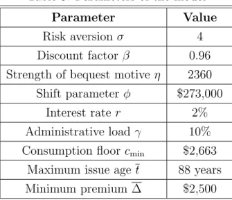
The discount factor β was set to 0.96, which is a standard value for calibrated life-cycle models. For preference parameters σ, η, and φ, and the minimum consumption floor cmin I used structural estimates from the DFJ study. Later on I report results for several alternative values of the coefficient of risk aversion and the discount factor. Table 5 summarizes all the parameter values.
Table 5: Parameters of the model
Parameter Value
Risk aversion σ 4
Discount factor β 0.96
Strength of bequest motive η 2360 Shift parameter φ $273,000
Interest rate r 2%
Administrative load γ 10% Consumption floor cmin $2,663
Maximum issue age t 88 years
Minimum premium ∆ $2,500
5.3
Initial distribution
Initial wealth (k0) and preexisting annuity holdings (n0) that individuals start their retirement with are calibrated from the AHEAD dataset. Individuals in the model start their retired life at age 70, so I used the cohort aged 69-76 in 1993 to calibrate initial wealth. The sample used for calibration includes only retired individuals who were single (divorced, separated or never married) at the time of the survey. The total number of observations is 1,114.
Initial financial wealth (k0) includes the value of housing and real estate, vehicles, value of business, IRAs, Keoghs, stocks, bonds, checking, and saving and money market accounts, less mortgages and other debts. Preexisting annuity holdings (n0) correspond to annuity-like income that an individual is entitled to receive during his retirement years. To measure annuity-like income, I sum the values of Social Security benefits, DB
pensions, and annuities that individuals receive each year and then take the average over all years that individuals are observed in the data. This measure of preexisting annuity income also proxies permanent income (I). Since both Social Security benefits and DB payments are closely linked to lifetime earnings, this provides a good approximation of permanent income.
The joint distribution of retirees over k0 and n0 was estimated using two-dimensional kernel density.
6
Results
This section presents results for different versions of the model above. It starts with the analysis of a model without medical expenses (zt = 0 for ∀ t), bequest motives
(η = 0), or minimum annuity purchase requirements (∆ = 0) and with full information annuity pricing. This simplified model is used to study annuitization decisions for people in different income quintiles, given heterogeneity in life expectancy and initial wealth holdings.
This simplified version of the model is then augmented with, first, deterministic and, second, uncertain medical expenditures. The model with uncertain medical expenditures is the baseline for further comparisons.
The following features of the baseline model are then changed one at a time. First, I drop full information assumption and require insurance firms to price annuities according to scenario two, the asymmetric information scenario. Second, I allow for a bequest motive. Third, I increase the consumption minimum floor. Fourth, I assume housing wealth is completely illiquid. Fifth, I consider the effect of the restrictions on minimum annuity purchase.
6.1
Simplified version of the model: no medical expenses
The model considered here only allows for lifespan uncertainty and preannuitized wealth coming from Social Security and DB pension plans. There are no medical expenses, bequest motives, minimum annuity purchase requirements, or unfair annuity pricing.
To illustrate the intertemporal decision process, Figures 1 and 2 show the general pattern of annuity purchases for individuals who were given initial wealth and annu-ity holdings that correspond to the median values in the initial distribution for each permanent income quintile. Several things can be noticed in the graph.
First, people buy annuities only once in the first period. It can be shown (see Pashchenko, 2010) that, under certain conditions, the one-time purchase of annuities in the first period is a general result. The conditions under which this result holds are
70 75 80 85 90 95 0 0.5 1 1.5 2 2.5 3 3.5 4 4.5 5 age
annuity income, thousands
Annuity purchased at each age
1st quintile 2d quintile 3d quintile 4th quintile 5th quintile
Figure 1: Annuities purchased by people in good initial health 70 75 80 85 90 95 0 0.5 1 1.5 2 2.5 3 3.5 4 4.5 5 age
annuity income, thousands
Annuity purchased at each age
1st quintile 2d quintile 3d quintile 4th quintile 5th quintile
Figure 2: Annuities purchased by people in bad initial health
the following:
- There is no uncertainty except the time of death - Medical expenditures are constant
- β(1 +r)<1
- n0 − z > cmin or k0 + n0 −z > q1(cmin − n0 −z), where z is value of medical expenditures that doesn’t change over time.
The last condition insures that an individual is already guaranteed income net of medical expenditures that exceeds the minimum consumption floor or can afford to get the equivalent stream of income by buying an annuity in the first period.
The intuition behind this theoretical result is as follows. There are two ways to finance an annuity purchase: using financial wealth or existing annuity income. The second way would imply increasing consumption profile, which is not optimal given β(1 +r) < 1. Thus, if an individual buys an annuity, he will use his financial wealth. If the individual waits to buy annuities, he has to save in bonds. But this strategy is dominated by buying annuities from the start, because over the long-run an annuity brings a higher return.
Second, the amount of annuity purchased is increasing with income quintile. People in the highest income quintile who start their retirement in good health buy a stream of annuity income equal to almost $2,500 per year. People in the second income quintile buy a stream of annuity income equal to only $700. The median annuity purchases of retirees in the lowest quintile is almost zero.
Third, people who start their retirement in bad health invest less in annuities than people whose initial health is good. While healthy retirees in the highest income quintile buy annuity income equal to almost $2,500, retirees in bad health in the same income quintile buy annuity income of only $1,700. This difference is explained by two factors.
First, people in bad health have lower life expectancy. Second, people in bad health start their retirement with lower wealth.
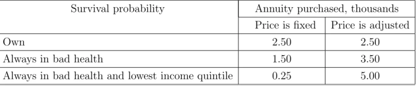
To isolate the effect of the survival probability on annuity demand, I run two coun-terfactual experiments. In the first experiment, an individual who starts his retirement in good health was given the survival probability of a person whose health is always bad without changing initial wealth. In the second experiment, the survival probability was set to be that of someone who is always in bad health and in the lowest income quintile. The results of these experiments are presented in the first column of Table 6 for retirees in the top income quintile (the results for other quintiles are similar)
Table 6: Impact of survival probability on annuity demand, top PI quintile Survival probability Annuity purchased, thousands
Price is fixed Price is adjusted
Own 2.50 2.50
Always in bad health 1.50 3.50
Always in bad health and lowest income quintile 0.25 5.00
Everything else being equal, the reduction in survival probability decreases demand for annuities: in the first experiment, the annuity purchase decreases from $2,500 to $1,500 and in the second experiment, to $250. It is important to note, however, that in these experiments, the change in the survival probability did not have any effect on price, which was fixed at the level of a price for a retiree whose initial health is good. In another set of experiments, I allow the annuity price to adjust to changes in the survival probability. The results are presented in the second column of Table 6. In this case, the decrease in survival probability actually increases demand for annuities: in the first experiment, the amount of annuity bought increases from $2,500 to $3,500 and in the second, to $5,000. This is explained by the fact that a decrease in the survival probability triggers two effects: it increases the effective discount factor, making people care less about future consumption, and it decreases the price for annuities, making future consumption more affordable. The income effect from decreasing price turns out to be more powerful.
Given that insurance firms have full information about the annuity buyer in the sim-plified version of the model considered in this subsection, prices are based on individual survival probabilities. Individuals who start their retirement in bad health, face lower annuity prices and this should increase their demand for annuities. Lower demand for annuities on the part of this group results from the fact that they have less initial wealth, not a lower survival probability.
Apart from the amount of annuity purchased, another dimension to consider is how many people do invest in annuities. The first column of Table 7 shows the percentage of retirees in each income quintile who have non-zero investments in annuities. The first thing to notice is that the overall participation rate is very high: 75.3% of retires invest in annuities, despite the fact that they already have part of their wealth annuitized through Social Security and DB pension plans.
Table 7: Participation in annuity market: model without medical expenses
Income quintile Percentage
With preannuitized wealth Preannuitized wealth removed
All 75.3 91.0 1 51.0 85.3 2 86.7 100.0 3 78.6 100.0 4 81.3 100.0 5 75.5 100.0
For comparison, the second column of Table 7 presents results for the case where individuals do not have any preannuitized wealth. More specifically, initial wealth k0 was increased by the amount q1n0 and annuity holdings n0 were set equal to zero. In other words, retirees were given additional liquid wealth which corresponds to the market value of the annuity income they are entitled to. In this case the overall participation rate increases to 91%. Except for the bottom income quintile, all retirees buy annuities. The fact that around 15% of people in the first quintile do not invest in annuities is explained by the fact that they rely on the minimum consumption floor provided by the government. The comparison between the first and second columns of Table 7 shows that preannuitized wealth has a significant effect on the annuity market participation rate. However, even in the presence of Social Security and DB pension plans, the interest in private annuities is still high.
Another important observation is that in the model with preannuitized wealth and no medical expenses, we do not see the monotonic relationship between the annuity market participation rate and the income quintile that can be observed in the data. On the contrary, the participation rates are lowest for people in the highest (fifth) and the lowest (first) income quintiles. Around 75% of the retirees in the fifth income quintile choose to invest in annuities and among those in the first income quintile, the rate is 51%. For comparison, among people in the second income quintile, participation is around 87%. The relatively low participation rate of the highest income quintile is not surprising in
this environment. People in the highest income quintile have a considerable amount of annuity income already and, given the absence of precautionary motives, they choose not to invest ny more in annuities.
Table 8: Share of annuity-like income in available resources
Quintile Retirees who Retirees who bought annuity didn’t buy annuity
1 20.9 36.3
2 36.6 94.7
3 33.8 90.8
4 32.3 91.4
5 24.6 88.1
In general what matters for annuity demand in the environment with no uncertainty except the time of death, no bequest motives, and actuarially fair prices is the combi-nation of liquid and annuitized assets that people have (see Pashchenko, 2010). The necessarily conditions for a retiree to invest in an annuity are that the annuity income he is entitled to is relatively small and the amount of liquid wealth is relatively big. Ta-ble 8 shows the share of annuity income in total amount of availaTa-ble resources n0
k0+n0 separately for people who bought annuities and those who did not. Those retirees in the top four income quintiles who decide not to invest in annuities have few resources ex-cept from annuity income: the ratio of annuity income to total available funds is around 90%. For people who chose to invest in annuities this ratio is much lower: it does not exceed 40%. The only quintile where this is not true is the bottom one. Even those people who choose not to invest in annuities have this ratio below 40%. It is important to note that for this quintile, the actual annuity income that they take into account is the income from the government-provided means-tested transfers. The majority of this group (around 68%) cannot afford to buy an annuity that will guarantee them income higher than the consumption minimum floor3.
6.2
The effect of medical expenditures
6.2.1 Deterministic medical expenditures
The next question is how the pattern of annuity holdings changes when medical expen-ditures are introduced. Figures 3 and 4 show the results for the case when retirees are
3Note, that to buy income equal to the minimum consumption floor, people have to pay upfront
facing medical expenditures that are deterministically increasing over time. That is to say, ψt in expression (1) is set to zero and the mean of medical expenditures is adjusted to match the mean in the stochastic case4.
70 75 80 85 90 95 0 0.5 1 1.5 2 2.5 3 3.5 4 4.5 5 age
annuity income, thousands
Annuity purchased at each age
1st quintile 2d quintile 3d quintile 4th quintile 5th quintile
Figure 3: Deterministic medical expenses: annu-ities purchased by people in good initial health
70 75 80 85 90 95 0 0.5 1 1.5 2 2.5 3 3.5 4 4.5 5 age
annuity income, thousands
Annuity purchased at each age
1st quintile 2d quintile 3d quintile 4th quintile 5th quintile
Figure 4: Deterministic medical expenses: annu-ities purchased by people in bad initial health
The pattern of annuity purchases changes significantly compared to the case of no medical expenditures. People still buy annuities at the beginning of retirement but they also increase annuity holdings towards the end of life. The retirees now have to save more because they have to finance not only their consumption but also medical expenditures that are increasing steeply over time. In this case, retirees use their annuity income to buy more annuities. The survival probability and, thus, the price of an annuity are decreasing with age and, as annuities become cheaper, they are more actively used to finance medical expenses.
The fraction of retirees involved in the annuity market increases in the presence of de-terministic medical expenses. The second column of Table 9 presents participation rates in the beginning of retirement and the second column of Table 10 present participation rates in the last period when individuals are allowed to buy annuities (88 years). The participation rate at age 70 goes up from 75 to 86% and the participation rate at age 88 increases from 0 to 77%.
Thus, if anything, the presence of deterministic medical expenditures increases de-mand for annuities in a significant way. This means that medical expenditures by them-selves cannot be an explanation for the annuity puzzle. The next section will consider how the stochastic component of medical expenditures affects annuity demand.
4The term ”deterministic” was chosen to emphasize the absence of the stochastic component. There
Table 9: Participation in annuity market at age 70: effect of medical expenses Medical expenses
Income quintile None Deterministic Uncertain
All 75.3 86.1 76.3 1 51.0 32.4 40.7 2 86.7 90.2 80.7 3 78.6 100.0 83.8 4 81.3 100.0 85.9 5 75.5 99.6 84.8
Table 10: Participation in annuity market at age 88: effect of medical expenses Medical expenses
Income quintile None Deterministic Uncertain
All 0.0 77.2 72.1 1 0.0 0.9 11.1 2 0.0 63.8 58.9 3 0.0 50.5 76.3 4 0.0 99.4 81.9 5 0.0 99.2 85.8
6.2.2 Uncertain medical expenditures
Introduction of the uncertain medical expenditures enforces the pattern of annuity pur-chases observed in the previous experiment: the demand for annuities increases substan-tially in the advanced ages (see Figures 5 and 6). To understand why retirees now buy even more annuities in advanced ages, one has to remember that the stochastic compo-nent of medical expenditures is highly persistent. Thus, with some probability retirees will face much higher medical expenses than in the deterministic case.
The participation rate drops compared to the case of deterministic medical expendi-tures but still stays higher than in the case of no medical expendiexpendi-tures (see third columns of Table 9 and Table 10). Thus, uncertainty in medical expenses results in two things. Some retirees, mostly in the lower income quintiles, give up on fully financing their health costs and decrease participation in the annuity markets. At the same time, retirees who choose to self-insure against medical shocks increase their annuity holdings.
One interesting result is that in the first retirement period, the introduction of deter-ministic medical expenses increases participation in the annuity market in each quintile
70 75 80 85 90 95 0 0.5 1 1.5 2 2.5 3 3.5 4 4.5 5 age
annuity income, thousands
Annuity purchased at each age
1st quintile 2d quintile 3d quintile 4th quintile 5th quintile
Figure 5: Uncertain medical expenses: annuities purchased by people in good initial health
70 75 80 85 90 95 0 0.5 1 1.5 2 2.5 3 3.5 4 4.5 5 age
annuity income, thousands
Annuity purchased at each age
1st quintile 2d quintile 3d quintile 4th quintile 5th quintile
Figure 6: Uncertain medical expenses: annuities purchased by people in bad initial health
except the bottom one, where participation actually decreases. Introduction of uncer-tain medical expenses decreases participation rates in each quintile except the bottom one, where participation increases. This behavior of people in the bottom quintile is explained by their reliance on government transfers. The introduction of deterministic medical expenses makes it easier to qualify for the means-tested transfers. If medical ex-penses have a persistent stochastic component, some groups of people may not meet the requirements for receiving government transfers in case their realized medical shocks are small. Thus, they have to finance their old age consumption themselves so they increase annuity market participation.
Another dimension to consider is the share of annuity investment in retirees’ portfo-lios. Table 11 shows this percentage for individuals with median wealth holdings at the beginning of retirement for three cases: no medical expenses, deterministic, and uncertain medical expenses.
Table 11: Percentage of annuity investment in retiree’s portfolio at age 70 Medical expenses
Income quintile None Deterministic Uncertain
1 0.0 0.0 0.0
2 100.0 100.0 73.0
3 100.0 100.0 92.5
4 100.0 100.0 81.8
The median retiree in the bottom income quintile does not invest in annuities in all three cases. Among other quintiles, only retirees in the fifth quintile did not save entirely in annuities in the case of no medical expenses. This means that since people in this quintile are entitled to big annuity income already, they prefer to decumulate part of their financial wealth in several years as opposed to a lifetime investment in annuity. In the case of deterministic medical expenses, annuities clearly dominate bonds for each income quintile. Finally, in the case of uncertain medical expenses, individuals prefer to hold part of their wealth in liquid form in order to be able to finance transitory medical shocks.
6.2.3 Summary of the effect of medical expenses
In general, if anything uncertain medical expenditures make the annuity puzzle harder to explain. Uncertain medical expenditures do decrease the annuity market participation rate in the lower income quintiles but, in the aggregate, this is more than compensated for by the increase in the demand for annuities from the high income quintiles. People who can afford to finance their medical expenses will do it at least partially through buying annuities. The annuity pays out in a state when the individual is old and alive, and it coincides with the state when he is likely to have high medical expenses. Thus, insuring medical expense risk and insuring longevity risk become complementary. This result is consistent with the conclusion of Pang and Warshawsky (2008) that medical expenses increase retirees’ investment in annuities.
The version of the model with uncertain medical expenses, fair prices, and no bequest motives is the baseline for comparison for all further experiments. The pattern of annuity purchased we observed in Figures 5 and 6 is robust to all subsequent changes in the baseline model, so I omit graphs of annuity purchase in retirement in the rest of the analysis.
6.3
Effect of adverse selection
In this section, I consider a version of the model in which insurance firms price annuities according to the asymmetric information scenario. This means they do not observe any characteristics of the annuity buyer except age. In this case, there exists one pooling price that is above what is actuarially fair for people with high mortality and below what is actuarially fair for people with low mortality. Since mortality is negatively correlated with permanent income, this means that in the pooling equilibrium, higher income quintiles will face better prices and thus get an implicit subsidy from low income quintiles. Table 12 provides a quantitative assessment of this subsidy. For people in the lowest income quintile and bad health, the pooling equilibrium price is around 73% higher than the
price they face if the insurance firms observe their mortality. On the other extreme, people in the highest quintile and in good health pay 13% less for annuities than in the full information equilibrium.
Table 12: Percentage change in price in pooling equilibrium compared to full information equilibrium
Income quintile Bad health Good health
1 73.2 25.7
2 53.5 14.0
3 35.7 3.7
4 20.1 -5.3
5 6.8 -13.1
As a result, the participation of high income quintiles in the annuity market increases and the participation of low quintiles decreases. Table 13 compares the participation rates with the baseline model. In the bottom income quintile, the fraction of people buying annuities at age 70 drops from 40.7% to 30.8%. In the highest quintile, this number increases from 84.8% to 93.5%. The decline in participation rates among low income quintiles is partially offset by the increase in participation rates among low quintiles. Thus, the overall effect of the adverse selection is quite small: in the pooling equilibrium the percentage of people involved in the annuity market at age 70 decreases by less than 4% compared to the baseline model.
Table 13: Participation in annuity market at age 70: baseline model vs. model with adverse selection
Income quintile Baseline Adverse selection
All 76.3 72.5 1 40.7 30.8 2 80.7 63.1 3 83.8 74.7 4 85.9 89.9 5 84.8 93.5
6.4
Effect of bequest
An annuity is a financial instrument that pays out only in a state when the individual is alive. Bequest motives make individuals care about a state when they are not alive and thus decreases the attractiveness of annuities. In theory very strong bequest motives can drive demand for annuities to zero. However, the empirical evidence suggests that a bequest is a luxury good; moreover, only saving decisions of people in the highest income quintile get affected by bequest motives in a significant way (De Nardi, French, and Jones, 2009).
To get some idea of the effect of bequest motives, this section uses recent estimates of De Nardi, French, and Jones (2009). Using the AHEAD dataset, DFJ found that the strength of the bequest motive (η) is equal to 2360 and the shift parameter (φ) is equal to $273,000. The easiest way to understand the intuition behind these parameters’ values is to consider a two-period deterministic model where an agent lives for one period and dies with certainty in the second period. In this case, using the estimated values forη and φ, one can compute that only individuals with wealth above $38,000 will leave a bequest. Once the bequest motive becomes operative, its effect is very strong: 88 cents of every additional dollar of wealth will be bequeathed (see DFJ, 2009).
Table 14 illustrates the effect of bequest motives on participation rates: overall the percentage of retirees involved in the annuity market decreases by around 4%. This decrease mostly comes from the highest income quintile. While participation rates for individuals in the first four quintiles are hardly affected, the fraction of people buying annuities in the fifth income quintile decreases by almost 16%, from 85.8 to 69%. This is not surprising given the high value of the shift parameter φ: only people in the highest income quintile are significantly affected by a bequest motive.
Table 14: Participation in annuity market at age 70: baseline model vs. model with bequest motives
Income quintile Baseline Bequest motive
All 76.3 71.9 1 40.7 40.6 2 80.7 79.7 3 83.8 83.2 4 85.9 85.7 5 84.8 69.0
6.5
Effect of minimum consumption floor
The consumption minimum floor provides alternative annuity income, and the question is how well does it substitute for a private annuity. In the baseline model of this study, the
government guaranteed consumption minimum floor was set to be equal to $2,663. This number is on the low side of what is commonly used in the literature (see Kitao and Jeske, 2009, and Kopecky and Koreshkova, 2009). Table 15 demonstrates how participation in the annuity market changes when the consumption floor is raised to $6,000.
Table 15: Participation in annuity market at age 70: baseline model vs. model with cmin= $6000
Income quintile Baseline cmin = $6000
All 76.3 53.1 1 40.7 8.6 2 80.7 28.8 3 83.8 61.5 4 85.9 73.5 5 84.8 82.9
The increase in the consumption minimum floor has a significant effect on the overall participation rate: it drops from 76.3 to 53.1%. This decrease mainly comes from the three bottom income quintiles - the top two quintiles are affected much less. While in the first quintile, an increase in the consumption minimum floor leads to a decline in the participation rate from 40.7 to 8.6%, in the highest quintile the participation rate goes down from 84.8 to 82.9%. This asymmetric effect is not surprising. People in the highest quintile start their retirement with annuity income that is significantly higher than the consumption minimum floor. For them, the probability of qualifying for means-tested government transfers is low: it happens only if they get hit by a bad sequence of medical shocks. Hence, the size of the consumption minimum floor has a small effect on their decision to annuitize. People in the lower quintiles have more chances to rely on government transfers and the increase in public longevity insurance has a big effect on their demand for private annuities.
6.6
Effect of illiquid housing
In the next version of the model, I assume that housing wealth is completely illiquid. In other words, each person’s total initial wealth is replaced with his total non-housing wealth. The assumption that retirees cannot use their housing wealth even to finance medical expenses is the other extreme from the assumption maintained before that house-holds can consume out of their housing wealth. It has been shown (Walker, 2004) that housing wealth in retirement is not used to finance consumption; however, it may be
used to finance catastrophic medical expenditures. Given computational difficulties with treating housing wealth as a separate state variable, this paper considers two alternative assumptions of perfect liquidity and absolute illiquidity of housing wealth. This may give some idea about the magnitude of the bias of imposing any assumption of this sort. What is important for this study, however, is that housing wealth is not equal to non-housing wealth in terms of the cost of converting it into annuity.
Table 16 shows the percentage of retirees involved in the annuity market if housing wealth is assumed to be illiquid. The ban on using housing wealth decreases the partici-pation rate though the effect is not big; on average only around 3% of retirees leave the market. Illiquidity of housing wealth uniformly affects all quintiles, though the biggest effect it has is on retirees in the bottom quintile: their participation rate drops by 10%. This big effect is explained by the fact that for this group of people housing constitutes a major part of their retirement wealth. In the next section, I will show that the illiquidity of housing wealth has a much bigger effect on the participation rate once a minimum annuity purchase requirement is introduced.
Table 16: Participation in annuity market at age 70: baseline model vs. model with illiquid housing
Income quintile Baseline Illiquid housing
All 76.3 73.2 1 40.7 30.5 2 80.7 74.9 3 83.8 78.6 4 85.9 80.3 5 84.8 77.5
6.7
Effect of minimum purchase requirements
In this section, I assume the insurance firms set a minimum annuity purchase requirement equal to $2,500. The results of introducing a minimum purchase requirement in the baseline model are presented in Table 17. The decline in participation rates is very noticeable; the percentage of people involved in the annuity markets drops from 76.3 to 39.9%. The effect of a minimum purchase requirement on the participation rate becomes even bigger once housing wealth is assumed to be totally illiquid (third column of Table 17). The participation in annuity market at age 70 drops to 24.2%.
Table 17: Participation in annuity market at age 70: baseline model vs. model with minimum purchase requirement
Income quintile Baseline Minimum purchase
Liquid housing Illiquid housing
All 76.3 39.9 24.2 1 40.7 23.9 11.2 2 80.7 32.5 16.1 3 83.8 35.4 18.6 4 85.9 43.1 23.7 5 84.8 57.4 36.4
The large effect of the restriction on minimum investment in annuity on the partic-ipation rates results from the fact that a lot of retirees involved in the annuity market invest only small amounts. Even in the highest income quintile, for a considerable group of retirees the optimal amount of investment in annuities is below the minimum one: the participation in this quintile decreases from 84.8 to 57.4% in the case with liquid housing. This reduction is accounted for by people whose financial wealth is relatively small compared to their preexisting annuity income.
Given that on average retirees are willing to participate in the annuity market but are not willing to invest a lot, one question to ask is: how much do individuals value access to the annuity market? Table 18 shows how much a median retiree has to be compensated in terms of the percentage of consumption if he loses access to the annuity market.
Table 18: Value of annuity market for median retiree in each income quintile (in percent-age of consumption)
Income quintile Good health Bad health
1 0.0 0.0
2 2.4 0.7
3 2.3 0.3
4 6.3 2.8
5 8.9 7.3
Not surprisingly, the value of the annuity market for retirees increases with income quintile and health status. If a median retiree in the lowest income quintile is indifferent between having access to the annuity market or not, for a retiree in good health and in the highest income quintile the loss of opportunity to invest in annuities is equivalent to
8.9% of consumption. In general for people in good health and in high income quintiles the opportunity to have access to the annuity market is very valuable. Annuities bring higher returns over the long run and can help to finance medical expenses late in life. However, the amount of money that retirees can actually spare to invest in annuities is not big. The issue of liquidity constraints is accentuated by the need to keep part of the wealth as a buffer stock against medical shocks and the impossibility of using housing wealth.
6.8
Summary
The quantitative effect of the different explanations for non-annuitization is summarized in Table 19. In terms ofoverall participation rates, three factors have the largest effects: preannuitized wealth, minimum purchase requirement and consumption minimum floor. In terms of participation ratesby quintile, the consumption minimum floor affects mostly people in low quintiles while the impacts of minimum purchase requirement and preann-utized wealth are approximately uniform. Bequest motives have a significant effect only on people in the highest income quintile. The impact of illiquidity of housing wealth is large only in combination with a minimum purchase requirement. Adverse selection and medical expenses have significant effects on participation rates in each quintile, but these effects have the opposite sign for low- and high-income group. For people in low income quintiles, both medical expenses and adverse selection reduce participation in the annuity markets, while for people in high income quintiles the effect goes the other way.
Table 19: Quantitative importance of different factors behind non-annuitization
Factors Impact on low quintiles Impact on high quintiles Overall effect Preannuitized wealth Big (negative) Big (negative) Big (negative)
Medical expenses Big (negative) Big (positive) Small (positive) Adverse selection Big (negative) Big (positive) Small (negative)
Bequest None Big (negative) Small (negative)
Consumption floor Big (negative) Small (negative) Big (negative) Illiquid housing Small (negative) Small (negative) Small (negative)
Minimum premium Big (negative) Big (negative) Big (negative)
6.9
Combined effect
Now that the separate effects of different factors behind non-annuitization are quantified, the next step is to evaluate how much all these factors combined can contribute to the
annuity puzzle. To do this I consider the full version of the model: in this version insurance firms are assumed to price according to the asymmetric information scenario and restrict the minimum amount of annuity purchase. Retirees face stochastic medical expenses, have bequest motives, and cannot use their housing wealth. The consumption floor guaranteed by the government is set to be equal to $6,000 per year. Table 20 compares annuity market participation rates at age 70 produced by the full model with the baseline model and with participation rates observed in the data for people aged from 70 to 80 years old.
Table 20: Participation in annuity market at age 70: baseline model vs. model with all impediments to annuitization
Income quintile Baseline Full version Data
All 76.3 19.6 6.2 1 40.7 1.9 1.2 2 80.7 6.5 1.3 3 83.8 12.8 2.7 4 85.9 20.8 4.5 5 84.8 35.3 13.0
As can be seen the model, combining different factors behind non-annuitization goes a long way in explaining low participation rates in the annuity market compared to the baseline model. However, the predicted participation rates are still higher than those observed in the data.
Another way to look at the performance of the model is to compare prices it produces with the ones observed in the data. Figure 7 shows that prices in the model line up well with what we see in the data5, though the model underpredicts the real prices.
There are at least three explanations for this downward bias of the prices in the model. First, the model considers only single individuals, while real prices are based on the aggregate statistics that include couples. Second, the AHEAD dataset underrepresents wealthy individuals. Given that wealth is negatively correlated with mortality and that rich individuals tend to buy more annuities, the lack of wealthy individuals in the model biases the prices downwards6. Third, this paper makes assumption that insurance firms are perfectly competitive and sets administrative load to 10%. It may be that the markup
5The observed price corresponds to the price of a lifetime annuity with fixed income payment with
inflation adjustment. The quotes were obtained from Vanguard at www.aigretirementgold.com.
6This problem is accentuated by the fact that for the calibration of the initial distribution, the second
wave of the AHEAD dataset was used. This wave tend to significantly underreport asset holding ( see Rohwedder, Haider, and Hurd, 2004).
70 72 74 76 78 80 82 84 86 88 4 5 6 7 8 9 10 11 12 13 age
Price for unit of insurance contract ($)
Model Data
Figure 7: Prices in the model and in the data
insurance firms actually have is more than 10% due to higher administrative expenses or violation of the perfect competition assumption.
7
Conclusion
This study considers different explanations for the annuity puzzle in a quantitative het-erogeneous agent model. It shows that, in the absence of any impediments to annuiti-zation, all but the poorest retirees buy annuities. Social Security and DB pension plans significantly decrease the annuity market participation rate but it still remains high.
Uncertain medical expenses increase demand for annuities because health expendi-tures are increasing with age: the state of being old and alive coincides with the state of being old and having to pay high medical costs. Thus, insurance against longevity risk and insurance against medical costs uncertainty compliment each other.
Adverse selection decreases demand for annuities for people in low income quintiles because their mortality is high and in equilibrium they face unfair prices. However, the equilibrium price is not high enough to completely crowd high mortality types out of the market. Thus, in pooling equilibrium people in high-income quintiles face lower prices, which increases their demand for annuities.
The quantitative effect of bequest motives is not big because it affects the demand for annuities only for those in the highest income quintile. Public longevity insurance provided through various means-tested transfers plays a big role in reducing demand for private annuities from the low and middle income quintiles.
In general, people place a high value on the opportunity to invest in annuities. How-ever, the amount of annuities retirees are actually buying is small. This is because
annuities bring returns for many years and the upfront investment even when buying a small stream of annuity income is not trivial. When insurance firms restrict the minimum amount an individual can invest in an annuity, it substantially decreases the number of retirees in the market, especially if housing wealth cannot be annuitized.
8
Appendix
8.1
Robustness check
This section checks the sensitivity of results to changes in two parameters: discount factor (β) and risk aversion (σ). Table 21 compares participation rates in the annuity market with the baseline model when β is first raised to 0.98 and then decreased to 0.8. Note, that in the first experiment β was increased to the point when β(1 +r) = 1.
Table 21: The sensitivity of participation rates to change in discount factor Income quintile Baseline β = 0.98 β = 0.80
All 76.3 81.2 43.0 1 40.7 43.9 26.4 2 80.7 85.1 44.1 3 83.8 90.4 45.8 4 85.9 90.1 47.2 5 84.8 89.9 48.3
Not surprisingly, an increase in the discount factor raises annuity market participation rates and a decrease in the discount factor has the opposite effect. Patient individuals save more and so they are more interested in annuities as one of the available saving options. The overall increase in the participation rate due to a higher discount factor is equal to 5%. When the discount factor goes down to 0.8, the participation rate drops almost twice. In general, an increase in the discount factor makes the annuity puzzle harder to explain, though the effect is not big for ranges where β(1 +r)≤1.
In the next experiment, risk aversion was first set to 2 and then raised to 4. Table 22 compares the results of these experiments with the baseline model. When risk aversion decreases, agents want to save less and, thus, they buy less annuities. An increase in risk aversion has the opposite effect. Higher risk aversion makes the annuity puzzle harder to explain, but again, the effect is not big.