Doctoral Dissertations University of Connecticut Graduate School
8-12-2015
Dynamic Modeling of Multivariate Counts
-Fitting, Diagnostics, and Applications
Volodymyr Serhiyenko
University of Connecticut - Storrs, [email protected]
Follow this and additional works at:https://opencommons.uconn.edu/dissertations Recommended Citation
Serhiyenko, Volodymyr, "Dynamic Modeling of Multivariate Counts - Fitting, Diagnostics, and Applications" (2015).Doctoral Dissertations. 858.
– Fitting, Diagnostics, and Applications
Volodymyr Serhiyenko, Ph.D. University of Connecticut, 2015
ABSTRACT
An adequate statistical methodology is required for modeling multivariate time series of counts. The proper specification of the underlying distribution in such model-ing could be very challengmodel-ing, as it should account for the possibility of overdispersion, an excessive number of zero values, positive and negative association between counts, etc.
This dissertation is focused on modeling multivariate time series of counts as a function of location-specific and time-dependent covariates. The Bayesian framework for estimation and prediction is discussed. We focus on Markov chain Monte Carlo (MCMC) methods for fully Bayesian inference and the Integrated Nested Laplace Approximation (INLA) for fast implementation of approximate Bayesian modeling which is especially useful for large data sets.
The dissertation has three main contributions. First, we propose a dynamic model that combines time series compositional modeling with dynamic modeling for counts. This approach is applied to the problem of transportation engineering. We investigate the temporal behavior of injury severity levels as proportions of all pedestrian crashes in each month, taking into consideration effects of time trend, seasonal variations and
VMT (vehicle miles traveled).
Second, this dissertation discusses a hierarchical multivariate dynamic modeling framework. The use of a multivariate Poisson (MVP) sampling distribution is dis-cussed. We show that the use of such distribution enables us to model the association between components of the multivariate response vector over time. This approach is illustrated using data from ecology on gastropod abundance in Puerto Rico.
Finally, we propose a level correlated model (LCM) to account for the association among the components of the response vector. This multivariate model accounts for overdispersion as well as for positive and negative association between counts. The flexible LCM framework allows us to combine different marginal count distributions and to build a dynamic model for the vector time series of counts. We comprehensively discuss the lower and upper limits for the association between the components of the response vector of counts. We employ the proposed modeling to ecology and marketing examples and discuss the results.
– Fitting, Diagnostics, and Applications
Volodymyr Serhiyenko
M.S. Mathematics, The City College of New York, 2010 B.S. Mathematics, Lviv Ivan Franko National University, 2007
A Dissertation
Submitted in Partial Fulfillment of the Requirements for the Degree of
Doctor of Philosophy at the
University of Connecticut
Volodymyr Serhiyenko
Doctor of Philosophy Dissertation
Dynamic Modeling of Multivariate Counts
– Fitting, Diagnostics, and Applications
Presented by
Volodymyr Serhiyenko, B.S. Math., M.S. Math.
Major Advisor Nalini Ravishanker Associate Advisor Xiaojing Wang Associate Advisor John N. Ivan University of Connecticut 2015 ii
Since first I came to Storrs, I could not imagine that in five years I will be leaving it with so much unforgettable memories. It was a challenging, nevertheless incredible and delightful period of my life. I would like to acknowledge all the great people that I was lucky to meet during my PhD journey at the University of Connecticut.
First of all, I would like to express my highest gratitude to my major advisor, Professor Nalini Ravishanker. Without any hesitation I can say that she has been responsible for my success during these five years. Professor Ravishanker shared her endless knowledge and gave important and crucial advise during our countless meetings, Skype talks, projects, and conferences. Her patience, enthusiasm, encour-agement, and critique helped me to expand my research in numerous directions. I could not have imagined having a better advisor and mentor for my PhD study.
I would like to express my very great appreciation to my associate advisors Pro-fessor Wang and ProPro-fessor Ivan for all of their vital input in my research. Their comments and guidance helped me a great deal in the writing of this work and en-hanced my dissertation in various ways.
I would like to offer my special thanks to all faculty members in the Department of Statistics at University of Connecticut. Especially, I want to express my sincere appreciation to Professor Nitis Mukhopadhyay, Professor Cyr M’Lan, Professor Zhiyi Chi, and Dr. Naitee Ting for all their support and inspiration during my graduate study. I also want to thank Tracy Burke and Megan Petsa for the immense work that
they put behind my five years of study.
My sincere thanks go to Professor Mike Willig and Professor Rajkumar Venkatesan for providing data and expert opinions in the ecology and marketing data analysis examples. I’m also very fortune to have met and worked with great classmates and colleagues from Statistics, Ecology, and Civil Engineering departments.
I am extremely grateful to my mother Oleksandra Serhiyenko, my father Anatoliy Serhiyenko, my sister Nataliya Lyakhovych and all of her family. They always support me in all of my endeavors. Also, I want to thank my newly acquired Nechyporenko family for treating me like their own son.
Lastly and the most importantly, I want to thank my wife, Khrystyna Serhiyenko. I cannot express in words how grateful I am for having her by my side. Her uncondi-tional support and love are the most important drivers in my life. Together we had many ups and downs while in the graduate school, and now we are fearlessly waiting for a new chapter in our life.
Ch. 1. Introduction and Literature Survey 1
1.1 Univariate and Multivariate Modeling of Counts . . . 1
1.2 Count Time Series Modeling . . . 4
1.3 Contribution of this dissertation . . . 7
Ch. 2. Review of Bayesian and Approximate Bayesian Methods 11 2.1 Markov Chain Monte Carlo sampling algorithms . . . 11
2.2 Approximate Bayesian Inference through INLA . . . 14
Ch. 3. Dynamic Compositional Modeling of Pedestrian Crash Counts on Urban Roads in Connecticut 17 3.1 Motivation . . . 18
3.2 Dynamic Compositional Time Series Modeling . . . 22
3.2.1 Study Design . . . 22
3.2.2 Model Framework . . . 23
3.2.3 Model Estimation . . . 25
3.2.4 Discussion of Results . . . 29
3.3 Dynamic and Static Modeling of Pedestrian Crash Counts . . . 31
3.4 Predictions of Crash counts by Injury Severity Levels . . . 38
3.5 Discussion and Conclusions . . . 39
Ch. 4. Hierarchical Dynamic Models for Multivariate Times Series of Counts 42 4.1 Gastropod Abundance in the Luquillo Experimental Forest in Puerto Rico - Data Description . . . 43
4.2 Multivariate Poisson Distribution . . . 47
4.3 Hierarchical Multivariate Dynamic Model (HMDM) . . . 51 v
4.4 Model Selection and Prediction . . . 58
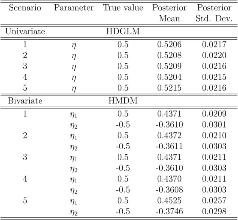
4.5 Simulated Data Results . . . 59
4.6 Analysis of Gastropod Counts . . . 63
Ch. 5. Dynamic Modeling of Multivariate Counts using Level Cor-related Models 70 5.1 Introduction . . . 70
5.2 Structure of Level Correlated Models . . . 71
5.3 Simulation Study . . . 77
5.3.1 Attainable Correlation in LCMs . . . 78
5.3.2 Estimation using INLA . . . 82
5.4 Gastropod Abundance Modeling Using LCM . . . 85
5.4.1 Data Description . . . 85
5.4.2 Model Framework . . . 87
5.4.3 Discussion of Results . . . 92
5.5 Marketing Modeling Using LCM . . . 98
5.5.1 Data Description . . . 98 5.5.2 Model Framework . . . 102 Ch. 6. Future Work 115
Appendix
117
Ch. A. Selected R code 118 A.1 Simulation of LCMs . . . 118A.2 Estimation of LCMs using R-INLA . . . 119
Bibliography 124
Introduction and Literature Survey
1.1
Univariate and Multivariate Modeling of Counts
The scientific literature is rich with regression modeling problems where the response variables are independent counts. The standard approach uses the Poisson distribu-tion as the response distribudistribu-tion and implements GLM (McCullagh and Nelder, 1989; Agresti, 2010). A serious drawback of the Poisson regression model is that it assumes a nominal dispersion, i.e., the mean is equal to the variance. In practice, count data are often overdispersed, i.e., show evidence that the variance is larger than the mean (Cameron and Trivedi, 1998).
The general solution to this problem is to assume that the Poisson mean is a mixture of fixed mean and a positive random variable. In this case, a nonnegative multiplicative random effect term is introduced into the model. The popular choice for the distribution of the random effect term is a gamma distribution. These types of models result in the negative binomial regression models (Cameron and Trivedi, 1998;
Winkelmann, 2008). In this context Bayesian inference has also been developed. Un-fortunately it involves computationally intensive Markov chain Monte Carlo (MCMC) algorithms, since there is no conjugate prior for regression coefficients when the un-derlying distribution is Poisson or negative binomial (Chib et al., 1998; Chib and Winkelmann, 2001; Winkelmann, 2008).
A lognormal distribution can also be used as a random effect in the Poisson model, which results in the Poisson-lognormal regression model as an alternative to the neg-ative binomial model (Breslow, 1984; Agresti, 2010). Moreover, Zhou et al. (2012) suggested that lognormal and gamma mixed negative binomial regression model for counts may fit the data better and has one extra degree of freedom to incorporate different kinds of random effects. They also developed Bayesian inference for that kind of model. The Conway-Maxwell-Poisson (COM-Poisson) was first introduced by Conway and Maxwell (1962) and just recently was used for modeling count data (Shmueli et al., 2005) in situations of under- or over-dispersion. The regression model was developed by Guikema and Coffelt (2008) for risk analysis and Lord et al. (2008) for traffic accident data. They gave a comprehensive discussion about non-Bayesian and Bayesian multivariate linear regressions, generalized linear regression models, as well as semi-parametric and non-parametric models.
The zero-inflated count models were introduced to handle data with a preponder-ance of zeros (Johnson and Kotz, 1969; Lambert, 1992) and applied in different fields through zero-inflated Poisson (ZIP) and zero-inflated negative binomial (ZINB) re-gression models (Shankar et al., 1997). The assumptions of zero-inflated models were discussed with respect to different applications in transportation engineering (Lord et al., 2005).
1967) for modeling applications was sparse until recently, possibly due to the com-plicated form of the probability mass function. Karlis and Meligkotsidou (2005) proposed the two-way covariance structured multivariate Poisson distribution which permits a more realistic modeling of multivariate counts for several practical appli-cations. Hu (2012) developed a Bayesian framework for regression and time series models based on the multivariate Poisson distribution. Nevertheless, this type of multivariate Poisson model assumes positive dependence between components of the vector-valued count variable, an assumption that is not realistic for several applica-tions. Further, the marginal mean and variance of each variable coincide and, thus, this model is not appropriate for overdispersed data sets. Karlis and Meligkotsi-dou (2007) proposed a finite multivariate Poisson mixture as an alternative class of models for multivariate count data. These models allow for both negative and pos-itive dependence and overdispersion. However, the computations can be very time consuming.
Another approach is the multivariate Poisson-lognormal model (Aitchison and Ho, 1989; Ma et al., 2008). The approach allows modeling dependence within the response vector for data that are possibly overdispersed. Although a Bayesian approach (Chib and Winkelmann, 2001; Ma et al., 2008) was developed for the regression model, the possibility of temporal dependence was not considered when the data are collected on different locations/segments over time. Moreover, a comprehensive description of properties for induced association between the components of the count response vector is missing from the literature. Although it was noted that the range of induced correlations is not as wide as that of the corresponding lognormal or normal distri-butions (Aitchison and Ho, 1989). It will be extremely useful to carefully quantify the values of the maxima and minima of the induced associations between the count
variables as a function of the marginal Poisson means and the variances and correla-tions of the components from the underlying lognormal distribution. Moreover, the possibility of using of the multivariate Poisson-lognormal regression in the case of time series and its extensions has not been discussed in the literature as well.
1.2
Count Time Series Modeling
The literature on count time series modeling includes observation driven models and parameter driven models. The generalized linear modeling (GLM) framework (Nelder and Wedderburn, 1972; McCullagh and Nelder, 1989) naturally combines the tradi-tional time series models such as the autoregressive models (AR), moving average models (MA), autoregressive moving average models (ARMA), seasonal ARMA, gen-eralized autoregressive conditional heteroskedasticity models (GARCH), etc.
The Poisson distribution is the first obvious choice of the underlying distribution for the time series modeling of counts under the GLM framework. In situations with overdisperssion, the negative binomial distribution can be considered. There are sev-eral count distributions that can be easily adopted for the time series setup such as the ZIP distribution (Lambert, 1992) and the truncated Poisson distribution (Fokianos, 2001). Excellent reviews of such time series models by Fokianos (2012), Tjøstheim (2012), and Davis et al. (2015) are valuable. We should note that the model esti-mation, diagnostics, and forecasting are implemented in various standard statistical packages and are readily available for the researches. The R package tscount gives a flexible framework for the estimation of count time series which follow generalized linear models. The R package glarma is another package that provides functions
for fitting generalized linear autoregressive moving average (GLARMA) models for discrete valued time series.
The model estimation can also be done using likelihood methods. Maximum likelihood inference for Poisson and negative binomial time series models has been developed by Davis et al. (2003), Fokianos et al. (2009), Fokianos and Tjøstheim (2012), and Christou and Fokianos (2014). Regression modeling for count time series using quasi-likelihood methods was discussed in Zeger (1998). Jørgensen et al. (1999) described analysis of longitudinal multivariate count data driven by a latent gamma Markov process using a state space approach. Song (2007) discussed marginal, condi-tional (random effects), and transicondi-tional approaches for analyzing correlated counts. Bayesian modeling of panel count data under the Poisson-lognormal model was dis-cussed in Chib et al. (1998), while Chib and Winkelmann (2001) disdis-cussed models with latent effects for correlated count data.
One approach to develop models for count time series is based on the thinning operator (Steutel and Van Harn, 1979), where the thinning operator is generated by counting series of Bernoulli-distributed random variables. McKenzie (1985) and Al-Osh and Alzaid (1987) independently developed the first-order integer-valued autore-gressive, INAR(1) model. McKenzie (2003) and Jung and Tremayne (2006) presented a good review of subsequent developments. The class of integer valued time series models based on thinning operations is more restrictive in its construction than mod-els based on the GLM framework (Tjøstheim, 2012). One of the drawbacks is that the autocorrelation is always positive. Also, nonlinear and multivariate extensions are not easily implemented under this framework (Drost et al., 2008; McKenzie, 2003). A good review of such models is given by Weiß (2008). Multivariate INAR models for counts were also discussed in Pedeli and Karlis (2011) and references therein.
For Gaussian dynamic linear models (DLMs), often referred to as Gaussian state space models, Kalman (1960) and Kalman and Bucy (1961) popularized a recursive algorithm for optimal estimation and prediction of the state vector, which then enables the prediction of the observation vector. The use of Gaussian state space models has gained in popularity since the books of Harvey (1990) and West and Harrison (1997). These books give comprehensive overview of the class of state space models from the classical and Bayesian perspectives. Hierarchical dynamic linear models (HDLMs) combine the stratified parametric linear models (Lindley and Smith, 1972) and the DLMs into a general framework, which have been particularly useful in econometric, education, and health-care applications. The Gaussian HDLM includes a set of one or more dimension reducing structural equations along with the observation equation and state (system) equation of the DLM (Gamerman and Migon, 1993). Landim and Gamerman (2000) further extended the Gaussian HDLM to a more general class of models where the response vector has a matrix-valued normal distribution. Count data models in the state space approach were discussed in Gamerman (1998), Durbin and Koopman (2000), Fr¨uhwirth-Schnatter and Wagner (2006), and Gamerman et al. (2013).
There is a considerable amount of literature on MCMC methods for non-Gaussian and non-linear state space models; see West et al. (1985), Carlin et al. (1992), Gordon et al. (1993), Song (2007). A detailed review of the MCMC methods can be found in Fearnhead (2011) and Migon et al. (2005). The simplest method updates the components of the states in the sequential fashion (Carlin et al., 1992; Geweke and Tanizaki, 2001). However, it is well known that this type of sampler may lead to slow mixing because of possible strong correlation between states. In such cases it is better to update the states in multiple instances as blocks of states or update the
entire state process at once (Shephard and Pitt, 1997; Carter and Kohn, 1994). We note that designing MCMC algorithms and tuning those can be cumbersome and time consuming, especially for multivariate state space models and regression and time series models for counts.
1.3
Contribution of this dissertation
In several application areas, we increasingly see the need for developing accurate statistical modeling approaches for time series of multivariate count responses. The response consists of an J-dimensional vector of counts that is observed at each of n
locations (or for each of n subjects) over T regularly spaced times. The objective of the statistical analysis is to understand stochastic temporal patterns in the response as a function of observed location (or subject)-specific and/or time-varying covariates. For instance, in ecology, understanding the causes and consequences of variation in the abundance of organisms as a function of topographical and environmental covariates has been a long-standing goal (Krebs, 1972; Scheiner and Willig, 2011). In business, a pharmaceutical firm may be interested in estimating and predicting the number of new prescriptions written by physicians of drugs from the firm and its competitors, as a function of the firm’s promotional activities (Venkatesan et al., 2012). In a problem in transportation engineering, it would be interesting to understand stochastic patterns in the temporal behavior of crash counts categorized by injury severity across a set of highway segments, as a function of roadway geometry, traffic volume, etc. (Hu et al., 2012). For such applications, the modeling described in this dissertation enables us to adequately incorporate dependence in the response over time as well as the
dependence between the components of the response vector.
This dissertation is focused on modeling multivariate time series of counts as a function of location-specific and time-dependent covariates. The proper specifica-tion of the underlying distribuspecifica-tion could be very challenging. It is well known that count data can exhibit overdispersion or underdispersion relative to the Poisson dis-tribution, or an excessive number of zero values. All of these situations cannot be adequately modeled by the Poisson distribution. The question that also arises is what framework to employ if the data require multivariate modeling. We focus on Markov chain Monte Carlo (MCMC) methods for fully Bayesian inference and the Integrated Nested Laplace Approximation (INLA) (Rue et al., 2009) for fast implementation of approximate Bayesian modeling for large data sets.
Chapter 3 describes the use of dynamic modeling of compositional time series derived from multivariate counts. We introduce a new model that combines the dy-namic and static models for counts and time series models of compositions under one framework. We investigate the temporal behavior of injury severity levels as proportions of all pedestrian crashes in each month, taking into consideration effects of time trend, seasonal variations and VMT (vehicle miles traveled). We describe a time series framework with vector autoregressions (VAR) for modeling and predicting compositional time series. Combining these predictions with predictions from a uni-variate statistical model for total crash counts enables us to predict pedestrian crash counts with different injury severity levels.
Chapter 4 gives details of a hierarchical multivariate dynamic model (HMDM) for a vector-valued time series of counts. We describe a fully Bayesian framework for estimation and prediction by assuming a multivariate Poisson (MVP) sampling distri-bution for the count responses. Our modeling incorporates the temporal dependence
as well as dependence between the components of the response vector.
The use of the MVP distribution also enables us to model the association between components as a function of subject/location and time specific covariates that can vary over time. We show that the use of MVP distributions enables us to model the association between components of the multivariate response vector over time. We apply this methodology to an example from ecology. Also, we discuss the computa-tional time associated with models that use MVP distributions. We note that the proposed models can not account for the negative association between the components of the vector-valued response counts.
In Chapter 5 we propose a level correlated model (LCM) to account for the as-sociation among the components of the response vector. This model for multivariate time series of counts accounts for overdispersion as well as for positive and/or nega-tive association between the components. The flexible LCM framework allows us to combine different marginal count distributions and to build a dynamic model for the vector time series of counts. We comprehensively discuss the lower and upper limits for the association between the components of the response vector. The maximum and minimum limit values for the strength of the association are derived for many common situations under the LCM framework. We show in detail the model for multivariate time series of counts observed on different subjects/locations as a func-tion of subject/locafunc-tion and/or time-dependent covariates. We employ the Integrated Nested Laplace Approximation (INLA) approach for fast approximate Bayesian mod-eling. The LCM is used with Poisson marginal distributions to model the abundance of gastropod species in Puerto Rico. We also explore the possibility of using combi-nations of different underlying distributions of counts in the marketing example (the monthly prescription counts by physicians of a focal, leader, and challenger drugs).
We provide a description of multivariate mixture of Poisson and ZIP models under the LCM framework and discuss the performance of these models.
Review of Bayesian and
Approximate Bayesian Methods
2.1
Markov Chain Monte Carlo sampling algorithms
There are many data applications which require building large dimensional models. Dynamic models are examples of models with complex structure which can incorpo-rate hierarchical as well as random effects. Under the Bayesian paradigm the model consolidates uncertainties associated with all unknown quantities whether they are explicitly observed or act through the latent state (Gamerman and Lopes, 2006). Markov chain Monte Carlo (MCMC) is a large class of techniques that enables infer-ence in highly dimensional problems with unknown quantities and is able to handle complicated distributions. For an excellent overview of MCMC Methods in Bayesian computation please refer to books Gamerman and Lopes (2006), Robert and Casella (1999), and Chen et al. (2000). We are typically interested in computing posterior
quantities from the known, simulated, or approximated posterior distributions. Com-mon posterior quantities include the posteriors means, standard deviations, medians, quantiles, credible intervals, etc. One of the most popular and basic techniques is Gibbs sampling (Geman and Geman, 1984; Gelfand and Smith, 1990; Robert, 1994). Most of the time this algorithm is used when the joint distribution is fairly complex, however the conditional distributions are relatively simple. Another technique is given by the Metropolis-Hastings (MH) algorithm (Metropolis et al., 1953; Hastings, 1970; Chib and Greenberg, 1995). It is used when the form of conditional distribution is not available as a known density. We give a brief description of these two techniques below.
The Gibbs sampler is one of the best known MCMC sampling algorithms for the Bayesian computations. Let θ = (θ1, . . . , θp)0 denotes a vector of all parameters
associated with a model and let y denote the observed data. Also let π(θ|y) denote the posterior distribution of θ given y. Then the Gibbs sampling algorithm is given as follows:
• Step 0. Choose an arbitrary starting point θ0 = (θ0
1, . . . , θ0p)
0, and set i= 0;
• Step 1. Generate the next value of θi+1 = (θi1+1, . . . , θi+1
p ) 0 as follows: – Generate θi1+1 ∼π(θ1i+1|θ2i, . . . , θip,y); – Generate θi2+1 ∼π(θ2i+1|θ1i+1, θi 3, . . . , θip,y); – . . . . – Generate θip+1 ∼π(θpi+1|θ1i+1, . . . , θip+1−1,y).
Once the chain has converged, the value θi is a draw from the posterior distribution
π(θ|y). With the increase in the number of iterations, the algorithm coverages to the equilibrium condition. This approach requires the conditional distributions θk ∼
π(θk|θ1, . . . , θk−1, θk+1, . . . , θp,y) to be readily available and the analytical forms to be
known. If the conditional distributions are not known, then the Metropolis-Hastings algorithms can be used. The MH algorithm is based on two parts: a proposal and an acceptance of the proposal. Let q(θ,φ) be a proposal density and Uniform(0,1) to be the uniform distribution on the interval (0,1); then the Metropolis-Hastings sampling algorithm can be described as follows:
• Step 0. Choose an arbitrary starting point θ0, and set i= 0;
• Step 1. Generate a candidate point θ∗ fromq(θi,.) andu from Uniform(0,1);
• Step 2. Set θi+1 = θ∗ if u ≤ a(θi,θ∗) and θi+1 = θi otherwise, where the acceptance probability is given by:
a(θi,θ∗) = min π(θ∗|D)q(θ∗,θi) π(θi|D)q(θi,θ∗),1 (2.1.1)
• Step 3. Set i=i+ 1 and go to Step 1.
This algorithms is stated in a very general form. The Metropolis-Hastings algorithm can be reduced to the independent chain Metropolis algorithm if q(θ,φ) = q(φ) (Tierney, 1994). Another interesting situation arises whenq(θ,φ) = q1(φ−θ), where
q1(·) is the multivariate density and the candidate θ∗ in Step 2 is drawn according to the process θ∗ = θ+ω. Here ω represents the increment random variable and follows the distribution q1(·). This case is often referred to as a random walk chain (Chib and Greenberg, 1995).
2.2
Approximate Bayesian Inference through INLA
In the case when no analytical form of the posterior distributions is available, the MCMC framework is useful. Generalized dynamic models are known to be a complex class of models in terms of dependence between different effects and states. The main sources for dependence arise from the time evolution of the state equation and the possible association within components of the response vector. It is well known that MCMC methods tend to have slow rate of convergence of the sampling scheme for such complicated problems. Extensive research was done to improve the performance of MCMC (Gamerman, 1997; Knorr-Held and Rue, 2002; Holmes and Held, 2006; Fr¨uhwirth-Schnatter and Wagner, 2006; Fr¨uhwirth-Schnatter and Fr¨uhwirth, 2007; Rue and Held, 2005). Nevertheless the construction of fast and accurate methods for the MCMC algorithms remains cumbersome and time consuming. The Integrated Nested Laplace approximations were proposed by Rue et al. (2009) to provide fast approximate Bayesian inference. INLAs provide accurate approximations to the pos-terior distributions of the parameters. Moreover, because INLA does not rely on the multiple sampling scheme, these approximations greatly reduce computational time. We give a brief overview of the INLA approach. For more details refer to Rue et al. (2009).
The INLA approach is usually discussed with respect to the structured additive regression models, or latent Gaussian models; see Fahrmeir and Lang (2001). Under this setup, the response variable yt is assumed to belong to an exponential family
and is observed over time. The meanµt is attached to a structural additive predictor
dynamic models can be written as follows:
ηt=α+γt+z0tβ, (2.2.1)
whereγtintroduces a temporal dependence in the model,α denotes an intercept, and β corresponds to the linear effect of covariates z. Let x denote the vector of all the latent Gaussian variables, and θ denote all the hyperparameters associated with a model (not necessary Gaussian). Most of the latent Gaussian models discussed in the literature are assumed to satisfy two properties. The latent field x is assumed to have conditional independence properties and the number of hyperparameters is relatively small (≤6) (Rue and Martino, 2007).
The marginal posterior distribution can be written in the following form:
π(xi|y) =
Z
θ
π(xi|θ,y)π(θ|y)θ, (2.2.2)
wherexi denotes each component of the latent Gaussian fieldx,θ denotes the vector
of hyperparameters, andyis an observed data vector. Using the hierarchical structure of the joint distribution, we can rewrite π(x,θ,y) = π(x|θ,y)π(θ|y)π(y). Then,
π(θ|y) can be approximated by the Laplace approximation of a marginal posterior distribution. e π(θ|y)∝ π(x,θ,y) e πG(x|θ,y) x=x∗(θ) , (2.2.3)
where x∗ denotes the mode of the full conditional π(x|θ,y). In (2.2.3) eπG(x|θ,y)
denotes the Gaussian approximation toπ(x|θ,y) (Rue and Held, 2005). To integrate out θ, we need to find a good set of evaluation pointsθk for numerical integration in
(2.2.2). In order to do this we need to explore the properties of (2.2.3). In general, this is done by an iterative algorithm with appropriate choice of weights ∆k, which
are assigned to each θk (Rue et al., 2009).
Another part that needs to be approximated is π(xi|θ,y). According to Rue
et al. (2009) and Rue and Martino (2007), there are three alternatives: a Laplace ap-proximation, a simplified Laplace approximation and a Gaussian approximation (the simplest one). The non-normal distribution under this alternative is approximated with a Gaussian density by matching the mode and the curvature at the mode (Rue and Held, 2005). Overall, the method gives reasonable results, but the approxima-tion can be improved by applying the Laplace or simplified Laplace approximaapproxima-tion to
π(xi|θ,y). To summarize, an approximation of the posterior marginal density (2.2.2)
can be obtained by numerical integration as:
e π(xi|y) = X k e π(xi|θk,y)eπ(θk|y)∆k. (2.2.4)
The choice of the integration points θk can be done using either the grid strategy
(GRID) or the central composite design strategy (CCD) (for details see Rue and Martino (2007)). Thus, the approximate posterior quantities can be obtained and used as posterior summaries for the parameters of interest.
Dynamic Compositional Modeling
of Pedestrian Crash Counts on
Urban Roads in Connecticut
Uncovering the temporal trend in crash counts provides a good understanding of the context for pedestrian safety. Since pedestrian crashes are rare events, it is impossi-ble to investigate monthly temporal effects with individual segment/intersection level data. We study the time dependence based on data that has been suitably aggregated across road segments (as described below). Most previous studies have used annual data to investigate the differences in pedestrian crashes between different regions or countries in a given year, and/or to look at time trends of fatal pedestrian injuries annually. Use of annual data unfortunately does not provide sufficient information on patterns in time trends or seasonal effects. This chapter describes statistical methods for uncovering patterns in monthly pedestrian crashes aggregated on urban roads in Connecticut from January 1995 to December 2009. We investigate the temporal
havior of injury severity levels, including fatal (K), severe injury (A), evident minor injury (B), and non-evident possible injury and property damage only (C and O), as proportions of all pedestrian crashes in each month, taking into consideration effects of time trend, seasonal variations and VMT (vehicle miles traveled). This type of de-pendent multivariate data is characterized by positive components which sum to one, and occurs in several applications in science and engineering. We describe a dynamic framework with vector autoregressions (VAR) for modeling and predicting composi-tional time series. Combining these predictions with predictions from a univariate statistical model for total crash counts will then enable us to predict pedestrian crash counts with the different injury severity levels. We compare these predictions with those obtained from fitting separate univariate models to time series of crash counts at each injury severity level. We also show that the dynamic models perform better than the corresponding static models. We implement the Integrated Nested Laplace Approximation (INLA) approach to enable fast Bayesian posterior computation.
3.1
Motivation
The economic and societal losses due to motor vehicle crashes in the USA exceed US$870 billion, nearly $900 per capita based on calendar year 2010 data (NHTSA, 2014). In 2013, 32,719 people died and 2.3 million people were injured in motor vehicle crashes in the United States (IIHS, 2014). The situation is of particular interest on limited access highways, which experience significantly higher fatality rates than local and collector roads. About 60 percent of total 33,561 fatalities during 2012 occur on limited access highways.
Various studies have been performed to identify factors which affect pedestrian crashes and severity. Many factors contribute to the frequency and severity of pedes-trian crashes and conflicts (Pasanen and Salmivaara, 1993; Garber and Lineau, 1996; Jensen, 1999; Klop and Khattak, 1999; LaScala et al., 2000). For example, Garber and Lineau (1996) found that the age of the pedestrian, location of the crash, the type of facility, the use of alcohol, and the type of traffic control at the site are as-sociated with pedestrian conflicts and the likelihood of severe injury in motor vehicle crashes. This same study also found that pedestrian involvement rates are signifi-cantly higher at locations within 150 feet of an intersection stop line. Zajac and Ivan (2003) found similar results for roadway features and pedestrian characteristics hav-ing significant correlation with pedestrian injury severity from their study on rural Connecticut state-maintained highways. In addition, they also studied influence of area features on pedestrian injury severity and found that villages, downtown fringe, and low-density residential areas tend to experience higher pedestrian injury severity than downtown, compact residential, and medium- and low-density commercial areas. As one would expect, vehicle speed is seen as a significant contributor to crash sever-ity. According to a mathematical model, a speed of 50 km/hour increases the risk of death almost eight-fold compared to a speed of 30 km/hour. Crash environment also affects crash severity as Klop and Khattak (1999) found that rain, fog, or snow as well as dark environment increases injury severity.
Along with the study on factors affecting pedestrian crash and its severity, also understanding the crash trend provides a good insight into the magnitude of the pedestrian crash problem. In a study of pedestrian crash trends from around the world, Zegeer and Bushell (2012) collected pedestrian safety statistics at the global, regional, and national levels, and studied driver factors, roadway factors, vehicle
factors, demographic factors, and pedestrian factors which affect the risk and/or severity of a pedestrian crash. They presented lessons for improving pedestrian safety learned from several countries, especially in Europe, and from USA. A few of the pedestrian safety strategies that they mentioned were to provide pedestrian-friendly geometric guidelines, implement effective traffic control and other pedestrian safety treatments, expand funding for safety education programs, and develop pedestrian friendly vehicle features.
Spainhour et al. (2006) studied pedestrian crash trends and causative factors in Florida. The paper focused on finding primary contributing factors for pedestrian crashes, and concluded that pedestrians were at fault in 78 percent of the cases re-viewed. However, they did not study pedestrian crashes by severity of injuries. Rather they categorized pedestrian crashes as follows: crossing not in a crosswalk, crossing at intersection, in road, walking along roadway (with traffic), walking along roadway (against traffic), exit vehicle, vehicle turn or merge, unique (crashes with some un-usual circumstances which are not likely to happen again) and other (crashes with unknown circumstances). Hu et al. (2012) introduced dynamic time series modeling in a Bayesian framework to uncover temporal patterns in the safety of senior and non-senior drivers in Connecticut.
The objective of our study is to discover temporal changes in pedestrian crashes with a particular injury severity level as proportions of total crashes of all injury levels. In other words, our goal is to investigate whether over the given time period, there is an increase in crashes of one or more injury severity levels with attendant decreases in other levels. We collected records for all crashes on state-maintained roads in Connecticut from January 1995 to December 2009 from the Connecticut Department of Transportation (ConnDOT). Crashes were classified into the following
severity groups: K= fatal injury, A = severe injury, B = evident minor injury, C = non-evident minor injury and O = property damage only.
The main characteristic of compositional data, which occurs frequently in various areas such as chemistry, demography, geology, survey analysis, consumer demand analysis, etc., is that at each time point, all components are positive and sum to one. There is a need to model different proportions or compositions that are observed over time, i.e., to model temporal changes of such compositional time series using suitable models. A compositional time series is defined as aJ-variate vector of positive components xt = (Xt1, . . . , XtJ), for t = 1, . . . , T, where the structure is completely
defined by g =J−1 components, so that xt lies in ag-dimensional simplex:
Sg{(Xt1, . . . , XtJ) :Xt1 >0, . . . , XtJ >0;Xt1 +· · ·+XtJ = 1}
Statistical analysis follows via a suitable transformation of the data from the g -dimensional simplex Sg into the Euclidean space Rg. An excellent approach for compositional data analysis is given by Aitchison (1982) and Aitchison (1986), who introduced the Additive Log Ratio (ALR) transformation and the Centered Log Ra-tio (CLR) transformation, by Rayens and Srinivasan (1991) who discussed the more general Box-Cox (Box and Cox (1964)) transformation, and by Egozcue et al. (2003) who proposed the Isometric Log Ratio transformation. Aitchison (1986) along with Brunsdon (1987), Smith and Brunsdon (1989), Brunsdon and Smith (1998), and Ravishanker et al. (2001) discussed compositional time series analysis. In these pa-pers, compositional time series were first transformed via the ALR (or more general Box-Cox) transformation, and were then analyzed with standard time series model techniques, such as Vector AutoRegression (VAR), Vector AutoRegressive Moving
Average (VARMA), or Dynamic Linear Modeling via the Kalman Filter, or in a Bayesian framework.
The study design and the compositional time series modeling described in Section 3.2 enables us to model transformed crash proportions of different injury severity levels in order to discuss changes and connections among them. Section 3.3 describes a dynamic modeling framework for the time series of total pedestrian crash counts and compares it with a static model. Section 3.4 describes predictions of proportions and total counts which enables us to obtain predictions of the crash counts by injury severity levels. Section 3.5 provides a summary and discussion.
3.2
Dynamic Compositional Time Series Modeling
3.2.1
Study Design
Crash records of State-maintained roads are recorded and preserved by Connecticut Department of Transportation (ConnDOT). Crash data from January 1995 to De-cember 2009 from ConnDOT was used. Property damage only (PDO) crashes were not reported in the database before 2007 for local roads. PDOs were reported starting in 2007. Crash data were aggregated by each month at five different severity level e.g. fatal (K), severe injury (A), evident minor injury (B), non-evident possible injury (C) and property damage only (O). The C and O severity levels were combined into one response variable for analysis because the O level is rare for pedestrian crashes, while the other severity levels were each defined as individual response variables.
Vehicle-miles-traveled (VMT) was used as a predictor variable in compositional modeling. For this purpose we needed monthly VMTs during the analysis period.
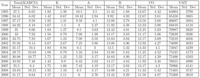
ConnDOT has average daily VMT for each year for various definitions of facility type based on urban or rural location and functional classification. Also ConnDOT has pneumatic tube and induction loop counters from which these annual average daily VMT estimates are derived. To obtain monthly VMTs, monthly expansion factors obtained from ConnDOT were used. Descriptive statistics of the response variables and VMT used in the analysis are given in Table 3.2.1.
Table 3.2.1: Descriptive Statistics of Pedestrian Crash Counts and VMT
Year Total(KABCO) K A B CO VMT
Mean Std. Dev. Mean Std. Dev. Mean Std. Dev. Mean Std. Dev. Mean Std. Dev. Mean Std. Dev.
1995 37.5 6.65 1.92 1.38 10.5 3.5 11.42 1.88 13.67 4.42 64904 3799 1996 34.41 6.02 1.42 0.67 10.42 2.94 9.92 4.93 12.67 2.61 65450 3865 1997 37.17 9.58 1.92 1.31 9.58 4.1 12.08 3.78 13.58 3.68 66687 3894 1998 34.92 8.18 1.67 1.3 8 2.37 11.92 4.38 13.33 3.98 68810 4118 1999 35 8.66 1.83 1.27 8.5 3.63 12.42 4.01 12.25 5.03 70987 3820 2000 33 7.92 1.58 0.79 7.08 1.98 13.17 3.83 11.17 5.06 72639 3936 2001 33.75 7.82 1.67 1.23 7.08 3.58 12.83 3.04 12.17 3.69 73219 4056 2002 35.92 9.14 2.67 2.67 7.25 3.86 13.08 4.06 12.92 4.27 74690 4033 2003 35.17 10.4 1.83 0.94 6.5 3 12.5 5.32 14.33 4.5 74947 4229 2004 29.75 10.63 1.08 0.79 5.33 2.84 12.08 5.82 11.25 4.52 75245 4173 2005 30.08 10.77 1.75 1.22 5.33 3.17 10.83 4.99 12.17 4.39 75490 4593 2006 33.92 7.48 1.42 0.9 6.42 2.02 14.17 4.82 11.92 3.48 76055 4990 2007 35.5 6.4 1.75 1.66 7.42 4.19 13.17 2.62 13.17 4.3 76966 4141 2008 33.83 10.21 1.92 1.16 6.5 3.17 14.08 4.21 11.33 5.42 75405 3747 2009 31.17 6.64 1.17 1.11 6 2.76 12.42 3.29 11.58 4.87 75308 3818
3.2.2
Model Framework
In this section, we model compositional data which is represented by proportions of
J = 4 different severity levels (K, A, B, CO) of monthly pedestrian crashes in Con-necticut between 1995 and 2009. We use the Box-Cox transformation together with VAR techniques, carry out the data analysis, and highlight the important findings with respect to the interpretation of the results and the estimation of the coefficients. Given crash counts in injury severity categories K, A, B, and CO, we form the propor-tions Xti by dividing the counts in each category by the total number of pedestrian
crashes, i.e,
Xti =
Cti
Ct,T otal
, (3.2.1)
whereCti represents the count of pedestrian crashes for severity category i(K, A, B,
CO) during month t (t = 1, . . . , T), where T = 180, so that Ct,T otal represents the
total count of pedestrian crashes during month t. The ALR transformation has the formYti = log(Xti/XtJ), for i= 1, . . . , g,XtJ being a reference (baseline) component
for t = 1, . . . , T, and “log” denotes the natural logarithm. Dividing by a reference (baseline) component takes care of the dimensionality problem, while taking the log-arithm is intended to transform the data to normality. In the following applications
J = 4 and g = 3. We use the Box-Cox transformation with a small adjustment d to avoid issues with logarithms; fort= 1, . . . ,180, i=“K”,“A”,“B”, andJ =“CO”, and
d= 10−5 (different values of dwere tried and did not give different results).
Yti= Xti XtJ+d λ −1 λ if λ 6= 0 log Xti XtJ +d if λ = 0 (3.2.2)
The next step is to fit a suitable multivariate model to the transformed data yt = (YtK, YtA, YtB)0 whose components are real-valued. We fit a vector autoregressive
model of order p (VAR(p)) with regressors (Reinsel, 1993):
yt=
p
X
k=1
Φkyt−k+ηut+γt+Sδ+wt, (3.2.3)
where Φk is a 3×3 AR (autoregressive) matrix of lag k, for k = 1, . . . , p; η is a
of coefficients corresponding to the time trend; S is a 3×12 parameter matrix for the seasonal part; δ is an indicator vector corresponding to the seasonal part, andwt
is a 3-dimensional vector of i.i.d. Normal(0,Σ) errors.
3.2.3
Model Estimation
The first step in the compositional analysis is to choose an appropriate value of the parameter λ in the Box-Cox transformation, as well as the order p for the VAR model. We use the Mean Absolute Error (MAE) criterion throughout the chapter for predictive validation and model selection. We calculate the within sample MAE as well as out-of-sample MAE using 6 and 12 months of holdout data using the formula. Recall that we have 4-variate counts time series data, namely number of pedestrian crashes with K, A, B and CO injury severities, for 180 months. We hold out the last L = 6 months or L = 12 months for predictive validation, and respectively use first 180−L, i.e., 174 or 168 observations for model fitting/calibration. The MAE is defined as MAE = 1 T T X i=1 |yi−ybi|, (3.2.4)
where yi denotes the ith observed value, and ybi is the ith fitted or predicted value
under the particular model.
We iterateλfrom−2 to 2 in steps of 0.1 and record the within sample MAE for all severity levels together for the best VAR(p) model for 1≤ p≤ 10; the best VAR(p) model corresponds to the fitted model with lowest Akaike Information Criterion (AIC) (Akaike, 1974). That is, we compute MAEALL based on the proportions data which
we obtain by transforming back the Box-Cox transformed compositions:
MAEALL = MAEK+ MAEA+ MAEB+ MAECO (3.2.5)
The smallest MAEALL is 0.2189 with VAR of orderp= 1 (the lowest AIC is−6.5796). We use the function VAR in the R package vars for the VAR(p) model fitting and the function bxcx in the R package FitAR for doing the Box-Cox transformation.
The fitted model for the transformed compositions corresponding to injury severity level K follows from (3.2.3) and is written as
b
Yt,K =φb11,KYt−1,K +φb12,AYt−1,A+φb13,BYt−1,B+ηbKut+bγKt+Sb
0
Kδ, (3.2.6)
where (φb11,K,φb12,A,φb13,B) is the first row of estimated matrix Φ and SbK is the first
row of S;bγK and bηK are respectively the first components of the estimated vectorsγ
and η. Partial output for the fitted coefficients in (3.2.6) is shown in the top portion of Table 3.2.2, in rows 1−5. Note that the seasonal coefficients are suppressed from the output for brevity. March, July, August and November coefficients have the smallest p-values, which are respectively 0.0708, 0.1171, 0.0294 and 0.0871; and the corresponding estimated values of the seasonal effects, with standard errors shown in brackets, are respectively −0.1538(0.0845), −0.1325(0.0841), −0.1884(0.0856), and
−0.1458(0.0847).
The fitted model for the transformed compositions corresponding to injury severity level A follows from (3.2.3) and is written as
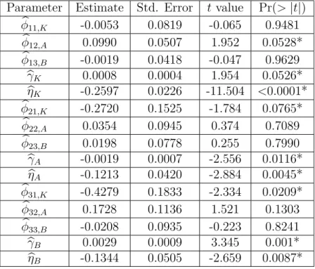
Table 3.2.2: Estimated Coefficients for level K, A and B Transformed Compositions
(* denotes significantp-values with significance levelα= 0.1)
Parameter Estimate Std. Error t value Pr(>|t|)
b φ11,K -0.0053 0.0819 -0.065 0.9481 b φ12,A 0.0990 0.0507 1.952 0.0528* b φ13,B -0.0019 0.0418 -0.047 0.9629 b γK 0.0008 0.0004 1.954 0.0526* b ηK -0.2597 0.0226 -11.504 <0.0001* b φ21,K -0.2720 0.1525 -1.784 0.0765* b φ22,A 0.0354 0.0945 0.374 0.7089 b φ23,B 0.0198 0.0778 0.255 0.7990 b γA -0.0019 0.0007 -2.556 0.0116* b ηA -0.1213 0.0420 -2.884 0.0045* b φ31,K -0.4279 0.1833 -2.334 0.0209* b φ32,A 0.1728 0.1136 1.521 0.1303 b φ33,B -0.0208 0.0935 -0.223 0.8241 b γB 0.0029 0.0009 3.345 0.001* b ηB -0.1344 0.0505 -2.659 0.0087* b Yt,A=φb21,KYt−1,K+φb22,AYt−1,A+φb23,BYt−1,B+ηbAut+bγAt+Sb 0 Aδ, (3.2.7)
where (φb21,K,φb22,A,φb23,B) is the second row of estimated matrix Φ, SbA is the second
row of S; bγA and ηbA are the second components of the estimated vectors γ and η
respectively. Partial output for the fitted coefficients in (3.2.7) is shown in the middle portion of Table 3.2.2, in rows 6−10. Again, results on the seasonal effects are not shown. Only January has a relatively small p-value of 0.1118, with corresponding estimated value (standard error) of 0.2566 (0.1604).
level B follows from (3.2.3) and is written as b Yt,B =φb31,KYt−1,K +φb32,AYt−1,A+φb33,BYt−1,B + b ηBut+bγBt+Sb 0 Bδ, (3.2.8)
where (φb31,K,φb32,A,φb33,B) is the third row of estimated matrix Φ, SbB is the third
row of S; γbB and ηbB are the third components of the estimated vectors γ and η
respectively. Partial output for the fitted coefficients in (3.2.8) is shown in the bot-tom portion of Table 3.2.2, in rows 11−15. The seasonal coefficients for February and November have the smallest p-values of 0.132 and 0.1057 with corresponding estimated values (standard errors) of 0.2901 (0.1916) and −0.3086 (0.1896).
The estimated covariance matrix of residuals from (3.2.3) is
0.0441 0.0155 0.0176 0.0155 0.153 0.0908 0.0176 0.0908 0.221
The matrix of residuals is an estimate of the covariance matrix Σ of the error term wt in equation (3.2.3). Small off-diagonal values indicate almost no correlation
between elements of vector yt. The values on the diagonal represent the estimated
variance of proportions K, A and B over the baseline CO transformed by (3.2.2). The fitted model indicates that the proportion of B level crashes over the proportion of CO level crashes has the largest residual variance, followed by the proportion of A level and K level crashes over the CO level.
We ran standard diagnostics procedures to assess out model fit. Cross-correlation plots of residuals and the adjusted multivariate Portmanteau test (Hosking, 1980) indicated that the fitted models were adequate. Normal Q-Q plots of the residuals
indicated that the assumption of normality is reasonable.
3.2.4
Discussion of Results
We have modeled the data Yti which is proportional to the ratio of proportions of
crashes of K, A or B levels over the CO level. Thus, a decrease in Yti is desirable
in terms of transportation safety as it indicates a smaller proportion of crashes for more severe injury levels over the CO (the least severe) level. All three estimates of the elements of the vector γ are significant, which suggests a strong indication of a time trend for all three components. There is a substantial increase in the proportion of B level crashes over time, with bγB = 0.0029 (0.0009) with respect to the baseline
CO level. Coefficients also indicate a somewhat smaller decrease of severity A level crashes with bγA = −0.0019 (0.0007), and just a slight increase of severity K level
crashes with bγK = 0.0008 (0.0004), all relative to the baseline CO level. All three
estimated components of the η vector are significant and negative, which indicates that an increase in VMT results in a decrease in the proportions of all other crash levels (K, A and B) with respect to the baseline CO level. All significant seasonal coefficients are negative except in January for A level crashes and in February for B level crashes, which indicates an increase in those two months for A and B severity level crashes over the baseline CO level. Estimated entries of theΦmatrix represent the serial correlation between transformed compositions at one time lag.
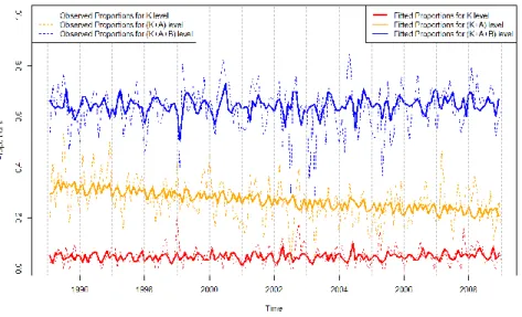
To visualize results from the compositional time series analysis, we show stacked plots for different injury severity proportions of pedestrian crashes in Figure 3.2.1. Proportions of K, A, B and CO injury severity levels are obtained from the fitted model (3.2.3) using the inverse transformation from (3.2.2). The solid lines at the
bottom, middle, and top of the plot denote respectively the fitted proportions of level K, level (K+A) and level (K+A+B) crashes. The dotted lines at the bottom, middle and top denote respectively the corresponding observed proportions at levels K, (K+A) and (K+A+B). The stacked plot is done to avoid the overlapping of fitted and observed proportions and is more meaningful as a graphical representation.
Figure 3.2.1: Stacked Plot of Fitted Proportions of Compositional Model
From Figure 3.2.1, we note that an overall model fit to the data is satisfactory and underline the conclusions we had made based on the estimated coefficients. We have managed to get rid of unwanted noise and extract a clear behavior of the compositional time series data. We have also verified our conclusions about time trend in the data. There is a noticeable significant decrease in the proportion of severity level A crashes over time, with an increase in pedestrian crashes with severity level B, while K and CO stay approximately on the same level over this time period. In other words, there
is an apparent migration of crashes from the higher severity level A to lower severity level B, suggesting that pedestrian injury severity is on average decreasing over time.
3.3
Dynamic and Static Modeling of Pedestrian
Crash Counts
In this section, we describe the dynamic and the static modeling of the total pedestrian crash counts, aggregated over all injury severity levels. Hu et al. (2012) described the estimation of such models and the predictions for all vehicle crashes. We extend this analysis to the pedestrian crashes.
We fit a dynamic model for the total pedestrian crash countsCt,T otalfor notational
simplicity, we write this simply as Ct in this section. The observation equation is
written either using a conditional Poisson distribution in (3.3.1a) or a conditional negative binomial distribution in (3.3.1b):
Ct|λt ∼ Poisson(λt) (3.3.1a)
Ct|λt, k ∼ NegBin(λt, k), (3.3.1b)
where λt is the mean and k is the shape parameter; we model the latent variable λt
as
λt = αt×V
η
t ×exp(St)
or
Define βt= log(αt). The trendβt and seasonal components St are modeled as
βt = ρ×βt−1+wt t= 2, . . . ,180 (3.3.3a)
St = −(St−1+· · ·+St−11) +wt t= 12, . . . ,180, (3.3.3b)
where βt is the dynamic intercept coefficient; Vt represents VMT; η represents the
static coefficient for log(VMT); ρrepresents the coefficient in the autoregressive pro-cess (AR(1) process); and St is the seasonal component to explain periodic behavior
of period 12; wt is i.i.d. Normal(0, a2); vt is i.i.d. Normal(0, b2). We refer to this
model as a Dynamic Generalized Linear Model (DGLM). The response variable is a count variable and since its conditional distribution is non-Gaussian, the standard Kalman Filter algorithm cannot be used to obtain the posterior distributions of the unknown parameters, which do not have closed forms. Gamerman (1998) suggested a fully Bayesian approach for DGLMs using Markov chain Monte Carlo techniques This approach can be computationally intensive, and we therefore implement approximate Bayesian inference using INLA approach proposed by Rue et al. (2009). The dynamic model described above enables us to fit and predict total pedestrian crash counts. We implement this method using the R package INLA available through webpage www.r-inla.org. Ruiz-C´ardenas et al. (2012) give an excellent guidance for fitting dynamic models using the R-INLA package, which includes numerous simulated and real data examples.
The static model is widely used, and is defined via (3.3.1a) or (3.3.1b), where now
λt = α×Vtη ×exp(γ×t+s
0×
δ) or
log(λt) = log(α) +η×log(Vt) +γ×t+s0 ×δ (3.3.4)
Here, log(α) is static intercept coefficient; η represents the static coefficient for log(VMT); γ represents time trend coefficients; s0 is a 1×11 parameter vector cor-responding to the seasonal part; δ is 11×1 an indicator vector corresponding to the seasonal part and other terms are defined earlier under the dynamic model.
We fitted the negative binomial model and the Poisson model for Ct for both the
static and dynamic models. The AIC criterion for the negative binomial static model was 1125.4 which was slightly larger than the AIC value of 1125.3 for the Poisson distribution static model (the overdispersion coefficient was also not significant). The Deviance Information Criterion (DIC) value was 1175.13 for the negative binomial dynamic model, which was higher than the value of 1121.3 in the Poisson case. The smaller values of AIC and DIC indicate the better models, therefore we present re-sults from the Poisson static and dynamic models. In the static model described by (3.3.1a) and (3.3.4), the interceptα(which also represents the coefficient for January in the model with seasonal indicator variables), as well as the seasonal coefficients from February through August are significant. Estimated values (standard errors) for α, and corresponding seasonal coefficients are 7.4453 (2.4860), −0.2598 (0.0687),
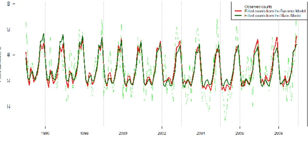
−0.3108 (0.0765), −0.2827 (0.0915), −0.2960 (0.1120), −0.3817 (0.1199), −0.3885 (0.1187), −0.2986 (0.1192), −0.1745 (0.1038). Estimated coefficients η and γ (effect of VMT and time) appear to be not significant. Figure 3.3.1 shows a plot of observed
total pedestrian crash counts, together with fitted values from the Poisson static and dynamic models. From the plot, we can conclude that both models fit the observed data well, and they manage to capture the seasonal part for almost all time periods. However, there are some differences in the fit of static and dynamic models between 2004 and 2006 years, which we will explain later.
Figure 3.3.1: Pedestrian Crash Counts with the Model Fits
The dynamic model in (3.3.1a)-(3.3.3b) can also be used for modeling crash counts
Cti by injury severity levels. In order to assess differences in fitted values of static
and dynamic models we need to explain the differences in the models itself. The main difference is coming from the way to model time trend coefficient. In the static model it stays the same during all time period, but for the dynamic model we allow to have dynamic intercept (represents time trend coefficient) to vary over the time
which is more natural behavior in real life situations. Figure 3.3.2 gives a plot of estimated dynamic coefficient αt from the model (3.3.1a)-(3.3.3b) (according to the
Bayesian model, it is posterior mean for intercept) for total counts as well as for level A severity injury crashes. The dynamic intercepts for K, B and CO injury severity crash levels have very slight changes in dynamic behavior, staying at the same level (αt ≈1) throughout the observational period and are omitted in the Figure 3.3.2 to
avoid the overlaps.
Figure 3.3.2: Temporal Behavior ofαt
From Figure 3.3.2, we observe an overall decrease in the total number of pedestrian crashes from 1995 to April 2005, then, an increase until May 2007, and then leveling off until the end of the time period. That is exactly the same period where the dynamic model differs from the static model. The reason is that the static model failed to
catch the dynamic behavior of the trend. We recall that the dynamic models for different injury severity crash counts account for the effect of VMT, seasonal period, and random variation in the counts due to the Poisson distribution. We observe that the main reason for the increase in total counts is an increase in the counts of level A injury severity pedestrian crashes, while counts of the other injury severity crashes do not show changes in the αt values. In other words the results from the dynamic
model show no temporal effects for K, B, or CO severity levels, thus a reduction in level A will result in fewer total crashes.
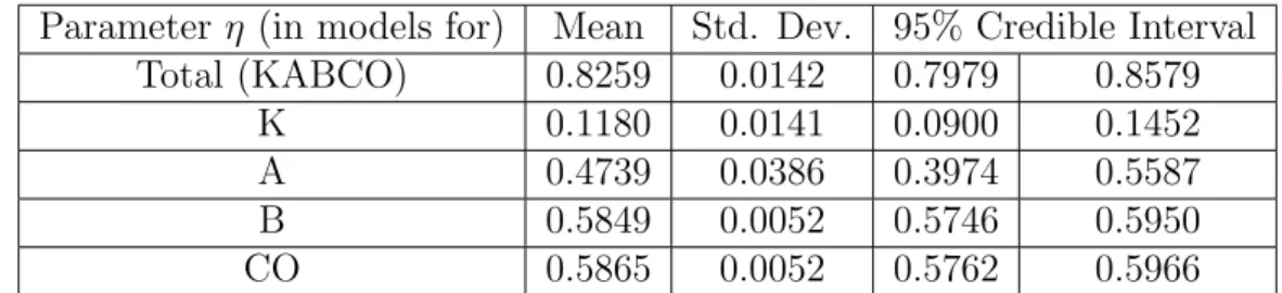
From Table 3.3.1, we conclude that an increase in VMT results in an increase in total pedestrian crashes as well as in all injury severity level crashes. The effect of the increase is the largest for the CO level crashes followed by B, A and K levels. This result coincides with the finding from the compositional model where the negative sign for VMT suggests the slower increase in K, A and B level crashes than in CO level crashes (the baseline).
Table 3.3.1: Estimated static coefficients for the VMT effect in the dynamic models Parameter η (in models for) Mean Std. Dev. 95% Credible Interval
Total (KABCO) 0.8259 0.0142 0.7979 0.8579 K 0.1180 0.0141 0.0900 0.1452 A 0.4739 0.0386 0.3974 0.5587 B 0.5849 0.0052 0.5746 0.5950 CO 0.5865 0.0052 0.5762 0.5966
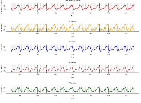
The estimated seasonal components are shown in Figure 3.3.3. The total (KABCO) crashes have the lowest peak in March, which migrates to February after 2001. We can notice the intermediate peak around May, followed by an increase in crashes until December. Overall, the seasonal effect is negative from February until August, and stays positive for the remaining months. The seasonal effect for K level crashes is
neg-ative from February until July and in September with the lowest values during March and July and the largest value in December. The A level crashes are influenced by the negative seasonal effect during January-August months. Months January through April and June through September have negative effect on B level crashes. Similar to the total crashes, February through August have negative effects on the CO level crashes.
3.4
Predictions of Crash counts by Injury Severity
Levels
We combine the approaches described in Sections 3.2 and 3.3 in order to construct fits/predictions for the pedestrian crash counts by injury severity levels. We also compare the predictions obtained by using the static or the dynamic models for fitting the total pedestrian crashes. For the fitting portion of the data, we use 168 observations, holding out the last 12 observations for the forecast evaluation. We evaluate 6 month and 12 month ahead predictions.
We obtain fitted or predicted compositions Ybti from the compositional model
de-scribed in Section 3.2; we convert these to fitted/predicted proportionsXbtivia (3.2.2),
and then use (3.2.1) to convert to the fitted/predicted counts at different severity lev-els, i.e.,
b
Cti=Xbti×Cbt,T otal
Here,Cbtirepresents the fitted counts of pedestrian crashes for severity leveli(K,A,B,CO)
during montht(t= 1, . . . ,180);Cbt,T otalrepresents the fitted total counts of pedestrian
crashes by static or dynamic models during montht; Xbti represents the fitted
propor-tions of pedestrian crashes by compositional model for severity level i (K,A,B,CO) during month t (t= 1, . . . ,180).
Table 3.4.1 shows a comparison between different models in terms of the Mean Absolute Error criterion (MAE) by comparing Cti with Cbti using:
MAEi = 1 T T X t=1 |Cti−Cbti|
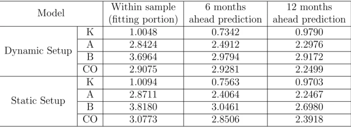
Table 3.4.1: MAE comparison
Model Within sample 6 months 12 months (fitting portion) ahead prediction ahead prediction
Dynamic Setup K 1.0048 0.7342 0.9790 A 2.8424 2.4912 2.2976 B 3.6964 2.9794 2.9172 CO 2.9075 2.9281 2.2499 Static Setup K 1.0094 0.7563 0.9703 A 2.8711 2.4064 2.2467 B 3.8180 3.0461 2.6980 CO 3.0773 2.8506 2.3918
The Dynamic Setup and the Static Setup respectively refer to predicting the total crash counts via the dynamic model (3.3.1a)-(3.3.3b), or the static model (3.3.1a) and (3.3.4), while Xbti follows from the compositional model in both cases. From Table
3.4.1, we see that the dynamic setup has lower MAE values for all within sample fits, but the static setup gives better out-of-sample predictions for 6 and 12 month holdout data.
3.5
Discussion and Conclusions
The main goal of this analysis was to explore how the proportions of different injury severity levels may be changing over time relative to one another, and to assess how pedestrian safety has changed over the observational time period. Through our sta-tistical analysis, we were able to filter out the observational noise and estimate the temporal behavior of pedestrian crashes. The result of the compositional time series analysis revealed a substantial decrease in the proportions of pedestrian crashes in in-jury severity level A, and an increase in the level B proportions. The magnitude of the proportions of the K level showed relatively no change over the observational period
on urban roads in Connecticut. Moreover, we found indications of an increase in the proportions of levels A and B over the baseline (CO) during January and February with respective positive coefficients (standard errors) given by 0.2566 (0.1604) and 0.2901 (0.1916). We compared two different approaches for fitting/predicting pedes-trian crash counts by injury severity level, viz., the Dynamic Setup and the Static Setup. The Dynamic Setup combines the fitted/predicted monthly proportions from the compositional model (3.2.1)-(3.2.3) and the fitted/predicted monthly total crash counts from the dynamic model (3.3.1a)-(3.3.3b). The Static Setup combines the fitted predicted monthly proportions from the compositional model (from Section 3.2) and the fitted predicted monthly total crash counts from the static model (from Section 3.3).
Additionally, the dynamic modeling for the pedestrian crash counts Cbti enables
us to investigate the temporal behavior of αt for the different severity levels. We
uncovered a decreasing trend in all pedestrian crash counts before April 2005, followed by a noticeable increase after that which lasted until May 2007, and then a flattening out until the end of the fitting period. This behavior appears to be largely due to changes in the severity level A pedestrian crashes.
To summarize, we conclude based on our analysis that the overall pedestrian safety on urban roads in Connecticut is increasing, because we discovered a shift into the less severe injury level (from level A to level B). Moreover, the behavior of total pedestrian crash counts appears to mirror the behavior of the level A crash counts. We suggest that more attention has to be focused on the pedestrian safety in the months of January and February, as we observed an increasing proportion of the A and B level crashes over the baseline CO level for these two months. Our analysis is essential for the segment/intersection study where the road side characteristics could
be controlled. With a rareness of pedestrian crashes it is impossible to investigate monthly temporal effects with an individual segment/intersection level data, thus the time dependence should be derived from the aggregated level data and then incorporated into segment/intersection study for example as a sampling strategy. Moreover dynamic models can uncover trends that can be used in conjunction with known application of pedestrian safety interventions on the statewide level to test their effectiveness. Our approach has also uncovered seasonal effects which are also useful for identifying at which times of year pedestrian safety is a consistently more serious issue. This can help with identifying interventions that would be appropriate for the pedestrian safety issues at those times of year. Overall the dynamic models can be used to monitor trends in pedestrian safety and can help to react in a timely manner to situations on the roads.
Hierarchical Dynamic Models for
Multivariate Times Series of
Counts
In this chapter, we describe a hierarchical multivariate dynamic model (HMDM), with a multivariate Poisson distribution (MVP) as the sampling distribution for the response vector time series of counts, and incorporating covariates that may vary over location and/or time. The use of the MVP distribution enables us to model associations between the components of the count response vector, while the dynamic framework allows us to model the temporal behavior. The hierarchical structure enables us to capture the location (or subject) specific effects over time.
The format of this chapter follows. Section 4.1 gives a description of the ecolog-ical application, including a description of the data. Section 4.2 reviews the MVP distribution and describes fast computation of its probability mass function (pmf). Section 4.3 describes the HMDM model and gives details of the Bayesian inference.
Section 4.4 discusses model selection and