& % CONSTRAINT-BASED MINING OF FREQUENT
ARRANGEMENTS OF TEMPORAL INTERVALS
PANAGIOTIS PAPAPETROU
Thesis submitted in partial fulfillment of the requirements for the degree of
Master of Arts
BOSTON
UNIVERSITY
GRADUATE SCHOOL OF ARTS AND SCIENCES
Thesis
CONSTRAINT-BASED MINING OF FREQUENT ARRANGEMENTS OF TEMPORAL INTERVALS
by
PANAGIOTIS PAPAPETROU
B.Sc., University of Ioannina, Greece, 2003
Submitted in partial fulfillment of the requirements for the degree of
Master of Arts 2007
First Reader
George Kollios, PhD
Assistant Professor of Computer Science
Second Reader
Stan Sclaroff, PhD
and not everything that counts can be counted;
Albert Einstein (1879-1955)
ARRANGEMENTS OF TEMPORAL INTERVALS PANAGIOTIS PAPAPETROU
ABSTRACT
The problem of discovering frequent arrangements of temporal intervals is studied. It is assumed that the database consists of sequences of events, where an event occurs dur-ing a time-interval. The goal is to mine temporal arrangements of event intervals that appear frequently in the database. The motivation of this work is the observation that in practice most events are not instantaneous but occur over a period of time and different events may occur concurrently. Thus, there are many practical applications that require mining such temporal correlations between intervals including the linguistic analysis of an-notated data from American Sign Language as well as network and biological data. Two efficient methods to find frequent arrangements of temporal intervals are described; the first one is tree-based and uses depth first search to mine the set of frequent arrangements, whereas the second one is prefix-based. The above methods apply efficient pruning tech-niques that include a set of constraints consisting of regular expressions and gap constraints that add user-controlled focus into the mining process. Moreover, based on the extracted patterns a standard method for mining association rules is employed that applies differ-ent interestingness measures to evaluate the significance of the discovered patterns and rules. The performance of the proposed algorithms is evaluated and compared with other approaches on real (American Sign Language annotations and network data) and large synthetic datasets.
1 Introduction 1
2 Background 6
2.1 Event Interval Temporal Relations . . . 6
2.2 Robustness and Ambiguity Issues . . . 8
2.3 Arrangements and Arrangement Rules . . . 9
2.4 Interestingness Measures . . . 11
2.4.1 Anti-monotone Interestingness Measures . . . 13
2.4.2 Non Anti-monotone Interestingness Measures . . . 13
2.5 Temporal and Structural Constraints . . . 14
2.6 Problem Formulation . . . 16
3 Related Work 18 3.1 Sequential Pattern Mining Algorithms . . . 18
3.1.1 Apriori-based Algorithms . . . 18
3.1.2 Tree-based Algorithms . . . 19
3.1.3 Lattice-based Algorithms . . . 20
3.1.4 Algorithms with Regular Expression Constraints . . . 21
3.1.5 Prefix-based Algorithms . . . 22
3.1.6 Algorithms for Mining Closed Sequential Patterns . . . 23
3.2 Temporal Mining and Association Rules . . . 23
3.3 Interestingness Measures . . . 26
4.2 BFS-based Approach . . . 30
4.3 DFS-based Approach . . . 33
4.4 Hybrid DFS-based Approach . . . 34
4.5 A Prefix-based Approach . . . 35
4.6 Applying Other Interestingness Measures . . . 36
4.6.1 Handling Non Anti-monotone Interestingness Measures . . . 37
4.6.2 Handling Anti-monotone Interestingness Measures . . . 39
5 Experimental Evaluation 43 5.1 Experimental Setup . . . 43
5.1.1 Experiments on Real Data . . . 44
5.1.2 Experiments on Synthetic Data . . . 50
6 Conclusions 54
References 56
1·1 An ASL example. . . . 2
1·2 A network example. . . . 4
2·1 Basic relations between two event-intervals: (a) Meet, (b) Match, (c) Over-lap, (d) Contain, (e) Left-Contain, (f) Right-Contain, (g) Follow.. . . 7
2·2 Lack of Robustness in Allen’s Relations. . . . 8
2·3 An Example of an e-sequence. . . . 10
2·4 (a) S0 can be expressed with four operands and (b)S00 cannot. . . . . 15
4·1 An e-sequence database D.. . . 29
4·2 An arrangement enumeration tree. . . . 30
4·3 ISId-Lists for items A and B. . . . 31
4·4 An Example of a Projection.. . . 36
4·5 An Example of an e-sequence database of two records and a projection that does not work. . . . 37
4·6 The set of frequent2 and3-arrangements. . . . 42
5·1 Some Frequent Patterns of Datasets1, 2 and 3.. . . 45
5·2 Results on Real Datasets: (a) ASL Dataset1: |S|: 73,|A|: 52,|E|: 400.; (b) ASL Dataset 2: |S|: 68, |A|: 26, |E|: 400.; (c) ASL Dataset3: |S|: 884,|A|: 102, |E|: 400.; (d) Network Dataset: |S|: 960,|A|: 100,|E|: 200 (where|S| denotes the size of the dataset, |A|the average sequence size), and |E|the number of distinct items in the dataset. . . . 50
patterns of medium density.; (b) Dataset 2: |S|: 1000, |A|: 20, |E|: 600, sparse frequent patterns.; (c) Dataset 3: |S|: 1000,|A|: 50, |E|: 800, dense frequent pat-terns.;(d) Dataset4: |S|: 2000,|A|: 10,|E|: 400, frequent patterns of medium
den-sity.;(e) Dataset 5: |S|: 2000,|A|: 20,|E|: 400, frequent patterns of medium
den-sity.;(f) Dataset6: |S|: 5000,|A|: 20,|E|: 400, dense frequent patterns.;(g) Dataset
7: |S|: 5000, |A|: 50,|E|: 400, dense frequent patterns.;(h) Dataset8: |S|: 10000,
|A|: 100,|E|: 800, dense frequent patterns. . . . 53
ASL . . . American Sign Language
DNA . . . DeoxyriboNucleic Acid
ISIdList . . . Interval Sequence Id List
BFS . . . Breadth First Search
DFS . . . Depth First Search
ODFlow . . . Origin Destination Flow
IP . . . Internet Protocol
Introduction
Sequential pattern mining has received particular attention in the last decade (Agrawal and Srikant, 1994; Agrawal and Srikant, 1995; Ayres et al., 2002; Bayardo, 1998; Zaki, 2001; Fei et al., 2001; Pei et al., 2002; Han et al., 2000a; Seno and Karypis, 2002; Yan et al., 2003; Leleu et al., 2003; Han et al., 2000b; Wang and Han, 2004). The objective is to extract patterns from a set of sequences of instantaneous events which satisfy some user-specified constraints. These constraints can vary from just a support threshold, that defines frequency, to a set of gap, window (Zaki, 2000; Srikant and Agrawal, 1996), or regular expression constraints (Garofalakis et al., 1999), that push more user-controlled focus into the mining process. Despite advances in this area, nearly all proposed algo-rithms concentrate on the case where events occur at single time instants. However, in many applications events are not instantaneous; they instead occur over a time interval. Furthermore, since different temporal events may occur concurrently, it would be useful to extract frequent temporal patterns of these events. In this paper the goal is to develop methods that discover temporal arrangements of correlated event intervals which occur frequently in a database.
There are many applications that require mining such temporal relations. One po-tential application is for analysis of the multiple gestures that occur, in parallel, on the hands and on the face and upper body, to express linguistic information. In signed lan-guages, lexical information is expressed primarily through movements of the hands and arms, whereas critical grammatical information is expressed non-manually, through such
> Who drove the car, who?
(Lowered eyebrows)
(Wh-Question) (Wh -Word)
time
(Rapid head shake) (Rapid head shake) (Wh -Word) (Lowered eyebrows)
Figure 1·1: An ASL example.
behaviors as raised or lowered eyebrows, modifications in eye aperture or gaze, repeated head gestures (nods, shakes) or head tilt, as well as expressions of the nose or mouth. For example, the canonical marking of a wh-question (a question containing a word such as ’who’, ’what’, ’when’, ’where’, or ’why’) includes lowered brows slightly squinted eyes oc-curring over a predictable domain (either the question sign or the whole clause constituting the question), and there is frequently a slight rapid head-shake co-occurring with the wh-phrase (Neidle and Lee, 2006). Although much is known about the linguistic significance of certain non-manual markings carrying critical syntactic information, there are others whose functions remain to be studied and more fully understood. Pattern detection could ultimately contribute to discovery of the significance of some of these non-manual behav-iors. The annotated ASL corpus used for this research was produced by linguists as part of the American Sign Language Linguistic Research Project ((Neidle et al., 2000; Neidle, 2003; Neidle and Lee, 2006)) using SignStream(TM) ((Neidle et al., 2001; Neidle, 2002a)). The annotations identify start and end times for: the manual ASL signs (represented by English-based glosses), part of speech for those signs, plus grammatical interpretive labels indicating clusters of non-manual expressions that serve to mark particular syntactic func-tions (such as wh-quesfunc-tions, negation, etc.) as well as the gestures themselves (e.g., raised eyebrows, wrinkled nose, rapid head shake). See ((Neidle, 2002b)) for further information about the annotation conventions that were used.
Another application is in network monitoring, where the goal is to analyze packet
communicating with each other via two routers. In this case an event label is the source and destination IP and the event interval corresponds to the duration of the communication between the two machines. Multiple types of events occurring over certain time periods can be stored in a log, and the goal is to detect general temporal relations of these events that with high probability would describe regular patterns in the network, that could be used for prediction and intrusion detection.
Moreover, interval-based events can be identified in the human gene. More specifically, DNA is a sequence of items (nucleotides) defined over a four-letter alphabet, i.e. Σ =
{A, C, G, T}. Regions of high occurrence of a nucleotide or combination of nucleotides,
known as poly-regions, can be defined over DNA. The detection of frequently overlapping
poly-regions could lead the biologists to a variety of useful observations concerning the evolution of different genes and their contribution to protein construction. To the best of our knowledge, the first general approach to mine frequent arrangements of poly-regions in DNA is introduced in (Papapetrou et al., 2006).
Most existing sequential pattern mining methods are hampered by the fact that they can only handle instantaneous events, not event intervals. Nonetheless, such algorithms could be retrofitted for the purpose, via converting a database of event intervals to a transactional database, by considering only the start and end points of every event interval. An existing sequential pattern mining algorithm could be applied to the converted database, and the extracted patterns could be post-processed to produce the desired set of frequent
arrangements. However, an arrangement ofkintervals corresponds to a sequence of length
2k. Hence, this approach will produce up to 22k different sequential patterns. Moreover,
post-processing will also be costly, since the extracted patterns consist of event start and end points, and for each event interval all the relations with the other event intervals must be determined. Therefore, it is essential to develop interval-based algorithms that can efficiently mine frequent patterns and rules from interval-based data.
The main contributions in this paper include:
Router 1 Router 2 IPs IPs A B (D, C) (D, B) (A, B) D C time
Figure 1·2: A network example.
tolerant and through the use of constraints eliminates the ambiguity of Allen’s defi-nitions (Allen and Ferguson, 1994),
• a formal definition for the problems of mining frequent temporal arrangements and
arrangement rules of event intervals in an event interval database using temporal and structural constraints,
• a prefix-based approach and an efficient algorithm for mining frequent arrangements
of temporally correlated events using depth first search in an enumeration tree of temporal arrangements,
• a further improvement of the mining process with the incorporation of temporal and
structural constraints,
• an efficient algorithm for mining arrangement rules from the extracted patterns based
on user-specified interestingness measures and constraints, and
• an extensive experimental evaluation of these techniques and a comparison with a
standard sequential pattern mining method, SPAM (Ayres et al., 2002), using both real and synthetic data sets,
The remainder of this thesis is organized as follows: Chapter 3 presents the related work on sequential pattern mining, interval mining and temporal mining. Also it gives a brief
overview of the existing interestingness measures for association rules. Chapter 2 provides the problem formulation along with the appropriate definitions and background. Chapter 4 gives an extensive description of two tree-based approaches and a prefix-based approach for mining frequent arrangements of temporally correlated event intervals. Also, in the
same Chapter, an efficient algorithm for extracting the set of top k arrangement rules is
described. Chapter 5 describes the experimental evaluation, and Chapter 6 concludes the thesis, providing directions for future research.
Background
Some basic definitions on temporal logic are presented, followed by a sufficient background on interestingness measures for association rules. Finally, the problems of constraint-based mining of frequent arrangements of temporal intervals and constraint-based mining of the
topK interesting association rules from a database of interval-based events are formulated.
2.1 Event Interval Temporal Relations
Seven types of temporal relations between two event intervals are considered. Using these relations, general arrangements can be defined. However, the methods presented in this thesis are not limited to these relations and can be easily extended to include more types of temporal relations, as the ones described by Allen in (Allen and Ferguson, 1994) and also later on in (Freksa, 1992).
Consider two event-intervals A and B. Furthermore, assume that the user specifies a
threshold²used to define more flexible matchings between two time instants. The following
relations are studied (see also Figure 2·1):
• Meet(A, B): In this case, B follows A, with B starting at the time A terminates,
i.e. te(A) =ts(B)±². This case is denoted asA∼B and we say thatA meets B.
• Match(A, B): In this case,Aand B are parallel, beginning and ending at the same
time, i.e. ts(A) =ts(B)±²andte(A) =te(B)±². This case is denoted asA||B and
we say that A matches B.
A[tstart, tend] B[tstart, tend] (a) Meet of A and B
A[tstart, tend] B[tstart, tend]
(d)
A[tstart, tend] B[tstart, tend] (g)
Contain of A and B
Follow of A and B
+/- e
A[tstart, tend] B[tstart, tend] (e) Left Contain of A and B
A[tstart, tend]
B[tstart, tend]
(f) Right Contain of A and B
+/- e +/- e
A[tstart, tend] B[tstart, tend]
(c) Overlap of A and B
A[tstart, tend]
B[tstart, tend]
(b) Match of A and B
+/- e +/- e
Figure 2·1: Basic relations between two event-intervals: (a) Meet, (b) Match, (c) Overlap, (d) Contain, (e) Left-Contain, (f ) Right-Contain, (g) Follow.
• Overlap(A, B): In this case, the start time of B occurs after the start time of A,
and A terminates before B, i.e. ts(A) < ts(B), te(A) < te(B) and ts(B) < te(A).
This case is denoted asA|B and we say thatA overlaps B.
• Contain(A, B): In this case, the start time ofB follows the start time ofAand the
termination of A occurs after the termination ofB, i.e. ts(A) < ts(B) and te(A) >
te(B). This case is denoted as A > Band we say that A contains B.
• Left-Contain(A, B): In this case,AandB start at the same time andAterminates
after B, i.e. ts(A) = ts(B)±² and te(A)> te(B). This case is denoted as A |> B
and we say that A lef t-contains B.
• Right-Contain(A, B): In this case, A and B end at the same time and the start
time ofA precedes that ofB, i.e. ts(A)< ts(B)and te(A) =te(B) ±². This case is
denoted as A >|B and we say thatA right-contains B.
• Follow(A, B): In this case, B occurs after A terminates, i.e. te(A) < ts(B). This
A B (a) Meet or Overlap?
A
B (d) Match or Contain?
A
B
(e) Left Contain or Contain?
A
B (f) Right Contain or Contain?
A
B (c) Match or Overlap?
A B
(b) Meet or Follow?
Figure 2·2: Lack of Robustness in Allen’s Relations.
2.2 Robustness and Ambiguity Issues
Most existing interval-based mining algorithms use Allen’s approach (Allen and Ferguson, 1994) to describe relations between event intervals. Because of the limit in the accuracy of demarcating the temporary boundaries of events, there can be variability in these bound-aries. Unfortunately, Allen’s relations are hampered by the fact that they cannot capture this variability, thus they are not robust and can be ambiguous. This issue has also been
noted in (Moerchen, 2006) and is illustrated in Figure 2·2. Consider, for instance, the case
where the actual relation between two event intervals is meet, but due to noise it appears
asoverlapas shown in Figures 2·2(a) and 2·2(b). Similarly, an actualmatch could appear
as overlap (Figure 2·2(c)) or contain (Figure 2·2(d)), and also, a lef t or right-contain
could show up ascontain(Figures 2·2(e), 2·2(f)). Such errors can occur due to noisy data
and may have a negative influence on the extracted patterns.
The aforementioned deficiency in Allen’s relations is eliminated in our definitions by
the use of an ² threshold that makes Allen’s definitions more robust and noise tolerant.
Two observations can be made regarding ². Notice that the meet relation is a subset of
the follow relation. To prevent any ambiguity, it is assumed that if two event intervals
are within a user-defined ² threshold, then their relation is meet, otherwise it is follow.
Similarly, left-contain and right-contain are subsets of contain and a clear distinction is
achieved again through the ² threshold. Thus, the use of ² in the meet, left-contain and
right-contain relations can efficiently handle “noisy” intervals.
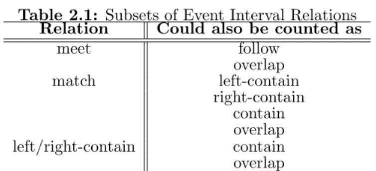
Table 2.1: Subsets of Event Interval Relations
Relation Could also be counted as
meet follow overlap match left-contain right-contain contain overlap left/right-contain contain overlap
mutually exclusive. Table 2.1 shows how these relations cannot be mutually exclusive. For
example, a match could also be counted as a left-contain, right-contain, contain and/or
overlap. Also, a left-contain or right-contain could be counted as a contain or anoverlap
as well. Finally, a meetcould also be counted as afollow oroverlap. Thus, depending on
the application, a user might desire to: (1) collapse some relations, e.g. countleft-contain
and right-contain as contain, or count each meet as follow, etc., (2) count them multiple
times, e.g. each overlap is also counted as left-contain and right-contain, or each match is
also counted ascontain, or eachmeet is also counted as follow, etc.
Thus, the user has flexibility with respect to which of these options get chosen and clearly it would be application specific. The user is given the aforementioned flexibility through the implementation of a graphical user interface, which is relatively straightfor-ward.
2.3 Arrangements and Arrangement Rules
Let E = {E1, E2, ..., Em} be an ordered set of event intervals, called event interval
se-quence or e-sequence. Each Ei is a triple (ei, tistart, tiend), where ei is an event
la-bel, ti
start is the event start time and tiend is the end time. The events are ordered
by the start time. If an occurrence of ei is instantaneous, then tistart = tiend. An
e-sequence of size k is called a k-e-sequence. For example, let us consider the 5-e-sequence
shown in Figure 2·3. In this case the e-sequence can be represented as follows: E =
A B C C 3 1 4 7 15 19 23 30 42 D time
Figure 2·3: An Example of an e-sequence.
={E1,E2, ...,Ek}is a set of e-sequences.
In an e-sequence database there may be patterns of temporally correlated events; such
patterns are calledarrangements. The definitions given in Section 2.1 can describe temporal
relations between two event intervals but they are insufficient for relations between more
than two. Consider for example the two cases in Figure 2·4. Case (a) can be easily expressed
using the current notation as: A|B → C. This is sufficient to determine that A overlaps
withB,C follows B and C follows A. On the other hand, the expression for case (b), i.e.
A|B > C, is insufficient, since it gives no information about the relation between A and C.
Thus, we need to add one more operand to express this relation concisely. In order to define an arrangement of more than two events we need to clearly specify the temporal relations between every pair of its events. This can be done by using the “AND” operand denoted by
?. Therefore, the above example can be sufficiently expressed as follows: A|B?A|C ?B > C.
Based on the previous analysis, we can efficiently express any kind of relation between any
number of event intervals, using the set of operands: R={|,||, >,|>, >|,∼,→}and ?.
Consequently, an arrangement Aof nevents is defined asA ={E, R}, whereE is the
set of event intervals that occur in A, with|E| =n, andR = {R (E1, E2), R(E1, E3),
... , R(E1, En), R(E2, E3), R(E2, E4), ... , R(E2, En), R(En−1, En)}. Ris the set
or temporal relations between each pair (Ei, Ej), for i = 1, ..., n and j = i+ 1, ... , n,
and R (Ei, Ej) ∈ R defines the temporal relation between Ei and Ej. The size of an
arrangementA={E, R}is equal to|E|. An arrangement of sizekis called ak-arrangement.
For example, consider arrangementS0 of size 3 shown in Figure 2·4 (a). In this case E =
{A, B, C} and R = {R (A, B) = |, R (A, C) = →, R (B, C) = →}. The
in the database that contain the arrangement. The relative support of an arrangement is the percentage of e-sequences in the database that contain the arrangement. Given an
e-sequences,scontains an arrangementA ={E, R}, if all the events inA also appear in
swith the same relations between them, as defined in R. Consider again arrangementS0
in Figure 2·4(a) and e-sequencesin Figure 2·3. We can see that all the event intervals in
S0 appear insand further, they are similarly correlated, i.e. Overlap (A,B), Follow (B,C),
Follow (A,C). Thus, S0 is contained in or supported by s. Given a minimum support
threshold min sup, an arrangement is frequent in an e-sequence database, if it occurs in
at leastmin sup e-sequences in the database.
Itemset association rules have been thoroughly studied in many previous works in-cluding (Srikant and Agrawal, 1996; Agrawal and Srikant, 1994). In these approaches an association rule was defined among items that belong to a frequent itemset. A similar definition was given in (Harms et al., 2002) for sequence association rules. Based on the above work, we are going to define association rules for arrangements.
Given two arrangementsAi andAj that have been mined from an e-sequence database
D, r : Ai ⇒Rij
λ, D Aj defines an arrangement rule between Ai and Aj, based on an
interestingness measure λ. This means that, given an arrangement A = {E, R} that is
frequent inD, we can break it into two arrangementsAi = {Ei, Ri},Aj = {Ej, Rj}and
define a rule between them. Note that E is split into two setsEi and Ej, whereas Ri and
Rj are defined based onR, and describe the temporal relations between the event intervals
inEi and Ej respectively. Also, Rij defines the set of relations of the event labels Ei with
those in Ej.
2.4 Interestingness Measures
The use of interestingness measures, also known as quantitative measures, plays a very im-portant role in the interpretation of the discovered arrangement rules. Many interestingness measures have been proposed and studied, each of them capturing different characteristics. In this section we give a brief overview of the most common quantitative measures and
show how they can be used for mining arrangement rules.
Given a rule A ⇒RAB
λ, DB, the desired properties ofλare the following:
• Property 1: λ = 0, if Aand B are statistically independent.
• Property 2: λmonotonically increases with|(A,B)|/|D|, when|A|/|D|and|B|/|D|
remain the same.
• Property 3: λ monotonically decreases with|A|/|D| (or |B|/|D|) when the rest of
the parameters, i.e. |(A,B)|/|D|and |B|/|D|or|A|/|D|), remain unchanged.
The above properties are studied in more detail in (Kamber and Shinghal, 1996; Hilder-man and Hamilton, 2001) and the extent to which interestingness measures satisfy these properties has been studied and is shown in (Tan et al., 2002). Two other properties of
interestingness measures are: monotonicity and anti-monotonicity (Agrawal and Srikant,
1994):
1. Monotonicity of an interestingness measure λ: An interestingness measure λ
is monotone, if for any two arrangementsAand B (withA ⊆ B),λ(A) ≤ λ(B).
2. Anti-monotonicity of an interestingness measure λ: An interestingness
mea-sure λ is anti-monotone, if for any two arrangements A and B (with A ⊆ B),
λ(B) ≤ λ(A).
Given an arrangement rule: r : A ⇒RAB
λ, D B, we define cover(A) to be the number of
records in Dthat contain arrangement Aover the size of the e-sequence databaseD, and
coverage(r) to be the cover of the antecedent arrangementA. In this thesis, we focus on
two anti-monotone interestingness measures: (1) support, (2) all-confidence, and four non anti-monotone: (1) confidence, (2) leverage, (3) lift, and (4) conviction.
2.4.1 Anti-monotone Interestingness Measures
Next, the definitions of two anti-monotone measures are given with respect to an
arrange-ment A and an event interval database D. Due to the anti-monotonicity property, these
measures can be applied on each node and can be used for efficient pruning.
• supp(A) = cover(A)
This is the most common quantitative measure among the frequent pattern mining algorithms. An arrangement with high support guarantees high co-occurrence of
its event intervals in D and can produce interesting rules whose antecedent and
consequent arrangements are frequent in D.
• all-conf idence(A) = max supp(A)
1≤k≤m{supp(Ak)}
The denominator is the maximum number of e-sequences inDthat contain any
sub-arrangement of A. This states that all-confidence is in fact the smallest confidence
of any rule inferred fromA.
2.4.2 Non Anti-monotone Interestingness Measures
There has been a great number of interestingness measures proposed and studied, that are not anti-monotone. In this thesis we consider four of them. Next, we give their definitions
with respect to an arrangement rulerimplied from an arrangementAthat has been mined
from an event interval databaseD. Note, that since these measures are not anti-monotone,
they cannot be pushed “all the way” into the mining process. Thus, given an arrangement
rule r : A ⇒RAB
λ, DB, we have:
• conf idence(r) = coveragesupp(r)(r)
The confidence of a rule typically expresses the conditional probability of the
occur-rence of the consequent B in an e-sequence in D, given that the antecedent A also
• lif t(r) = supp(suppA)×(suppr) (B)
Lift is a traditional association rule measure, and it is the ratio of the observed joint
frequency of A and B, and the expected frequency if they were independent. The
problem with this measure is the following: a rule with high lift, may be of little
inter-est since it may have low coverage, meaning that it applies in very few records ofD. In
particular, sincecoverage(r) = supp(A), we have supp(suppA)×(suppr) (B) = coveragesupp(r)(×rsupp) (B),
and as coverage(r) ↓, lif t(r)↑.
• leverage(r) = supp(r) − supp(A)×supp(B)
Leverage measures the difference between the observed joint frequency of A and B
(i.e. support of r), and their expected frequency if they were independent. Some
useful bounds on leverage have been introduced in (Webb and Zhang, 2005) and are used by the mining algorithms to efficiently prune the search space.
• conviction(r) = 1−1conf idence−supp(B)(r)
Conviction basically compares the probability of A appearing without B, assuming
independence, with the actual frequency of the appearance of A without B. A very
useful property of conviction is that it is monotone in confidence and lift, i.e.:
conviction(r) = 1−supp(B) 1−conf idence(r) = 1 supp(B)− supp(B) supp(B) 1
supp(B)−conf idencesupp(B)(r)
=
1
supp(B) −1 1
supp(B)−lif t(r)
and as we can see aslif t(r) ↑, conviction(r)↑.
2.5 Temporal and Structural Constraints
Frequency, however, does not always imply interestingness. A pattern can occur frequently in the database but it may not hold interesting information to every user. For example, if a user is very selective and wants to focus on certain patterns, the current formulation
A B C A B C (a) (b)
Figure 2·4: (a)S0 can be expressed with four operands and (b)S00 cannot.
will yield an extremely unfair computational cost. Thus, someuser-controlled focus
(Garo-falakis et al., 1999; Zaki, 2000) needs to be added into the mining process. In addition to
the support threshold, the user can also specify a set of constraintsC that includes:
• A set Re of regular expression constraints: the mined arrangements should
follow the regular expressions defined inRe. Letri ∈ Rebe a regular expression of
sizen; thenri is of the following form: A1 ∗ A2 ∗ A3 ∗ ... ∗ An, whereAi is an
arrangement and ∗ is a wildcard that stands for zero or more arrangements of any
form.
• A gap constraintCg: two event intervals that take part in afollow relation should
be separated by at most Cg time units.
• A pair of overlap constraintsCo= {Col, Cou}: the overlap of two event intervals
that take part in an overlap relation, is limited by Co. In fact, Cl
o, Cou can be
seen as the lower and upper bound of an overlap relation. This means that if their
overlap is less than Col% then their relation is considered a meet; if their overlap
exceedsCu
o% then their relation is considered aleft-contain. Given two event intervals
E1 = (e1, t1start, t1end) and E2 = (e2, t2start, t2end), their overlap is equal to
t1
end−t2start, iftstart1 < t2start < t1end, otherwise it is zero; and theoverlap percentage
is: overlap percentage = min{t1 overlap
end −t1start, t2end −t2start}.
• A pair of contain constraints Cct = {Cctl, Cctu}: two event intervals that take
part in acontain,left-contain orright-contain relation, should have an overlap of at
mostCu
ct%. If their overlap exceeds this bound, their relation is considered a match,
whereas if it is less thanCl
• A duration constraint Cd: each event interval should have a duration of at most
Cdunits. If not, it is discarded.
2.6 Problem Formulation
Based on the above definitions we can now formulate the problem ofconstraint-based mining
of frequent arrangements of temporal intervals as follows:
Problem I:Given an e-sequence databaseD, a set of constraintsC, and a support threshold
min sup, our task is to find setF ={A1,A2, ...,An}, whereAi is a frequent arrangement
inD and satisfies the constraints inC.
We can further extend the previous formulation to extract arrangement rules given an
interestingness measureλ. Also, a set of constraintsCR is added to the previously defined
set of constraints C. CRcontains a number of constraints for the arrangement rules:
1. a set of constraints for Rij that restricts the relations that connect the antecedent
and consequent arrangements.
2. a set of constraints for the set of event labels of the antecedent and consequent arrangements.
Incorporating interestingness measures and the aforementioned constraints to C (we
defineC0 = C ∪ C
R), we can formulate the problem ofconstraint-based mining of the top-K
interesting association rules as follows:
Problem II: Given a set {D,C0, λ, k,min sup}, where Dis an e-sequence database, C0
is a set of constraints, λis an interestingness measure, k is an integer and min supis the
minimum support threshold that implies frequency, we want to mine the top k frequent
The following Sections present a set of algorithms that deal with both problems. In particular, a set of algorithms to solve Problem I is proposed, and then used to efficiently solve Problem II by getting extended to include the new constraints and also mine rules given an interestingness measure.
Related Work
Next, the existing work on sequential pattern mining and on temporal mining is presented and a brief overview of the existing interestingness measures that can be applied to the extracted patterns and association rules is given.
3.1 Sequential Pattern Mining Algorithms
Current sequential pattern mining algorithms can be classified to seven different classes with respect to: (1) the methods and data-structures used for the candidate sequence gen-eration, (2) the pruning techniques used to accelerate the mining process, and (3) the final output set that the algorithms are targeting (closed, or non-closed sequential patterns).
3.1.1 Apriori-based Algorithms
The first and simplest family of sequential pattern mining algorithms are theApriori-based
algorithms and their main characteristic is that they apply theApriori principle (Agrawal
and Srikant, 1994). The problem of sequential pattern mining was introduced in (Agrawal and Srikant, 1995), along with three Apriori-based algorithms (AprioriAll, AprioriSome
and DynamicSome). At each step k, a set of candidate frequent sequences Ck of size k is
generated by performing a self-join on Fk−1;Fk consists of all those sequences in Ck that
satisfy a user-specified support threshold. The efficiency of support counting is improved
by employing a hash-tree structure.
A similar approach, GSP (Generalized Sequential Patterns), was developed in (Srikant 18
and Agrawal, 1996) that pushes time constraints (maximum and minimum gaps between the events) as well as window constraints into the mining process, and was proved to be more efficient than its predecessors. At the same time, (Mannila et al., 1995) introduced the idea of mining frequent episodes, i.e. frequent sequential patterns in a single long input sequence, using a sliding window to cut the input sequence into smaller segments, and employing a mining algorithm similar to that of AprioriAll. Notice, however, that in our formulation we focus on finding frequent patterns across a set of input sequences (that constitute a sequence database) and not across a single sequence.
Discovering all frequent sequential patterns in large databases is a very challenging task since the search space is large. Consider for instance the case of a database with
m attributes. If we are interested in finding all the frequent sequences of length k, there
are O(mk) potentially frequent ones. Increasing the number of objects might definitely
lead to a paramount computational cost. Apriori-based algorithms employ a bottom-up search, enumerating every single frequent sequence. This implies that in order to produce
a frequent sequence of lengthl, all 2l subsequences have to be generated. It can be easily
deduced that this exponential complexity is limiting all the Apriori-based algorithms to
discover only short patterns, since they only implement subset infrequency pruning by
re-moving any candidate sequence for which there exists a subsequence that does not belong to the set of frequent sequences.
3.1.2 Tree-based Algorithms
A faster and more efficient candidate production can be achieved using a tree-like structure (set-enumeration tree) (Bayardo, 1998) and traversing it in a depth-first search manner to enumerate all the candidate patterns applying both subset infrequency and superset frequency pruning.
The above idea was initially introduced for mining frequent itemsets, but was extended
for sequential patterns. An efficient approach, SPAM (Ayres et al., 2002), employs a
of event labels. Each level k of the tree contains the complete set of sequences of size k (with each node representing one sequence) that can occur in the database. The nodes of each level are generated from the nodes of the previous level using two types of extensions: (1) itemset extension (the last itemset in the sequence is extended by adding one more
item to the set), (2) sequence extension (a sequence is extended by adding a new itemset
at the end of the sequence). The candidate sequences are enumerated by traversing the tree using depth-first search. If an infrequent sequence is reached, the subtree of the node representing that sequence is pruned (subset infrequency pruning). If a frequent sequence is reached, then all its subsequences have to be frequent, thus the tree nodes representing those sequences are skipped (superset frequency pruning). For efficient support count-ing, a bitmap representation of the database is used, which further improves performance over the lattice-based approaches (Zaki, 2001; Zaki, 2000; Leleu et al., 2003) discussed next.
3.1.3 Lattice-based Algorithms
Another class of sequential pattern mining algorithms includes those that use a lattice structure (Davey and Priestley, 2002) to enumerate the candidate sequences efficiently. Intuitively, a lattice can be seen as a “tree-like” structure where each node can have more
than one “father”. A node on the lattice that represents a sequence s, is connected to all
the pairs of nodes on the previous level that can be joined to form s. This is illustrated
in the following example: let s = {d, (bc), a}, then all the following nodes should be
connected toson the lattice: {(bc), a}, {d, b, a}, {d, (bc)}, {d, c, a}, since each pair of
these subsequences can be joined to forms.
SPADE (Zaki, 2001) uses the above structure to efficiently enumerate the candidate sequences. The basic characteristics of SPADE are the following: (1) it employs a vertical
representation of the database using id-lists, where each pattern is associated with a list
of database sequences in which it occurs. All frequent sequences can be enumerated via temporal joins on the id-lists, (2) it uses a lattice-based approach to decompose the original search space into smaller subspaces, which can be processed independently in main memory,
(3) within each sub-lattice, two different search strategies (breadth-first and depth-first search) are used for enumerating the frequent sequences.
An extension of SPADE, called cSPADE, was proposed in (Zaki, 2000), which allowed a set of constraints to be placed on the mined sequences. These constraints were mainly: (1) length and width constraints (the maximum allowed length and width of a pattern is restricted), (2) gap and window constraints (similar to those of GSP), (3) item constraints (the mining task should return patterns that contain only certain items), and (4) class constraints (these constraints are applicable for classification of datasets where each input sequence has a class label).
A similar algorithm, GO-SPADE (Leleu et al., 2003), was proposed later on, where the
idea of generalized occurrences was introduced. The intuition behind GO-SPADE is that
in a sequence database certain items can occur in a consecutive way, i.e. they may appear in consecutive itemsets in the same sequence. To reduce the cost of the mining process, GO-SPADE mainly tries to compact all these consecutive occurrences by defining a
gen-eralized occurrence of a patternp as a tuple (sid, [min, max]), where sidis the sequence
id, and [min, max] corresponds to the interval of the consecutive occurrences of the last
event of p.
3.1.4 Algorithms with Regular Expression Constraints
Ignoring slight differences in the problem definition, the vast majority of the former algo-rithms aim the discovery of frequent sequential patterns based on only a support threshold,
which limits the results to the most common or “famous” ones. Thus, a lack of
user-controlled focus in the pattern mining process can be detected that may sometimes lead to an overwhelming volume of potentially useless patterns. A solution to this problem is proposed in (Garofalakis et al., 1999), where the mining process is restricted by not only a support threshold but also by user-specified constraints modelled by regular expressions.
More specifically, (Garofalakis et al., 1999) introduces the family of SPIRIT algorithms,
database. Therefore, the minimum support requirement and a set of additional user-specified constraints are applied simultaneously restricting the set of candidate sequences produced during the mining process. To accomplish this, two different types of pruning
techniques are used: constraint-based andsupport-basedpruning. The first uses arelaxation
C0 ofC ensuring that in every pass of the candidate generation all the candidate sequences
satisfy C0. The second, tries to ensure that all the subsequences of a candidate sequence
that satisfy C0 are present in the current set of discovered frequent sequences.
Another characteristic of the SPIRIT algorithms concernsanti-monotonicity. Consider
a given set of candidates C and a relaxation C0 of C. In fact C0is a weaker constraint
which is less restrictive, however all the sequences that satisfy C also satisfy C0. C0 is
anti-monotone, if all subsequences of a sequence satisfyingC0 are guaranteed to also
sat-isfy C0. In such case, support-based pruning is maximized, since support information for
every subsequence of a candidate sequence inC0 can be used for pruning. Moreover, if C0
is not anti-monotone, the efficiency of both support-based and constraint-based pruning
depends on the relaxationC0.
3.1.5 Prefix-based Algorithms
Another class of sequential pattern mining algorithms includes the prefix-based ones (Fei et al., 2001; Wang and Han, 2004; Yan et al., 2003). In this case, the database is projected with respect to a frequent prefix sequence and based on the outcome of the projection, new frequent prefixes are identified and used for further projections until the support threshold constraint is violated.
The main steps of a prefix-based algorithm are the following: (1) scan the database
for the frequent 1-sequences, (2) for each frequent 1-sequencesfound in the previous step,
project the database with respect tos, (3) scan the projected database for locally frequent
items, (3) add each new frequent item to the end of the prefix and project the database with respect to the new prefix, (4) repeat steps 3-4 for each new prefix, until the projected database is of size less than the support threshold.
3.1.6 Algorithms for Mining Closed Sequential Patterns
All algorithms described so far, mine the complete set of frequent sequences including their subsequences. However, recent research and studies have presented convincing arguments that only closed frequent sequences should be mined targeting more compact results and higher efficiency (Zaki and Hsiao, 2002; Pei et al., 2000; Wang and Han, 2004; Yan et al., 2003; Pasquier et al., 1999). Two of the most efficient algorithms for mining frequent closed sequences BIDE (Wang and Han, 2004) and CloSpan (Yan et al., 2003) are based on the
notion of theprojected database and use special techniques to limit the number of frequent
sequences and finally only keep the closed ones.
In particular, CloSpan follows thecandidate maintenance-and-testapproach, i.e. it first
generates a set of closed sequence candidates which is stored in a hash-indexed tree
struc-ture and then prunes the search space using Common Prefix and Backward Sub-Pattern
pruning (Yan et al., 2003). The main drawback of CloSpan is the fact that it consumes much memory when there are many closed frequent sequences, since pattern closure check-ing leads to a huge search space. Consequently, it does not scale very well with respect
to the number of closed sequences. In order to face this weakness, BIDE employs a
BI-Directional Extension paradigm for mining closed sequences, where a forward directional extension is used to grow the prefix patterns and check their closure and abackward direc-tional extension is used to both check the closure of a prefix pattern and prune the search space. In overall, it has been shown that BIDE has surprisingly high efficiency, regarding speed (an order of magnitude faster than CloSpan) and scalability with respect to database size.
3.2 Temporal Mining and Association Rules
Up to this point, the events have been considered to be instantaneous. There have been sev-eral approaches on discovering intervals that occur frequently in a transactional database (Lin, 2003; Lin, 2002). In most cases, however, the intervals are unlabelled and no relations
between them are considered. (Villafane et al., 2000) extends the sequential approach by
also including thecontain relation introduced previously. To efficiently mine the
arrange-ments, it employs acontainment graph representation that imposes a partial order on the
event intervals.
Extending earlier work on mining frequent episodes in a single sequence of events (Man-nila et al., 1995; Man(Man-nila and Toivonen, 1996), there have been various approaches that consider interval-based events. (Hoeppner, 2001; Mooney and Roddick, 2004; Hoeppner and Klawonn, 2001) employ apriori-baeed techniques to find temporal patterns that occur frequently in the input event sequence. Along with the frequent patterns, they extract association rules and the latest applies some interestingness measures to evaluate their significance. These measures, however, are not pushed into the mining process; they are applied to the set of frequent patterns after the mining process has been completed.
Another approach that considers sequences of interval-based events in a database is discussed in (Kam and Fu, 2000). In this case, the extracted patterns are limited to
some certain forms. LetAi denote an interval-based event andrelij the temporal relation
between events Ai and Aj, and let Ai relij Aj denote the temporal relation between Ai
and Aj. In (Kam and Fu, 2000) the extracted patterns are of the following two forms:
• Form 1: ((...(A1 rel12 A2)rel23 A3) ... rel(k−1)k Ak).
• Form 2: letX be a temporal relation of size 2 and Y be a pattern of Form 2, then
X relij Y is a temporal pattern of Form 2.
Notice that the aforementioned approaches are Apriori-based and do not consider any temporal or structural constraints for the extracted arrangements. Furthermore, the event interval relations used are not robust and cannot efficiently handle noisy data, i.e. noise at
the start and end-points of the intervals. To the best of our knowledge, the firsttree-based
approach was proposed in (Papapetrou et al., 2005), where a tree-like structure was used
In the interim, there has been significant work on discovering association rules on se-quential and temporal data. Association rules among items that belong to a frequent itemset are defined in (Srikant and Agrawal, 1996; Agrawal and Srikant, 1994). Similar definitions are given in (Harms et al., 2002) for sequence association rules, and in (Hoepp-ner, 2001; Hoeppner and Klawonn, 2001) for association rules among interval-based events. In the above works, the evaluation of the rules is achieved by the usage of interestingness
measures. The most common ones (introduced in (Agrawal and Srikant, 1994)) aresupport
and confidence. Using a non Apriori-based technique that avoids multiple database scans, (E.Winarko and J.F.Roddick, 2005) achieved to efficiently mine arrangements and rules in a temporal database. However, in their methods they do not consider any constraints for the temporal relations and do not examine any measures for their rules other than the tra-ditional confidence. Temporal association rules combine tratra-ditional association rules with temporal aspects by using time stamps that describe the validity, periodicity, or change of an association. (Oezden et al., 1998) studies the problem of mining association rules that hold only during certain cyclic time intervals. It is argued that reducing the temporal granularity can lead to the extraction of more interesting rules. In a same fashion, (Chen and Petrounias, 1999; Abraham and Roddick, 1999) consider the discovery of association rules in temporal databases and thus the extraction of temporal features of associated items. The support of the rules is measured only during these intervals. Moreover, in (Ale and Rossi, 2000), the lifetime of an item is defined as the time between the first and the last occurrence and the temporal support is calculated with respect to this interval. In this way, the extracted rules are only active during a certain time, and outdated rules can be pruned by the user. Finally, (Lu et al., 1998) studies inter-transaction association rules by merging all itemsets within a sliding time window inside a transaction, whereas in (Tsoukatos and Gunopulos, 2001) efficient techniques for mining spatiotemporal patterns are proposed.
3.3 Interestingness Measures
There has been a variety of studies on other interestingness measures (Tan and Kumar, 2000) that provide more accurate results by removing redundancy and limiting the number of extracted rules to the most interesting ones. (Omiecinski, 2003) proposes alternative association rule measures for evaluating the importance of association rules in transactional databases, whereas (Kamber and Shinghal, 1996) introduces some efficient techniques for evaluating the interestingness of rules. (Hilderman and Hamilton, 1999) carried out a survey on the existing interestingness measures and their significance in association rule mining. In (Hilderman and Hamilton, 2001), a study on the performance of different association rule measures is presented, where different measures are being used to rank the extracted rules on various datasets and determine the appropriate measure for each dataset. Moreover, (Tan et al., 2002) provides the intuition behind each interestingness measure and gives the basic properties that effective rule measures should possess. It further presents an analysis of the main characteristics of the most common rule measures and suggests a technique for selecting the right one (most effective) for a given application. Recent work (Webb, 2006) has proposed generic techniques that provide effective control over the mining process that restricts the number of false rules. Finally, (Xin et al., 2006) presents two algorithms for discovering interesting patterns where the mining process is
guided by the user’s interactive feedback. In particular, they employ a so called
user-specific interestingness measure thats consists of a ranking function and a model of prior knowledge that has been defined by the user. Despite all the aforementioned studies there has been yet no approach that considers interestingness measures on interval-based rules other than the traditional support and confidence.
Finally, there has been some work on constraint-based mining of frequent itemsets,
where the goal is to mine the top k patterns that maximize an interestingness measure
(other than the typical support threshold) and satisfy a set of constraints (Webb and Zhang, 2005). A similar approach is considered in this thesis; in our case however, we deal with sequences of interval-based events instead of itemsets.
To recap, there have been various approaches on mining frequent arrangements of tem-poral intervals; most of them however, are Apriori-based, in some cases (Kam and Fu, 2000) the extracted patterns are limited to certain forms, and no constraints are consid-ered. Furthermore, in most cases the extraction of arrangement rules is performed after the detection of the frequent patterns and no attempt has been made to push it into the mining process. Also, no other measure is used, except for the traditional support and confidence, to evaluate the interestingness of each rule. Current algorithms target all rules that satisfy the desired measures and do not incorporate any constraints regarding the form of each rule. In this work, we present the first “tree-based” attempt to mine frequent arrangements of temporal intervals, where an efficient method is developed that employs a “tree-like” structure to enumerate the candidate set of arrangements. Furthermore, the problem of extracting arrangement rules is being considered, and in our case, efficient pruning techniques are applied and the notion of arrangement rules is generalized by in-cluding constraints and other interestingness measures except for the traditional support and confidence.
Algorithms
A straightforward approach to mine frequent patterns from a database of e-sequences D
is to reduce the problem to a sequential pattern mining problem by converting D to a
transactional database D0. Without any loss of information, we can keep only the start
and end time of each event interval. For example, for every event interval (ei, ts, te)
in D, that describes an event ei starting at ts and ending at te, we only keep ts and te
in D0. Now, we can apply an efficient existing sequential pattern mining algorithm, e.g.,
SPAM (Ayres et al., 2002), to generate the set of frequent sequences F S in D0. Every
pattern in F S should be post-processed to be converted to an arrangement. However,
this approach has two basic drawbacks, regarding cost and efficiency: (1) post-processing
can be very costly, since in the worst case the number of frequent patterns in F S will be
exponential (O(2|N|)), where N is the number of distinct items in the database, and the
cost of converting every patternf inF S to an arrangement is O(|f|2), (2) the patterns in
F S will carry lots of redundant information; and this redundancy will still be present even
if we apply an efficient closed sequential pattern mining algorithm (Wang and Han, 2004). Next, we describe three efficient algorithms for mining frequent arrangements of tem-poral intervals that address the previous problems. The first two, employ a tree-based enumeration structure, like the one used in (Bayardo, 1998; Zaki, 2001; Ayres et al., 2002). The first algorithm uses BFS to generate the candidate arrangements, whereas the second uses DFS. Although the BFS-based approach is equivalent to Apriori, the algorithm is further extended to include temporal and structural constraints. The third algorithm
Database D id e-sequence 1 2 4 3 A [1, 3], B [1, 3], A [6, 12], B [8, 11], C [ 9, 10] A [1, 2], B [2, 6], A [10, 12], B [11, 15], C [14, 17] B [1, 3], A [4, 7], A [9, 11], B [11, 12] , C [12, 14] B [1, 5], A [6, 14], B [7, 10], C [8, 9]
Figure 4·1: An e-sequence database D.
ploys a prefix-growth approach, similar to (Fei et al., 2001). However, the cost of projection in the case of the event interval database is very high which makes the algorithm inefficient.
4.1 The Arrangement Enumeration Tree
The tree-based structure used by the first two algorithms is calledarrangement
enumera-tion tree. An arrangement enumeration tree is shown in Figure 4·2. Each level k consists
of a set of nodes, denoted as N(k), that hold the complete set ofk-arrangements. Let nk
i
denote node i on level k, where i indicates the position of nk
i in the k-th level based on
the type of traversal used by the algorithm. For every node nk
i ∈ N(k), we consider the
arrangementA={E, R}defined by the node, based on which, an intermediate set of nodes
(as shown in Figure 4·2) is created, denoted asMk(nk
i), linking tonki. Each node inMk(nki)
represents a temporal relation in R. In the case shown in Figure 4·2, E = {A, B, C}
and on level 1, N(1) = {{A},{B},{C}}, i.e. we have one node for every item in E.
Then, performing temporal joins on the nodes of level 1, the set of the 2-arrangements of
Level 2 is generated, withN(2) ={{A, A}, {A, B}, {A, C}, {B, A}, {B, B}, {B, C},
{C, A}, {C, B}, {C, C}}, and for each node n2
i set Mk(nki) is defined. In general, on
level k: (1) N(k) is created by joining the nodes in N(k-1) with those in N(1), (2) for
every node nk
i, Mk(nki) is defined and then linked to nki. The arrangement enumeration
tree is created as described above, using the set of operands defined in chapter 2 and it is traversed using either breadth-first or depth-first search.
NULL
{A, B} {A, C} {B, A} {B, C} {C, A} {C, B}
{A, A} {B, B} {C, C}
A->A AB A|B A||B A-B A->B AC A|C A||C A-C A->C
{A} {B} {C}
{A, A, A} {A, A, B} {A, A, C} {A, B, A} {A, B, B} {A, B, C}
AB*A|C*B||C
AB*AC*B|C A||B*A->C*BC ...
Figure 4·2: An arrangement enumeration tree.
4.2 BFS-based Approach
In this section we consider an event interval mining algorithm that uses the arrangement enumeration tree described above to generate the set of candidate arrangements and then prunes those that are not frequent or cannot lead to any frequent arrangement if expanded. The algorithm traverses the tree using breadth first search which is equivalent to the Apriori-based approaches described in section 3.1. The main characteristic of this algorithm is that a set of constraints has been incorporated into the mining process.
First, we introduce the ISIdList structure, that attains a compact representation of
the intervals and a relatively low join cost. More specifically, an ISIdList is defined for every arrangement generated by this process. The head of the list is the representation of
the arrangements using Rand the event labels comprised in it; each record is of type (id,
intv-List), whereidis the e-sequence id inDthat supports the arrangement, andintv-List
is a double-linked list of all the time intervals during which the arrangement occurs in the
corresponding e-sequence in D.
Consider, for example, an e-sequence database Dwith three unique itemsA,B andC,
as in Figure 4·1. The ISIdLists ofAand B is shown in Figure 4·3. LetFkdenote the
A esid Intv-List 1 1 2 2 3 3 4 [1, 3] [7, 10] [1, 2] [10, 12] [4, 7] [9, 11] [6, 14] B esid 1 1 2 2 3 3 4 [1, 3] [8, 9] [2, 6] [11, 15] [1, 3] [11, 12] [1, 5] Intv-List 4 [7, 10]
Figure 4·3: ISId-Lists for items A and B.
Our algorithm will first scan D to find F1, i.e. the complete set of 1-arrangements. To
achieve this, a scan will be performed on D for every event type ei. If the number of
e-sequences in D that contain an interval of ei satisfies the support threshold, ei will be
added toF1, and its ISIdList will be updated accordingly.
In order to generate the candidate 2-arrangements, we use the arrangement enumeration tree described above to get the nodes of level 2, along with the set of their correspond-ing intermediate nodes. Then, removcorrespond-ing those that do not satisfy the support threshold
constraint we get set F2 of frequent 2-arrangements.
Moving to the next levels, i.e. generating the set of frequentk-arrangements, we traverse
the nodes on level k-1. Note that these nodes correspond to the set of frequent (k
-1)-arrangements. For every node nki−1, a new node nk
i is created on level k, along with the
set of intermediate nodes Mk(nk
i), one for every type of correlation of the items in nki.
For every node in Mk(nk
i) an ISIdList is created that contains: (1) the set of items of nki,
(2) the types of 2-relations between them, (3) for every type of 2-relation a pointer to the intermediate nodes on Level 2 that correspond to that 2-relation. Also, note that if an arrangement is found to be infrequent, then the node in the tree that corresponds to that arrangement is no further expanded.
The above process is more clear through the following example: consider databaseDin
Figure 4·1 and assume that min sup= 2. Scanning Dand filtering with min sup, we get
F1 ={{A}, {B}, {C}}. Based onF1 and the enumeration tree, set F2 of the frequent
2-arrangements is generated. In our case, we get all the possible pairs of the 1-2-arrangements