PAPER • OPEN ACCESS
Generating monthly rainfall amount using
multivariate skew-t copula
To cite this article: Noor Fadhilah Ahmad Radi et al 2017 J. Phys.: Conf. Ser. 890 012133
View the article online for updates and enhancements.
Related content
Multi-timescale analysis of rainfall in Karst in Guizhou, China
X N Li, X J Zhao, B Xu et al.
-On the application of copula in modeling maintenance contract
B P Iskandar and H Husniah
-Analysis of Rainfall Data based on GSMaP and TRMM towards Observations Data in Yogyakarta
I Sofiati and L. Q Avia
Content from this work may be used under the terms of theCreative Commons Attribution 3.0 licence. Any further distribution
Generating monthly rainfall amount using
multivariate skew-
t
copula
Noor Fadhilah Ahmad Radi1,2, Roslinazairimah Zakaria1 and Siti Zanariah Satari1
1Faculty of Industrial Sciences and Technology, Universiti Malaysia Pahang, Lebuhraya Tun Razak, 26300 Gambang, Kuantan, Pahang, Malaysia
2Institute of Engineering Mathematics, Universiti Malaysia Perlis, Taman Bukit Kubu Jaya, Jalan Seraw, 02000 Kuala Perlis, Perlis, Malaysia
E-mail: [email protected]
Abstract. This study aims to generate rainfall data in cases where the data is not available or not enough for a certain area of study. In general, the rainfall data is rightly skewed, so the multivariate skew-t copula is used as it able to model rainfall amount and capture the spatial dependence in the data. To illustrate the methodology, three rainfall stations in Kelantan are used. Firstly, the observed data is transformed to uniform unit. The Spearman’s correlation coefficient is calculated between the three stations. It is found that the correlations between the stations are significance at α=0.05. The next step involved generating the synthetic rainfall data using the multivariate skew-tcopula. The data is then transformed to uniform unit and the correlation coefficient is calculated for the generated data. Finally, the correlation coefficient of the observed and the generated data are compared. The Kolmogorov-Smirnov goodness of fit test is used to assess the fit between theoretical and empirical copula and supported by graphical representation. The results show that there is no significant difference between empirical and theoretical copula at 5% significance level. Thus, the multivariate skew-t copula is suitable to generate synthetic rainfall data that can mimic the observed rainfall data. It can also be used to present different rainfall scenarios by changing the value of the parameters in the model.
1. Introduction
The multivariate distribution function is used to model two or more dependent hydrological variables and their dependence structures. For example, an increased in rainfall amount received over a certain period of time could lead to the increase of flood peak and volume. Thus, an appropriate study need to be conducted that takes into account the risk of assessment within
a spatial context. The generation of synthetic rainfall data is important as it enables the
generation of synthetic rainfall that has similar characteristics to the observed data. Thus, it will assist in cases where data is unavailable. As we are concerning about the interdependence of extreme rainfall data at a study region, a copula method is chosen. The copula model have received much attention recently, particularly in rainfall modelling [1, 2, 3, 4]. This approach has gained more popularity in hydrological and meteorological applications [5, 6, 7, 8, 9]. The copula approach is preferred as it allows modelling and estimation of the distribution of random vectors by estimating marginal and the joint distributions separately. Recently, in most applications,
the bivariate skew-t copula is used [7, 10]. Thus, in this study, we would like to extend the
2 2. Study area and data
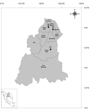
The data consists of daily rainfall data in Kelantan, Malaysia from the year 1971 to 2012. This data of 42-year period is the longest available data that have been provided by the Department of Irrigation and Drainage, Malaysia. In this study, data from three rainfall stations in Kelantan
are considered, namely Stesen Pertanian Melor (A: 5.9639◦S, 102.2917◦E), Ladang Lepan Kabu
(B: 5.4597◦S, 102.2306◦E) and Rumah Pam Salor (C: 6.0181◦S, 102.1778◦E). Figure 1 shows the location of the selected stations.
Figure 1. The geographical location of the three rainfall stations in Kelantan.
3. Methodology
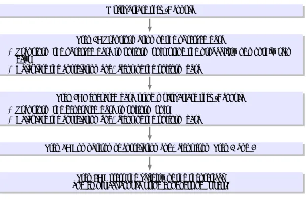
The flow of study is given in figure 2. Basically, the procedure for generating synthetic
rainfall data using multivariate skew-t copula involves four steps. The first step involves the
transformation of the observed data to uniform unit using the probability of monthly rain days. Once the data are transformed to uniform unit, the correlation coefficient is calculated. The
next step involves generating synthetic rainfall data using multivariate skew-tcopula. Similarly,
the generated data are then transformed to uniform unit and the correlation coefficient is calculated. Finally, the correlation coefficient of the observed and generated data are compared. An appropriate goodness of fit test is conducted to assess the fit between the theoretical (fitted) and empirical (observed) copula.
The monthly rainfall amount is transformed to uniform unit using the probability of monthly rain days which the data lies between 0 and 1. The term ‘rain day’ is used to denote a day on which a station has recorded 0.1 mm or more rainfall amount. The daily rainfall data series of three rainfall stations located in Kelantan region are assembled and analysed for the probability
of monthly rain days, Pk using the
Pk =
ri
R, k =1,2,· · ·,N (1)
where N is the number of rainfall station, ri is the number of rain days in a month i and R is
Multivariate skew-t copula
Step 1: Transformation of the observed data
• Transform the observed data to uniform unit using the probability of monthly rain days
• Calculate the correlation coefficient of the uniform data
Step 2: Generated data using multivariate skew-t copula
• Transform the generated data to uniform unit
• Calculate the correlation coefficient of the uniform data
Step 3: Comparison of correlation coefficient from Step 1 and 2
Step 4: Assess the validity of the theoretical and empirical copula using goodness of fit test.
Figure 2. Flow of study.
monthly rainfall amount that is generated using multivariate skew-t copula can represent the
rainfall data in actual or probability form. 3.1. Copulas
The copula approach is a useful tool to investigate the statistical behaviour of dependent
variables. If C : [0,1]d → [0,1] is a d-dimensional copula and if Fk : [0,∞) → [0,1] for
each k =1,2, ...,d is known as 1-dimensional cumulative density function (CDF) and we define
Fk :[0,∞)d → [0,1] by
F(x1,· · ·,xd) = C(F1(x1),· · ·,Fd(xd)) = C(u1,· · ·,ud)
then F is then a joint CDF for thed-dimensional random variable X= (X1,· · ·,Xd) on (0,∞)d
where ud =Fd(xd) with ud ∼U(0,1). Therefore,
P(X1 ≤ x1,· · ·,Xd ≤ xd)=C(F1(x1),· · ·,Fd(xd)) (2)
and
P[Xk ≤ xk]=Fk(xk). (3)
Note that ifUk = Fk(xk) for each k =1,2,· · ·,d and Ud is in uniform unit distributed on [0,1] therefore, the copulaCis the distribution of the vector for the random variableU=(U1,· · ·,Ud)T
[11]. In order to measure the spatial dependence between the rainfall stations, the Spearman’s correlation coefficient is used. The Spearman’s correlation coefficient of the joint distribution are defined as b ρk,l = E[(Uk−1/2)(Ul−1/2)] p E[(Uk −1/2)2(U l−1/2)2] =12E[UkUl] −3 (4)
4
for each 1≤ k <l ≤ d.
3.2. Multivariate skew-t distribution
The skewed Student’s t distribution is based on multivariate Student’st distribution that have
proven to be useful in modelling data with asymmetric and heavy tail behaviour such as rainfall
data. The multivariate skew-t distribution generalises the univariate skew-t distribution in
the same manner as the multivariate normal distribution generalises the univariate normal
distribution. The multivariate skew-t distribution with ν as the degree of freedom, µ and γ
be the parameter vectors and Σis the real positive semi-definite matrix can be represented by
the probability distribution function (PDF) as
f (x;ν, µ, γ,Σ)= Lc Hλν+2d p(ν+ρ(x)) (γ0Σ−1γ)e(x−µ)0Σ−1γ p (ν+ρ(x)) (γ0Σ−1γ)− ν+d 2 1+ ρ(2x) ν+2d (5)
where ρ(x)=(x−µ)0Σ−1(x−µ) and Lc is the normalising constant given as
Lc =
20−ν+2d Γ ν2(πν)d2 |Σ|12
. (6)
The Hλ is the modified Bessel function of third kind, denoted as Hλ(x), x >0 with indexλsuch
that Hλ(x)= 1 2 ∫ ∞ 0 yλ−1e−x2(y+y −1) dy. (7)
The mean of multivariate skew-t is given as E(x) = µ+ γνν−2 and covariance, Cov(x) =
ν
ν−2Σ+γγ
0 2ν2
(ν−2)2(ν−4). The multivariate skew-t distribution of x, where x is the d-dimensional
random vector are distributed as x ∼ Std(µ, ν,Σ, γ). Since the copula remains invariant under
any series of strictly increasing transformations of the components of x, thus it follows that the
Std(µ, ν,Σ, γ) is similar to the Student’s t distribution td(ν,0,P, γ) where P is the correlation
matrix that is corresponds to the variance-covariance matrix Σ. Thus, the trivariate skewed-t
copula of x with νas the degree of freedom and correlation matrix P can be expressed as [12]
Cν,Stp(u)=Cν,Stp(u1,u2,u3)= Stν,np
Stν−1(u1),Stν−1(u2),Stν−1(u3)
(8)
where the trivariate skew-t copula is given as
Cν,Stp(u)= ∫ Stν−1u1 −∞ ∫ Stν−1u2 −∞ ∫ Stν−1u3 −∞ Lc Hλν+2d p(ν+ρ(x)) (γ0P−1γ)e(x−µ)0P−1γ p (ν+ρ(x)) (γ0P−1γ)− ν+d 2 1+ ρ(2x) ν+2d dx. (9)
whered is the three dimensional skew-tcopula. TheStν−1 is the inverse CDF (quantile function)
of univariate skew-t distribution. In this study, we proposed the algorithm for the simulation of
trivariate random variables from a skew-t copula,Cν,Stp as follow:
(i) Transform the data to uniform,U(0,1) unit.
(ii) Simulate a random variate from trivariate skew-t of independent ofz1,z2,z3.
(iii) Set ui =Stν(xi), wherei=1,2,3.
(iv) (u1,u2,u3)T ∼Cν,Stp.
4. Results and discussion
The correlations of the uniform data are calculated for all three stations. The correlation between station AB is significantly high with 0.827 meanwhile the correlation between station AC and BC are 0.629 and 0.601, respectively. The Spearman’s rho rank correlation coefficient between the data from the three stations is also calculated. The test of significance for the correlation is
based on the hypothesis test that there is no correlation between the data (ρ=0). The results
show that the P-values are all smaller than α = 0.05 for station AB (P− value = 0.00), AC
(P−value=0.00) and BC (P−value= 0.00). Thus, we may conclude that there is statistically
significant correlation at 5% significance level among the rainfall stations. Thus, it indicates a strong spatial dependence between each station.
Next, the data are generated using multivariate skew-t copula with sample size of 104. The
effect of the parameters, that are the skewness(γ), correlation(ρ)and degrees of freedom(ν)on
the correlation (r) of the simulated data are noted. The correlation coefficient of the observed
data will be matched with the correlation coefficient of the simulated data. In each iteration, the value of the simulated correlations will be recorded.
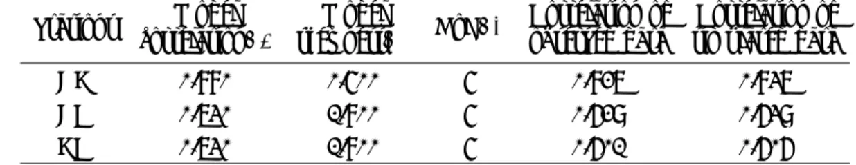
Table 1. Comparison of the correlation values of the observed (probability of monthly rain
days) and simulated data using multivariate skew-t copula.
Stations Model correlation, ρ Model skewness,γ DoF, ν Correlation of observed data Correlation of simulated data AB 0.880 0.500 5 0.827 0.837 AC 0.730 1.800 5 0.629 0.639 BC 0.730 1.800 5 0.601 0.606
Figure 3. Comparison of the fit theoretical and empirical copulas using probability of monthly rain days.
As pointed by [13], increasing the correlation of model parameters will increase the correlation of the simulated data. Meanwhile, increasing the skewness will decrease the correlation of the simulated data. However, varying the degrees of freedom just give a slight effect on the simulation results. The process is repeated until the correlation of the generated data is close enough to the correlation of the empirical data. The summarised results based on the best settings are given in table 1. The set of parameters that may best match the observed statistics are found to be ρ1 =0.88, ρ2 =0.73, ρ3 =0.73 with skewness of γ1 = 0.50, γ2 =1.80, γ3 =1.80 and ν=5 which give the simulated correlation ofr12=r21=0.837,r13=r31=0.639 and r13=r31=0.606.
6
In comparison, the correlations of the observed data arer12=r21=0.827,r13=r31=0.629 and
r13=r31=0.601, respectively.
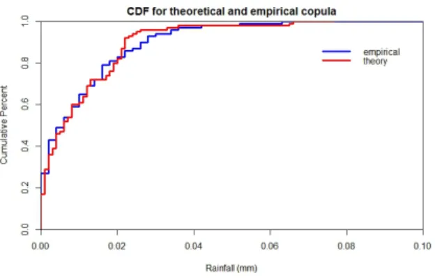
Figure 4. CDF of theoretical and empirical copulas using probability of monthly rain days. Next, we use a graphical method to evaluate the goodness of fit between the observed and the generated data. Figure 3 and 4 show the comparison of the fit between theoretical and empirical copulas and also the CDF using the probability of monthly rain days, respectively. Figure 3
shows that all the points are scattered along the straight line of y= x while figure 4 shows that
both of the empirical graph using the probability of monthly rain days and generated data using
multivariate skew-t fit closely to each other which might be a good indicator that both of the
fits are not significantly different. Thus, simulated data using multivariate skew-t copula can
be used to represent the probability of monthly rain days in a study region. Hence, this finding gives us more options on handling missing rainfall value that is related to the number of rain days at a particular location.
5. Conclusion
This study demonstrates that the multivariate skew-tcopula is suitable for modelling probability
of monthly rain days with strong correlated stations. The generation of synthetic rainfall data is important as it enables the generation of rainfall amount which has similar characteristics to the observed data. Thus, this gives us more options in handling the missing rainfall data for application in related fields.
Acknowledgement
This study was supported by Universiti Malaysia Pahang (RDU160117).
References
[1] Azzalini A and Capitanio A 2003Journal of the Royal Statistical Society: Series B (Statistical Methodology) 65367–389
[2] Zakaria R, Boland J and Moslim N 2013 Comparison of sum of two correlated gamma variables for Alouini’s model and McKay distribution 20th International Congress on Modelling and Simulation. Modelling and Simulation Society of Australia and New Zealand pp 408–414
[3] Vernieuwe H, Vandenberghe S, De Baets B and Verhoest N 2015Hydrology and Earth System Sciences 19 2685–2699
[4] Um M J, Joo K, Nam W and Heo J H 2017International Journal of Climatology 372051–2062 [5] Wong G, Lambert M, Leonard M and Metcalfe A 2009Journal of Hydrologic Engineering15129–141 [6] Ibrahim K, Zin W Z W and Jemain A A 2010ANZIAM Journal 51555–569
[7] Zakaria R, Metcalfe A, Piantadosi J, Boland J and Howlett P 2010ANZIAM Journal51231–246 [8] Madadgar S and Moradkhani H 2011Journal of Hydrologic Engineering18746–759
[10] Yee K C, Suhaila J, Yusof F and Mean F H 2014 Bivariate copula in fitting rainfall dataProceedings of the 21st National Symposium On Mathematical Sciences (SKSM21): Germination of Mathematical Sciences Education and Research towards Global Sustainability pp 986–990
[11] Nelsen R B 2013An introduction to copulas (Springer Science & Business Media)
[12] Kotz S and Nadarajah S 2004 Multivariate t-distributions and their applications (Cambridge University Press)
[13] Radi N F A, Zakaria R, Piantadosi J, Boland J, Zin W Z W and Azman M A z 2017 Water Resources Management 311729–1744