3D Facial Image Comparison using Landmarks

3D Facial Image Comparison using Landmarks

A study to the discriminating value of the characteristics

of 3D facial landmarks and their automated detection.

Alize Scheenstra

Master thesis: INF/SCR-04-54 Netherlands Forensic Institute

Institute of Information and Computing Sciences Utrecht University

3D Facial Image Comparison using Landmarks

A study to the discriminating value of the characteristics

of 3D facial landmarks and their automated detection.

Alize Scheenstra

Master thesis: INF/SCR-04-54 Netherlands Forensic Institute

Institute of Information and Computing Sciences Utrecht University

February 2005

Front Page Image

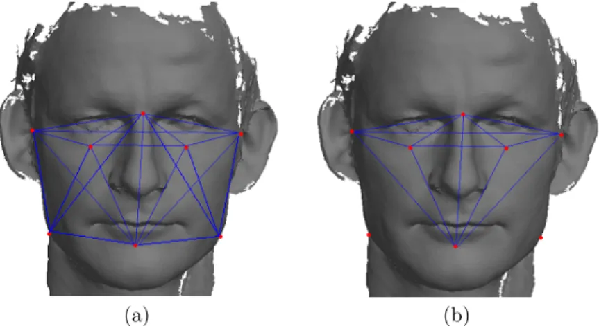
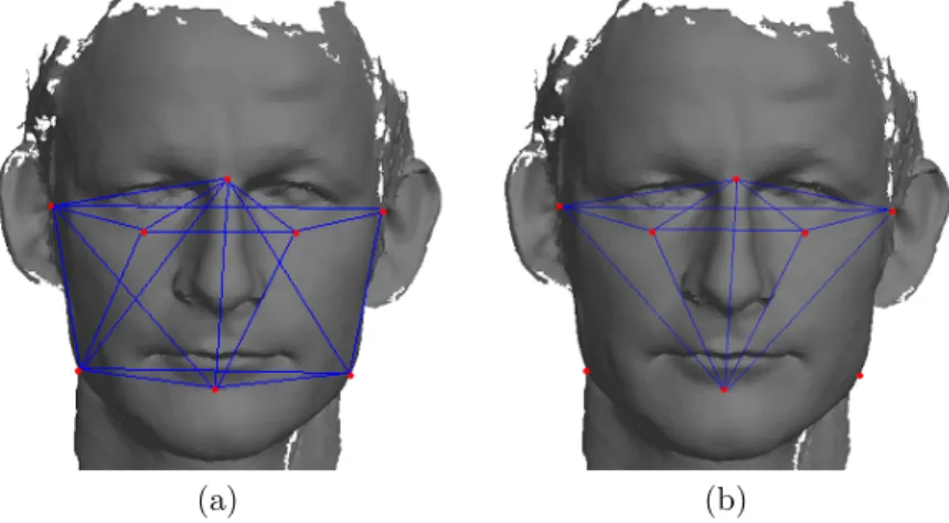
The front page image consist of three 3D facial scans. These scans are provided to me by the Netherlands Forensic Institute and are in this thesis only used for illustration purposes. The topmost face is an illustration of the landmarks that were included in the automated landmark detection. The other two faces show the distances between the landmarks that were included in the final landmark set. They are marked on two different scans to illustrate the small variations between subjects.

abstract

Many researches have been dealing with the face recognition challenge of the great variability in head rotation and tilt, lighting intensity and angle, facial expression, aging, etc. The last few years more and more 2D face recognition algorithms are improved and tested on less than perfect images. However, 3D models hold more information of the face, like surface information, that can be used for face recognition or subject discrimination. Another major advantage is that 3D face recognition can be made pose invariant. In this thesis a literature survey is presented on recent face recognition algorithms.

One way of performing 3D face recognition and face comparison, is to make use of facial landmarks. To study the possibilities of automated landmark de-tection, we first performed an analysis to find the landmarks that are best suited for automated facial comparison. We used 3D data from the facial area of 3D whole body scans, acquired in the Netherlands for the CEASAR-survey. At the time of 3D scanning, 8 facial landmarks were manually annotated, and recorded in the scanning process. We measured the absolute distances between these landmarks in the 3D model. The analysis of the measurements was performed in two ways: First, we analyzed the variance and correlation of distances be-tween facial landmarks. Second, we used the Fisher discriminant analysis to find the most significant landmark distances. The resulting sets were almost equal and can both be used for facial comparison. The most informative distances appeared to be the distances from and to the gonion (posterior point of the jawbone). Unfortunately, the gonion is found by palpation of the underlying jawbone, and therefore it cannot be found in a 3D model. The next most infor-mative are the distances from and to the sellion (point of greatest indentation of the nasal root depression) or the supramenton (point of greatest indentation of the mandibular symphysus).

To find a measure of the discriminating value of the distance measurements of the CEASAR data, we calculated the probability that the measurements of two subjects are not significantly different. We assumed that the measurements for all subjects are normally distributed. If the measurements of a subject are close to the mean (i.e. a ’common’ face), there is a probability that the same measurements are found in 1 of 2 subjects. If the measurements of a subject are in the tail of this distribution (i.e. a rare face), the probability that the same measurements are found on another subject is at most 1 in 19 subjects.

We also present an algorithm for the automated detection of 11 facial land-marks: 8 facial landmarks from the CAESAR-survey and the pronasale (nosetip) and the left and right alar curvatures (point indicating the facial insertion of the nasal wingbase). For the 8 facial landmarks is the local curvature analyzed by using bump hunting. The resulting classification rules are used for the detec-tion of these landmarks in combinadetec-tion with the geometrical informadetec-tion of the face. The pronasale and alar curvature are detected by using only the geomet-rical information of the face. We used a lower bound to indicate the detection performance of the algorithm: The pronasale and the sellion are detected best with a lower bound 66%, the gonion is detected worst with a lower bound of 0.0%. Based on the results we can conclude that this algorithm performs best on landmarks with a typical local surface (like the sellion or the left and right alar curvature) instead of landmarks with a flat local surface (like the gonion and infraorbitale).

Acknowledgements

I would like to thank a few people, who supported me during my project in many ways. First of all I thank my supervisors for their intellectual and men-tal support: Arnout Ruifrok and Jurrien Bijhold at the Netherlands Forensic Institute and Remco Veltkamp at the Utrecht University. They have provided new ideas and information, but also critical remarks when needed. Secondly, I would like to thank Ivo Alberink for his support, patience and feedback on statistical issues. Also, I would like to thank Hein Daanen and Koen Tan from TNO for providing me information and answering my questions concerning the CAESAR-survey and dataset.

Furthermore, I have to say ’thank-you’ to all my colleagues at the Nether-lands Forensic Institute for the pleasant time during working hours, but also for the interesting conversations on wednesday-evenings in the most attractive bar of Rijswijk. Finally, I would like to thank all my friends and family, partic-ularly Sander Groenendijk, for supporting me mentally and for listening to all my remarks on the progress of my graduation.

Contents

2.2 Statistical Approaches . . . 9

2.2.1 Eigenfaces . . . 9

2.2.2 Linear Discriminant Analysis . . . 9

2.2.3 Deformable Templates . . . 10

2.2.4 Other Methods . . . 10

2.3 Machine Learning Approaches . . . 12

2.3.1 Face Bunch Graph Matching . . . 12

2.3.2 Support Vector Machines . . . 12

2.3.3 Other Methods . . . 13

2.4 Other Approaches . . . 13

2.4.1 Intensity Based . . . 13

2.4.2 Infra-Red Images . . . 14

2.5 3D Models . . . 14

2.5.1 Surface Based Approaches . . . 14

2.5.2 Template Matching Approaches . . . 15

2.5.3 Other Approaches . . . 16

2.6 Discussion and Conclusion . . . 16

3 Data and Materials 19 3.1 Data Description . . . 19

3.2 Procedures of Acquiring 3D Whole Body Scans . . . 19

3.2.1 Materials . . . 20

3.2.2 Scanning Process . . . 21

3.2.3 Post processing of the Point Clouds . . . 21

3.3 Sanity Check . . . 22

3.3.1 Previous Study . . . 22

3.3.2 Errors in the Dataset . . . 23

3.4 Discussion and Conclusion . . . 26

4 Landmark Analysis 29 4.1 Information of a Landmark Set . . . 29

4.2 Information Measures . . . 30

4.2.1 Variance and Correlation based Information Measure . . . 30

4.2.2 Fisher Discriminant Analysis . . . 33

4.3 Experiments . . . 34

4.3.1 Variance and Correlation based Information Measure . . . 35

4.3.2 Fisher Discriminant Analysis . . . 38

4.5 Error Analysis . . . 40

4.6 Discussion and Conclusion . . . 42

5 Landmark Detection 44 5.1 Automated Landmark Detection . . . 44

5.1.1 Surface Characterization . . . 45

5.1.2 Landmark Detection Rules . . . 46

5.1.3 Landmark Detection Algorithm . . . 47

5.2 Performance and Results . . . 50

5.3 Discussion and Conclusion . . . 52

6 Conclusion 55 6.1 Conclusion . . . 55

6.2 Further Research . . . 56

References 58 A Landmarks of the CAESAR-survey 67 B Multiple Analysis of Variance 73 B.1 MANOVA . . . 73

B.2 nested MANOVA . . . 73

C Selection Order of the Landmark Set 75 C.1 Variance Analysis . . . 75

C.2 Correlation Analysis . . . 79

C.3 Fisher Discriminant Analysis . . . 81

D Bump Hunting 83 D.1 Creation of Detection Rules . . . 83

D.2 Using the Detection Rules . . . 84

E Detection Rules of Facial Landmarks 86 E.1 sellion (se) . . . 86

E.2 infraorbitale (io) . . . 87

E.3 supramenton (sp) . . . 89

E.4 tragion (tr) . . . 91

E.5 gonion (go) . . . 92

F Program Manual 95 F.1 View options . . . 95

F.2 Landmark Detection . . . 95

1

Introduction

1.1

Introduction

Although a lot of research is preformed in the area of face recognition, only a few systems can be used for forensic application and even less are actually used. Forensic application means the branch of science that uses scientific technology to assist the courts of law. This is due to the fact that a forensic scientist cannot afford to have a high false positive rate, which is mostly the case in face recog-nition systems. Also, many systems are based on facial images taken under con-trolled circumstances (same background, facial expression, high resolution, etc) where in forensic science the facial images are taken under uncontrolled circum-stances. The surveillance systems that capture an image of an offender provide mostly images of bad quality, to which a suspect must be compared. Nowadays, facial comparison is performed by a reconstruction at the crime scene, where the suspect is placed in the exact position as the offender on the surveillance video This is much trouble for the suspect but, in case of a non-cooperative suspect, also for the forensic scientist. One can avoid the trouble of the reconstruction if a 3D scan of the suspect can be used for the facial comparison with the of-fender. An experimental study was performed on this subject by Yoshido et al. [1]. They compared 3D facial scans to 2D surveillance images where they used 18 manually located landmarks combined with superimposition. This method reached an equal error rate (equal false positive and false negative rate) of 4.2 percent.

Besides a comparison between 3D scans and 2D images, one can also compare 3D facial scans with other 3D facial scans, for example for access authorization. A commercial system providing 3D face verification is lately brought onto the market by A4vision [2]. In this thesis we examine the possibilities of automated landmark detection for 3D facial comparison. First, we try to find a set of ab-solute distances between facial landmarks that can be used for facial comparison and we determine their discriminating value. To find a set of distances between facial landmarks, we propose two measures; one measure based on the variance and correlation of those distances and one based on the Fisher discriminant analysis. Second, we present an algorithm for the automated landmark detec-tion of 11 landmarks. The algorithm is based on prior informadetec-tion of the local surface of the landmarks combined with geometrical information. The prior in-formation is based on the manually located landmarks of the CAESAR-survey and analysed with bump hunting.

1.2

Overview of Thesis

This thesis is organized as follows: In section 2 an introduction is given on face recognition by describing the recent developments in 2D and 3D face recognition algorithms. The 3D whole body scans of the CAESAR-survey used for the experiments are described and tested for errors in section 3. In section 4 we proposed a new measure to find a set of distances between landmarks that are suited for facial comparison, based on the absolute distances between those landmarks. Also, a discriminating value is calculated for the landmarks. The proposed landmark detection algorithm is described in section 5. In section 6 conclusions and recommendations for further research will be made.

2

Related Work

One of the earliest face recognition method was presented in 1966 by Bledsoe [3]. In one of his papers [4], Bledsoe described the difficulties of the face recognition problem:

”This recognition problem is made difficult by the great variability in head rotation and tilt, lighting intensity and angle, facial expression, aging, etc. Some other attempts at facial recognition by machine have allowed for little or no variability in these quantities. Yet the method of correlation (or pattern matching) of unprocessed optical data, which is often used by some researchers, is certain to fail in cases where the variability is great. In particular, the correlation is very low between two pictures of the same person with two different head rotations.”

Since that time many researches have been dealing with this subject and have been trying to find an optimal face recognition method. In this section an overview is presented of the latest, most important face recognition methods. The main purpose of this overview is to describe the recent face recognition algorithms on still images. Previous face recognition surveys were presented by Samal and Iyengar [5], Chellappa et al. [6] and Zhao et al. [7]. In the Vendor Test 2002 the performance of different commercial face recognition methods were compared [8]. Most commercial face recognition systems use one or more algorithms as presented in the literature. However, for all systems is concealed which algorithm is used in their application. So, the commercial systems are excluded in this survey.

2.1

Metrics and Performance Measures

In this section we adapt the nomenclature of the FERET Vendor Test 2002 [9]. The face recognition problem can be separated in two different subproblems: face identification If a facial image must be identified an algorithm computes

the identification scores for all images in the dataset. These scores are ranked from best match to worst match. The k-rank recognition rate is the fraction of correct matches that are returned between rank 1 and rank

k. A rank one recognition rate (k=1) is used most in the literature. face authentication For face authentication a threshold is set where the

iden-tification scores are compared to. The result of a face authentication is a set of images which are recognised to be the same as the requested im-age. These results can be presented by an Receiver Operating Curve or ROC (the false acceptance rate plotted against the false rejection rate). A good measure to report is the Equal Error Rate (EER) which returns the rate for which the false acceptance rate and face rejection rate are equal. Sometimes is face authentication also called face verification.

The images from the dataset are called a target set. A target set can exist of one image for each subject or, which is the case for most target sets, multiple images for each subject. If the latter is the case, the set is called a gallery set. The images that are matched against the target set are called aquery set. The

query exists ofprobe images andimposterior images. The first are the images that have a match in the target set and the imposterior images are the images that don’t have a match in the target set.

2.2

Statistical Approaches

In most face recognition methods some principal component analysis (PCA) is used to reduce the number of feature dimensions. In this section we will only describe the methods that use PCA or some variant to decode the facial images. The face recognition or face verification is then performed by some classification method, also described in this section.

2.2.1 Eigenfaces

Kirby and Sirovich were the first to present face images by projecting them to a lower dimensionality using the Karhunen-Loeve Transform [10]. That this low-dimensional representation could be used for face recognition was first pre-sented by Turk and Pentland [11]. The face recognition based on PCA, the so called eigenface method, was one of the best performing methods [7]. A global approach of the eigenface method is described below. A good description of PCA is presented in a book on Pattern Classification by Duda [12].

The eigenface method can be separated in two parts. The first part is called the face coding step. In this step are the facial images projected to the face space by PCA where each image is represented by an n-dimensional vector. The second step is used for face recognition and is called the classification step. In the classification step the images are compared to each other by some dis-tance measure (for example the Euclidean disdis-tance) or by some classification method (for example the Support Vector Machines). The Support Vector Ma-chines are described in section 2.3.2. A few of this distance measures were compared by Navarette and Ruiz-del-Solar [13]. Pima and Aladjem proposed a new classifier called regularized discriminant analysis (RDA) that decreased the misclassification error of PCA [14]. However, when RDA was used for the classification based on linear discriminant analysis, as described in section 2.2.2, the misclassification error remained the same.

The PCA based face recognition is commonly used, although it is very sen-sitive for changes in illumination, facial expressions or pose of the head. Also many researchers are using PCA as a reference method when presenting the recognition rate of their newly proposed method.

2.2.2 Linear Discriminant Analysis

Another way of coding faces is based on Linear Discriminant Analysis (LDA), introduced by Fisher [15]. Belhumeur et al. was the first to apply LDA to face recognition [16]. His results showed a large improvement on the regular PCA based methods. For images with large illumination differences the presented LDA method had an error rate of 5% where the PCA method had an error rate of over 40%. In some articles this method was referred to under the name Multiple Class Analysis (MDA) or fisherfaces. A good description of LDA is presented in a book on Pattern Classification by Duda et al. [12].

Zhao et al. proposed a combination of PCA and LDA [17]. They found that this approach outperforms both single methods. Tested on a dataset of 298 images the combination reached a recognition rate of 95%.

A comparison between PCA and LDA was performed by Martinez et al. [18]. He claimed that PCA could outperform LDA in some cases. He performed several experiments varying the number of dimensionalities of the face space and the size of the training sample. He found that PCA is more robust to small trainingsamples than LDA. The reason for PCA to outperform LDA was that the underlying classes couldn’t be correctly represented when using a small training sample. Also Navarette and Ruiz-del-Solar [13] compared the LDA and PCA to each other. Their results supported the conclusions of Martinez. Some studies were performed to improve the results of LDA when only a few trainings images for each subject are available [19, 20, 21].

2.2.3 Deformable Templates

One of the first articles on template methods was published by Brunelli and Poggio [22]. They used template images of the eyes, nose and mouth for face recognition and reached a recognition rate of 100% on a dataset neutral frontal faces of 47 subjects.

Cootes and Taylor presented a point distribution model [23]. This point distribution model was later on presented by Lanites et al. as the Active Shape Model (ASM) [24]. The active Shape model was used to find points on a shape or contour by making constraints of that shape. In the same article the Active Appearance Model (AAM) was presented. The benefit of an AAM was that it took the intensity values instead of a point distribution model. On a dataset of 200 images the ASM only had a recognition rate of 70%, the AAM reached a recognition rate of 84% and a combination of both reached a recognition rate of 95.5%. But when the combined method was tested on a difficult dataset with occlusion images of 90 subjects a recognition rate of 48% was reached. The AAM and the ASM were extensively described in a recent technical report of Cootes and Taylor [25].

Jones et al. used a variation of the AAM presented as the morphable model [26]. They showed that the morphable model is more efficient than the AAM. Their conclusions were supported by Xu et al. [27]. This morphable model was recently extended to 3D by Blanz and Vetter [28], as described in section 2.5.2. Xue et al. proposed the Bayesian Shape Model that adds prior information to the Active Shape Model [29]. Their results showed that the BSM extracted the facial features more accurate than the ASM. Zhang et al. proposed to use a constrained shape model (CSM) instead of the active shape model [30]. They proposed to use Gabor Wavelets to fit the shape model more accurately. The average error rate decreased by this adjustment from 3.10% (normal ASM) to 1.94% (CSM). The same idea was also proposed by Jiao et al. under the name W-PCA and was only applied to decode the faces [31].

2.2.4 Other Methods

Many variations on PCA and LDA were proposed in literature. All methods were presented with one purpose; making the existing methods more robust to illumination and pose changes. One way of dealing with illumination was to

exclude the first largest eigenvectors from the PCA method, since they coded most of the illumination variation in a face [16]. An improvement of removing the largest eigenvectors was proposed by Kim et al. [32]. They proposed to apply independent component analysis (ICA) of the subspace remaining after the largest eigenvectors were removed. Their results showed that the error rate of their proposed method was lower than the baseline PCA method, but higher than the baseline LDA method or second-order PCA [33].

Hwang et al. compared four variations of PCA to each other: PCA, Cor-relation, PCA without first three parameters and LDA on a database of 300 subjects [34]. Their database consisted of only Asian persons. In their results they described how these algorithms performed under different facial expres-sions and different occluexpres-sions of the face. LDA performed best with an average recognition rate 90%. Hwang et al. also showed that correlation outperformed baseline PCA and PCA without the three most important eigenvectors.

Moghaddam et al. extended the properties of the linear discriminant analysis by using a probabilistic distance measure instead of the Euclidean distance [35]. Therefore he combined two low-dimensional subspaces, one for intra-personal changes and one for inter-personal changes, in a Bayesian similarity measure. An experiment from the FERET evaluation [36] showed that this method achieved a recognition rate of 95% for frontal images where the standard PCA method had a recognition rate of 83% for frontal images. Wang and Tang combined the face recognition method of PCA, LDA and Bayesian similarity measure from Moghaddam to one method [37]. The first results showed that the combined face recognition method had a better performance than the three separate methods. Yang applied kernel PCA (KPCA) and LDA (KLDA) to face recognition [38]. His new proposed method had an error rate that lies 2% lower than baseline PCA or baseline LDA. Zhou et al. proposed to combine the intra-personal space of Moghaddam [35] with the KPCA method [39]. Their results showed that the intra-personal subspace performed better than the PCA, LDA, KPCA and KLDA methods. The combined intra-personal method with KPCA had an equal recognition rate as the intra-personal subspace method. Other variations in subspace methods of eigenfaces were a PCA-mixture method introduced by Kim et al. [40], second order eigenfaces introduced by Wang and Tan [33] and a combination of both, the second order mixture-of-eigenfaces method introduced by kim et al. [41].

Zhao and Chellappa proposed in [42] a shape-from-shading (SFS) method for preprocessing. This SFS-based method used a depth map for generating synthetic frontal images. The LDA coding was applied to the synthetic images instead of the original images. The recognition rate increased with 4% when the synthetic images were used for LDA coding instead of the original images. Hu et al. proposed to use one neutral frontal image to create a 3D model to create synthetic images under different poses, illuminations and expressions [43]. Using this 3D model instead of the normal faces to apply PCA or LDA the recognition rate increased with an average of 10% for the half-profile images. A similar idea was proposed earlier by Lee and Ranganath where they presented a combination of an edge model and color region model for face recognition after the synthetic images were created by a deformable 3D model [44]. Their method was tested on a dataset with 15 subjects and reached a recognition rate of 92.3% when 10 synthetic images per subject were used and 26.2% if one image for each subject was used.

Guntruk et al. used super-resolution before projecting the faces to the eigenspace [45], he called his method eigenface-domain super resolution face recognition. Compared with pixel-domain super-resolution face recognition methods [46, 47, 48], the eigenface-domain super-resolution improved the recog-nition rate with 30%. Jin et al. proposed to combine the Foley-Sammon trans-formation and the LDA to find optimal discriminant vectors which were uncor-related to each other [49]. Tested on the databases of ORL and NUST603, their method reaches an error rate of 2.5% and 1.5% respectively.

2.3

Machine Learning Approaches

Different Machine Learning Approaches were presented during the past years. These approaches were not only used for face recognition, but also for gender classification, expression recognition, et cetera. In this section we will discuss the approaches that were presented for face recognition.

2.3.1 Face Bunch Graph Matching

Wiskott et al. introduced the Gabor Wavelets for face recognition. In their first article they presented how Face Bunch Graphs were able to describe a face [50]. A few years later a full face recognition method was presented based on these Gabor wavelets [51]. With this method Wiskott et al. reached a recognition rate of 98% on frontal images of the FERET database. For profile images a recognition rate of 84% was reached, but for half profile images the recognition rate was 57% [51]. The method was tested on a dataset of 250 subjects. 2.3.2 Support Vector Machines

As mentioned before in section 2.2, the support vector machines have been used in face recognition as a classification method after the face coding step. Mostly, principal component analysis was used for the face coding step. Support Vector Machines (SVM) were trained to distinguish between different classes or subjects by placing a hyperplane between the different classes to minimize the risk of misclassification. Detailed descriptions on SVMs were published by [52, 53, 12]. Jonsson et al. have compared the support vector machines with other com-mon classification systems used after the decoding the faces by PCA [54]. They found out that when PCA is used as a face decoder, the support vector ma-chines were outperforming nearest neighbor and correlation methods because SVM could find the discriminating vectors for discriminating between classes. However, when LDA was used for the decoding of the faces the relevant discrimi-nating vectors were already extracted by LDA and the support vector machines performed equally as the nearest neighbor or correlation. Their conclusions were supported by Saedghi et al. who performed an equal test on the European BANCA database [55].

Lee et al. proposed to improve the performance of SVM by combining the SVM classifier with the nearest neighbor rule [44]. Their approach reached the recognition performance of the SVMs but had the low computational costs of the nearest neighbor rule. Costen and Brown used an appearance model as face decoder and proposed to use a sparse SVM as classifier [56]. On a database with 22 subjects their approach had a maximal error rate of 4.5%.

Heisele et al. compared one component-based approach and two global ap-proaches of SVM [57]. The first global approach didn’t take account of intra-personal changes. In the other global approach clustering was performed to model the intra-personal changes of each subject. For the component-based ap-proach 10 parts of the face were selected for recognition. Their results showed that the component based approach performs best with a recognition rate of 90% and that the clustered global approach outperformed the non-clustered ap-proach. In one of his latest publications he described how the components for the component based approach automatically can be found [58].

2.3.3 Other Methods

Marcel proposed a multi-layer perceptron (MLP) for face verification instead of the support vector machines [59]. He extracted a feature space from each image by both principal component analysis and linear discriminant analysis. Although no recognition rate was given, Marcel stated that the MLP methods performed better that the SVM method on the same samples. Yang et al. proposed to extend the Gabor Wavelet method with AdaBoost trained for intra-and extra-personal changes [60]. This approach brought back the number of features used for recognition to obtain the same recognition rate, which speeded up the computational costs.

Wang et al. presented the recognition performance of landmark based face recognition for 2D images and for 3D models [61]. To detect the landmarks in 2D images, Gabor wavelets were used and for the landmark detection in 3D models point signatures were used as described in section 2.5.1. After landmarks were detected, PCA was used as decoder method and the classification was performed by SVMs. Their results showed that 3D landmarks alone reached a recognition rate of 85% where 2D landmarks alone reached a recognition rate of 87%. If both 2D and 3D landmarks were combined they reached a recognition rate of 89%. The authors remarked that these results could also be influenced by the number of landmarks used for face recognition, since for the point signatures 4 landmarks were used, for the gabor wavelets 6 landmarks and for the combination 12 landmarks were used.

Nefian and Heyes proposed to use Hidden Markov Models (HMM) for face recognition [62]. They reached a recognition rate of 85% on a dataset of 40 subjects. In their second attempt they proposed an embedded HMM model and reached a recognition rate of 98% on the same dataset [63].

2.4

Other Approaches

2.4.1 Intensity Based

Tak´acs and Wechsler [64] proposed a method based on the edges on a face. The edges of a face were detected by a Sobel filter. The resulted images were matched based on the Hausdorff distance. Their method was tested on 320 frontal neutral images from the FERET database and it achieved a recognition percentage of 92%. Chen et al. proposed to use a probability map to indicate the probability that a landmark is placed on a particular spot in the face [65]. This probability map is combined with a simplified 3D model which holds the geometric information of the face. They claimed that their landmark finding method is more accurate than the ASM-model, although no results are given.

2.4.2 Infra-Red Images

A first face recognition method on infra-red images is performed by Wilder et al. [66]. He concluded that visible images reached the same recognition rate as infra-red images and that a fusion between both images performs best. In an-other study, Gyaourova et al. proved that face recognition with infrared light is sensitive for glasses [67]. They propose a fusion of visible images and infrared im-ages to create an face recognition method invariant for subjects wearing glasses. Pan et al. proved that for near infra-red light (wavelength between 700 and 1000 nm) the reflectance of the human skin has large differences between sub-jects but small differences on different places on the skin of the same subject. Their face recognition was tested on hyperspectral images of 200 subjects with different poses of the head. Their best result achieves a face recognition rate 90%. Recent studies on face recognition using long wave infra-red light (LWIR) were performed by Socolinsky et al. [68, 69]. Their main conclusion was that the LWIR light methods outperform statistical approaches. However, they did also mention the problem that the acquisition of LWIR images is more expensive than visible images.

2.5

3D Models

In the last few years 3D facial models could be more easily acquired since the acquisition techniques have been improved. Therefore, some face recognition methods have been extended for 3-dimensional purposes. Using 3D models one can deal with one main problem in 2D face recognition; the pose of the head. Also the surface curvature of the head can now be used to describe a face. A recent survey of 3D face recognition was recently presented by Bowyer [70]. In this chapter we will give an overview of the recent work done on the area of 3D face recognition.

2.5.1 Surface Based Approaches

Local Methods Gordon proposed to use the Gaussian and Mean Curvature combined with depth maps to extract the regions of the eyes and the nose. He matched these regions to each other and reached an recognition rate of 97% on a dataset of 24 subjects [71]. Moreno et al. used both median and Gaussian curvature for the selection of 35 features in the face describing the nose and eye region[72]. The best recognition rate was reached on neutral faces with a recognition rate of 78%.

Xu et al. proposed to use Gaussian-Hermite moments as local descriptors combined with a global mesh [73]. Their approach reached a recognition rate of 92% when tested on a dataset of 30 subjects. When the dataset was increased to 120 subjects, the recognition rate decreased to 69%.

Chua et al. [74, 75] introduced point signatures to describe the 3D landmark. They used point signatures to describe the forehead, nose and eyes. Their method reached a recognition rate of 100% when tested on a dataset with 6 subjects. Wang et al. used the point signatures to describe local points on a face (landmarks). They tested their method on a dataset of 50 subjects and compared their results with the Gabor wavelet approach [61]. Their results showed that point signatures alone reached a recognition rate of 85% where the

Gabor wavelets reached a recognition rate of 87%. If both 2D and 3D landmarks were combined, they reached a recognition rate of 89%. The authors remarked that these results could also be influenced by the number of landmarks used for face recognition, since for the point signatures 4 landmarks were used, for the Gabor wavelets 6 landmarks and for the combination of both 12 landmarks were used.

Another approach on 3D face recognition with landmarks is proposed by ˙

Irfano˘glu et al. [76]. They automatically find landmarks based on a point could template combined with the mean and gaussian curvature. The matching is done based on the euclidean distance between the landmarks of the different faces. In a dataset of 30 subjects with 3 scans per subject, they reach a recognition rate of 96.7%.

Global Methods One global method on curvature was lately presented by Wong et al. [77]. The surface of a facial model was represented by an Ex-tended Gaussian Image (EGI) to reduce the 3D face recognition problem to a 2D histogram comparison. The proposed measure was the multiple conditional probability mass function classifier (MCPMFC). Tested on a dataset of 5 sub-jects with 50 scans per subject, the MCPMFC has a recognition rate of 80% where a minimum distance classifier (MDC) reached a recognition rate of 68%. However a test on synthetic data showed that for both methods the recognition rate decreased with 10% when the dataset was increased from 6 subjects to 21 subjects.

Papatheodorou and Rueckert proposed to use a combination of a 3D model and the texture of a face [78]. They also proposed some similarity measures for rigid alignment of two faces for 3D models and for 3D models combined with the texture. Their results showed an increase for frontal images when adding a texture to the model.

Beumier and Acheroy proposed to use vertical profiles of 3D models for face recognition. Their first attempt was based on three profiles of one face and had an error rate of 9.0% when it was tested on a dataset of 30 subjects [79]. In their second attempt they added grey value information to the matching process [80]. This attempt reduced the error rate to 2.5% when it was tested on the same database. Wu et al. proposed to perform 3D face recognition by extracting multiple horizontal profiles from the 3D model [81]. By matching these profiles to each other they reached an error rate between 1% and 5.5% tested on database with 30 subjects.

2.5.2 Template Matching Approaches

Blanz, Vetter and Romdhani proposed to use a 3D morphable model for face recognition on 2D images [82, 28, 83]. With this method tested on a dataset of 68 subjects they reached a recognition rate of 99.8% for neutral frontal images and a recognition rate of 89% for profile images. Huang et al. added a component based approach to the morphable model [84] based on the approach of Heisele [58]. However, the recognition rate was for all approaches of the morphable model between the 75% and the 99%.

Naftel et al. presented a method for automaticly detecting landmarks in 3D models by using a stereo camera [85]. The landmarks were found on the 2D images by an ASM model. These landmark points were transformed to the 3D

model by the stereo camera algorithm. This algorithm was correct in 80% of all cases when tested on a dataset of 25 subjects.

A similar idea was proposed by Ansari and Abdel-Mottaleb [86]. They used the CANDIDE-3 model [87] for face recognition. Based on a stereo images landmark points around the eyes, nose and mouth were extracted from the 2D images and converted to 3D landmark points. A 3D model was created by transforming the CANDIDE-3 generic face to match the landmark points. The eyes, nose and mouth of the 3D model were separately matched during the face recognition. Their method achieved a recognition rate of 96.2% using a database of 26 subjects. Lu et al. had used the generic head from Terzopoulos and Waters [88] which they adapted for each subject based on manually placed feature points in the facial image [89]. Afterwards the models were matched based on PCA. This method was tested on frontal images and returns in 97% of all cases the correct face within the best 5 matches.

2.5.3 Other Approaches

The original principal component method for 3D facial models was implemented by Mavridis et al. for the European project HiScore [90]. Chang et al. had compared the performance of 3D eigenfaces and 2D eigenfaces of neutral frontal faces on a dataset of 166 subjects [91]. They found no real difference in per-formance for the 2D eigenfaces and 3D eigenfaces. However, a combination of both dimensionalities scored best of all with a recognition rate of 82.8%. Xu et al. proposed to use 3D eigenfaces with nearest neighbor and k-nearest neighbor as classifiers [92]. Their approach reached a recognition rate around the 70% when tested on a dataset of 120 subjects.

Bronstein et al. had proposed to transform the 3D models to a canonical form before applying the eigenface method to it [93]. They claimed that their method could discriminate between identical twins and was insensitive for facial expressions, although no recognition rates were given.

Tsalakanidou et al. proposed to combine depth maps with intensity images. In their first attempt they used eigenfaces for the face recognition and his results showed a recognition rate of 99% for a combination of both on a database of 40 subjects [94]. In a second attempt embedded hidden markov models were used instead of eigenfaces to combine the depth images and intensity images [95]. This approach had an error rate between the 7 % and 9%.

2.6

Discussion and Conclusion

It is hard to compare the results of different methods with each other since the experiments presented in literature are mostly based on different seized dataset. For example one method was tested on neutral frontal images and had a high recognition rate, while another method was tested on noisy images with different facial expressions or head poses and had a low error rate. Besides the performance of the algorithm the computational time is also important. Unfortunately, the computational costs are only mentioned in a few articles, so no correct comparison on the computational costs can be made.

Some authors presented combinations of different approaches for a face recog-nition method and these performed all a little better than the separate meth-ods. If the error rate decreases significantly, while the recognition rate increases

only a little bit, the combined method is still preferred. But if combining two methods make the computational costs increase much, this method wouldn’t be preferable at all.

Most interesting for this survey were the studies that presented a compari-son study, like [13, 54, 55]. Phillips et al. present comparicompari-son studies performed on the FERET database [8]. The latest FERET test is performed in 2002 on commercial systems [9]. The FERET test performed on different algorithms is presented in 2002 [36]. In the latter survey the computational costs were taken a little into account. An important conclusion from this survey was that the recognition rates of all methods were improved over the years. The dynamic graph matching approach of Wistkott et al. [51] had the best overall perfor-mance on identification. For face verification the combination of PCA and LDA presented by Zhao et al. [17] performed best. Although published in 2000, the test itself was performed in 1997 which makes a new recent test preferable.

An implementation of face recognition methods is published by Beveridge and Draper [96]. In their application, four different algorithms are implemented and downloadable: normal PCA, a combination between PCA and LDA [17], the Bayesian approach of Moghaddam [35] and an implementation of the Elastic Bunch Graph Matching [51]. So if one likes, one can compare these algorithms on their own dataset.

In table 1 a summary is given for the most important and successful face recognition methods. One can see that the 3D face recognition approaches are still tested on very small datasets. However, the datasets are increasing during the years since better acquisition materials become available. By increasing a dataset, however, the recognition rate will decrease. So the algorithms must be adjusted and improved before they will be able to handle large datasets with the same recognition performance. Another disadvantage of most presented 3D face recognition methods is that most algorithms still treat the human face as a rigid object. This means that the methods aren’t capable of handling facial expres-sions. In contrast of 3D face recognition algorithms, most 2D face recognition algorithms are already tested on large datasets and are able to handle the size of the data tolerable well. The last few years more and more 2D face recognition algorithms are improved and tested on less perfect images, like noisy images, half profile images, occlusion images, images with different facial expressions, et cetera. Although not one algorithm can be assumed to handle the difficult images good enough, an increasing line in performance can be found.

Although the 2D face recognition seem to outperform the 3D face recognition methods now, in future it can be the other way around. The 3D models hold more information of the face, like surface information, that can be used for face recognition or subject discrimination. Compared to 2D face recognition only a little research is performed on 3D face recognition. Therefore, 3D face recognition is still a very challenging but very promising research area.

me th o d mo dali ty reference n u m b e r of su b jec ts image s p er su b jec t rank on e recogniti on error rate v ari ation in d atase t p er su b jec t p e rf ormance in % in % in images ba selin e PCA 2D [36] 1196 1 79 ? no baselin e LD A 2D [54] 200 at le ast 4 97. 5 1.48 y es baselin e Correlatio n 2D [36] 1196 1 82 ? no PCA-LD A 2D [7] 298 1 95 ? y es Ba y esian PCA 2D [35] 1196 1 95 ? no ASM -AAM 2D [24] 30 10 92 ? no ASM -AAM 2D [24] 30 3 48 ? y es F ac e Bu nc h Grap h 2D [51] 300 1 97 ? no F ac e Bu nc h Grap h 2D [51] 250 1 84 ? y es Inf ra-Re d im ages 2D [97] 200 7 89 ? no Gau ssian im ages 3D [71] 8 3 1 00 ? no P oin t S ign atur e s 3D [75] 6 1 1 00 ? no Ex te n ded Gau ssian Images 3D [77] 5 1 8 0 ? no Pr ofil e s 3D [80] 26 1 ? 2.5 no Mor ph able m o del 3D [82] 68 21 99. 8 ? no Mor ph able m o del 3D [82] 68 21 89 ? y es 3D e ige n face s 3D [91] 166 2 83. 7 ? no 3D e ige n face s 3D [92] 120 1 71. 1 5 y es Canon ical forms 3D [93] 157 1 ? ? y es T ab le 1: A summary on most imp ortan t pr e se n te d 2D and 3D fac e recogniti on metho ds. T h e v ariati on in im ages c ol umn sho ws if image s in d e d atas et w ere tak e n u nd e r d iffe re n t cond ition s, li k e facial expr e ss ion, il lumin ation, h e ad p ose et cete ra.

3

Data and Materials

3.1

Data Description

For this thesis we used the whole body scans of the Dutch and Italian part of the CAESAR-survey [98]. The main goal of the CAESAR-survey was to acquire 3D whole body scans of 5.000 subjects. It took place from December 1997 until December 2001 in America, Italy and the Netherlands.

Each subject was scanned in three different poses; standing, relaxed seating and seating in such a way the whole body was visible for the camera. Also, demographic information was collected of each subject, like age, data collection location, date, education level, ethnic group, family income in the past year, gender, present occupation, marital status, etc. Also, 73 landmarks were man-ually placed on each subject before scanning. Besides the 3D whole body scan a separate file was available with the 3D-coordinates of these landmarks. The landmarks which were used in the CAESAR-survey, are in detail described in Appendix A

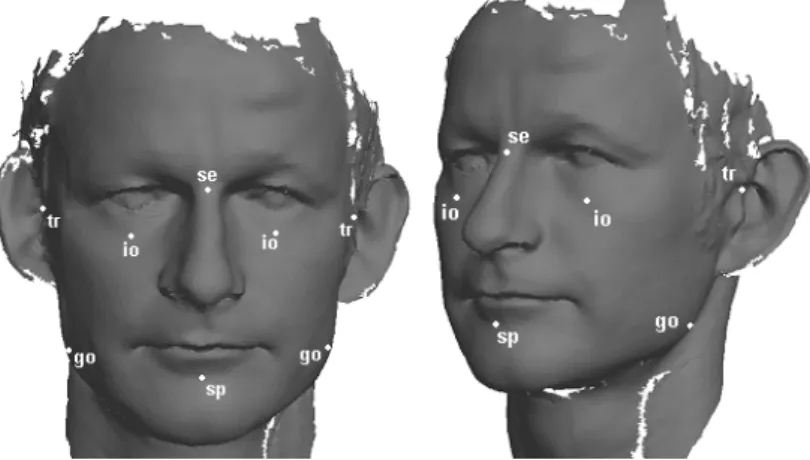
For the data analysis and the 3D face comparison problem we extracted the facial region from each whole body scan using bounding boxes as described in [99]. In this facial region 8 landmarks were defined by the CAESAR-survey:

sellion(se)Point of greatest indentation of the nasal root depression

right infraorbitale(r. io)Lowest point on the inferior margin of the right orbit, marked directly inferior to the pupil

left infraorbitale (l. io) Lowest point on the inferior margin of the left orbit, marked directly inferior to the pupil

supramenton (sp)Point of greatest indentation of the mandibular symphysus, marked in the midsagittal plane.

right tragion (r. tr) Notch just above the right tragus (the small cartilaginous flap in front of the ear hole)

left tragion (l. tr)Notch just above the left tragus (the small car-tilaginous flap in front of the ear hole)

right gonion (r. go)Inferior posterior right tip of the gonial angle (the posterior point of the angle of the mandible, or jawbone.

This point is difficult to find when covered with a lot of tissue. left gonion(l. go)Inferior posterior left tip of the gonial angle (the

posterior point of the angle of the mandible, or jawbone. This point is difficult to find when covered with a lot of tissue.

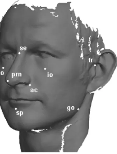
The locations of these landmarks are shown in figure 1.

3.2

Procedures of Acquiring 3D Whole Body Scans

In this section the acquisition of the 3D whole body scans and the correspond-ing landmark coordinates for the CAESAR-survey are described. Since the data collection was done in America, the Netherlands and Italy, differences in scan-ning proceduder occurred during the survey [100]. Some of these differences had an impact on the quality of the 3D whole body scans. These differences and their impact are also described here.

Figure 1: The positions of the facial landmarks of the CAESAR-survey. These landmarks are manually located (This scan is provided by the Netherlands Forensic Institute and not a part of the CAESAR-survey.).

3.2.1 Materials

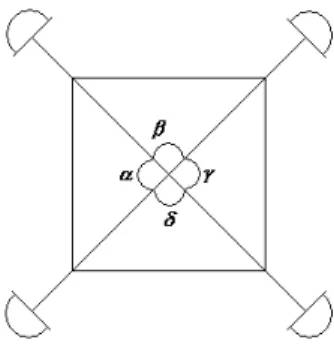
Scanning Devices Two different scanning devices were used to scan the bod-ies. In Italy and America the 3D whole body scans were acquired using a Cyber-ware 3D body scanner [101]. In the Netherlands a Vitronic 3D body scanner was used [102]. Both scanning devices have a square platform with a camera block on each corner. A camera block exist of four depth cameras and one texture camera. So, the scanning process for 1 subject resulted in 16 point clouds and 4 texture files that must be merged to one 3D whole body scan, as described in 3.2.2. In figure 2 the four camera blocks around the platform are shown. Also, the angles between the camera blocks are presented. For the Vitronic scanning device it is known that α= γ and β = δ, but that α =γ > β =δ. For the Cyberware scanner these ratios weren’t known.

The Cyberware scanning device was extensively tested and calibrated before the survey started. However, the Vitronic scanning device wasn’t tested so well as the Cyberware scanner. As a consequence, it wasn’t quite clear what the differences were between both scanning devices when the survey started [100]. These differences were revealed and dealt with during the survey.

The Vitronic scanning device had a higher scanning resolutions than the Cyberware scanning device, but the scanning volume of the Vitronic was smaller. Because of the small scanning volume of the Vitronic scanner, some body parts weren’t visible for the cameras. To solve this problem the orientation of some scanning poses were changed for this scanning device as described in section 3.2.2.

Another problem was found in the software used for the landmark picking. This software was developed for the Cyberware scanner and later on adjusted for the Vitronic scanner. The software could be applied on scans acquired by the Vitronic scanner, but only the scans that were aligned by hardware calibration. The landmark picking software couldn’t handle the software alignment of the scans, since the there was too much loss of resolution. For the Cyberware scanner the software alignment could be performed without the loss of resolution

in the landmark picking software. This means that the landmarks were more accurately picked for the scans acquired by the Cyberware scanner than for the scans acquired by the Vitronic scanner.

Landmarks To indicate the landmarks on the body white stickers and bumpers were used. The stickers were flat, round and had a diameter of 1 cm. The bumpers were little cubes with a width, height and depth of 0.5 cm and were only used at places difficult to see in the texture file, for example the landmarks on the shoulder. In this thesis to both stickers and bumpers are referred to as markers. In the Netherlands 6 observers were hired to place the markers. These observers were given all the information needed for placing the markers at the right spot on the body.

The landmark picking was done semi-automatically. A program identified the locations of the landmark based on the white color of the landmark. These locations were presented to the observer to pick the accurate location of the landmark file. It could occur that a landmark was visible on two texture files. In that case the program selected one texture file to detect the landmark location. This landmark location was presented to the observer. After the observer had picked the landmarks from the texture file, the location and landmark name were automatically written in a landmark file. To limit the amount of work the observers picked the landmarks for pose a and pose b only.

3.2.2 Scanning Process

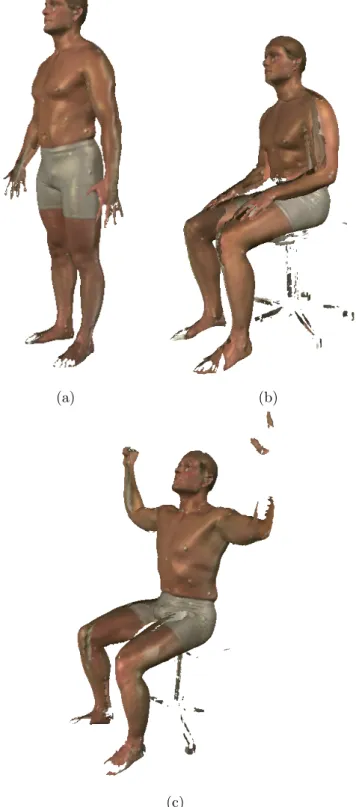
Each subject to be scanned was dressed in tight shorts. The women wore a tight top, too. By using this outfit most of the body is shown and visible for the scanner. One of the observers placed all the 73 landmarks on the body before the actual scanning. For the scanning itself each subject had to stand in three different poses. First, one was asked to stand still with the arms stretched besides the body (pose a). For the second pose (pose b) each subject was asked to sit down with his arms on his knees. For the last pose (pose c) each subject, still seating, was asked to lift his arms above his head. The three poses of the CAESAR-survey are shown in figure 4.

The resolution problems as described in section 3.2.1 lead to a change in the orientation of the scanning poses of the Dutch part of the Survey. As described before, the scanning volume of the Vitronic was small and to make most of the body parts visible for the depth cameras, pose b had to be rotated with 90 degrees. Pose a and c of the Dutch survey kept the same orientation. In fact, pose a and c had the same orientation as all three poses of the American and Italian survey. The orientations of the three poses of the Dutch survey are given in figure 3.

3.2.3 Post processing of the Point Clouds

After the scanning and landmark picking, the 16 point clouds of the depth cameras and the 4 2D-textures of the color cameras had to be aligned and merged to one object in one coordinate system with a resolution of 2 mm. For more detailed information of the aligning and merging process the reader is referred to the master thesis of Suikerbuik [103]. The landmark coordinates were also transformed from 2D coordinates on the texture to 3D-coordinates in

Figure 2: The angles between the four camera blocks of the 3D scanning devices measured from the middle of the platform.

(a) (b) (c)

Figure 3: The orientations of the three scanning positions of the Vitronic scanner were (a) shows pose a, (b) shows pose b and (c) shows pose c. The poses a and c are both directed to the angleβas shown in figure 2 and pose b is oriented in the direction of the angleγ

the same coordinate system as the whole body scan. After the transformation each landmark was snapped to the closest point in the point cloud of the whole body scan.

3.3

Sanity Check

In earlier research was found that in some cases the location of the landmarks wasn’t accurate [103, 104]. Since this dataset will be used as the ground truth during this study, one needs to know the frequency and the causes of these incorrect landmark locations.

3.3.1 Previous Study

Verbaan did a study on measurement errors introduced by the observers [105]. He found an average variation of 5 mm for placing the markers on the body for all observers. In his work Verbaan also described other errors that could oc-cur during the scanning process. He mentioned as possible errors the incorrect placement of the markers on the body, the variation in the posture of the sub-jects and the movement of the subject during scanning (as one can see in figure 4(c), where the subject had moved his left arm). Verbaan further concluded that the landmark picking in one texture could only cause a minimal error, due to an excellent zoom function.

Suikerbuik rejected this theory of Verbaan on the latter issue and concluded that observers couldn’t pick the exact centre of the landmarks with a diameter of 10 mm from a texture file correctly [103]. Even if the observer had picked a landmark correctly, the landmark locating software snapped the landmark coordinate to the closest point of the body scan, introducing a maximal error of √12_{+ 1}2_{+ 1}2 _{= 1.73 mm for each landmark. Also, Suikerbuik added the}

height of the bumpers to the possible causes of errors. 3.3.2 Errors in the Dataset

In this section is described how we tried to find other errors than described in the previous section. We tried to identify the causes of the newly found errors in the dataset. Since we were only using the facial area of a whole body scan, we restricted ourselves to validate the facial landmarks.

For our studies we were using a dataset of 20 subjects. One observer placed the landmarks on each subject before the scanning process. Next, each subject was scanned in the three poses of the CAESAR-survey (pose a,pose b andpose c) as shown in figure 4. For each pose the subjects were scanned three times under the same circumstances (same landmarks, same pose,etc). We referred to these three scans asscan 1,scan 2 andscan 3. The scanning of all subjects was done on the same day by the Vitronic scanner used in the Netherlands and by the Cyberware scanner used in America and Italy. Summarizing, the dataset existed of 20 subject with 18 whole body scans for each subject; 9 scans from the Cyberware scanner and 9 scans from the Vitronic scanner.

Empirical Approach As described in section 3.3.1, Verbaan had mostly fo-cused his research on the variation of landmarks caused by the observers. In this section we were studying the influence of scanning procedure, like described in section 3.2.2. Since we were especially interested in the distances between landmarks, we had set up an experiment to compare the distances between the landmarks for the different poses of the subjects. We had split up the dataset for the scans made by the Cyberware and Vitronic scanning devices.

Table 2 shows the results of this experiment. For each pose we had calculated the differences between the distances between the landmarks. For example, the table entry (a-b,se - sp) for the column Vitronic denotes that the average distance ’sellion - supramenton’ for all 20 subjects scanned by the Vitronic is 0.06 mm larger in pose a than in pose b.

One would expect that the average difference between two poses for a certain distance is 0.00 mm, since the subjects were scanned with the same landmarks on the body in each pose. For some table entries, however, the average lies over 4.0 mm (see table entry (a-c,sp - r go). This results suggest that there could be a systematically error in the dataset. Suikerbuik noted in his report that the landmarks were snapped to points of the point cloud, introducing an error of at most 1.73 mm [103]. We took this error into account and stated that the average difference above 2.0 mm couldn’t be explained by previous study. These distances could be influences by systematical errors (bold figures in the table).

One can see in table 2 that the distances which have more than one average difference above the 2.0 mm are in six cases distances on the left side of the face, in four cases distances on the right side of the face and in three cases distances at the frontal part of the face. It is interesting that most affected distances are

Table 2: Absolute differences in mm between two poses for the separate vari-ables. The poses are split up for scanning device.

Vitronic Cyberware variable a - b a - c b - c a - b a - c b - c se - sp 0.06 0.00 -1.01 0.06 -0.57 -0.62 Se - l tr 0.10 0.46 -0.07 0.10 -1.74 -1.84 Se - r tr 0.58 -0.76 -1.34 0.38 1.20 0.82 Se - l io 0.56 -0.17 -0.73 0.04 -0.62 -0.65 Se - r io 1.13 -0.92 -2.05 -0.64 -0.28 0.35 Se - l go -0.69 -2.80 -2.11 -0.10 -3.21 -3.11 Se - r go 2.15 -1.83 -3.98 -0.10 -0.52 -0.42 r io - l io 3.60 0.55 -3.05 0.11 -1.06 -1.17 r io r tr 1.35 1.02 -0.33 0.20 1.51 1.31 r io - sp 1.14 1.13 -0.01 1.12 -1.32 -2.44 r io - r go 2.80 -1.07 -3.87 0.33 -1.84 -2.17 l io - l tr 0.23 3.61 3.38 0.17 -0.96 -1.13 l io - l go 0.60 -1.41 -2.01 0.57 -3.78 -4.35 l io - sp 4.12 0.97 -3.15 0.26 0.05 -0.21 sp - l tr 2.32 4.04 1.72 0.25 0.40 0.16 sp - r tr -1.22 -1.30 -0.08 1.32 0.37 -0.95 sp - l go 1.63 -1.12 -2.75 0.33 -3.36 -3.68 sp - r go -1.46 -6.53 -5.07 1.05 -4.07 -5.12 r tr - r go 1.51 2.59 1.09 0.21 2.64 2.43 l tr - r tr 2.53 -0.90 -3.43 0.56 -0.64 -1.20 l tr - l go -0.43 1.60 2.03 0.19 1.72 1.53 r go - l go 2.34 3.14 0.80 -0.97 4.16 5.13

from and to the left and right gonion and found in the whole body scans of the Vitronic Scanning device.

Statistical Approach We showed in the previous section that there could be some systematical errors in the dataset. We would like have tested all factors for systematical errors, but in the dataset we used only one observer placed and picked the landmarks. So, we couldn’t test the landmark placing and landmark picking for systematical errors. However, Verbaan had performed an analysis on the variance by observers and couldn’t find any systematical errors introduced by the observers. Therefore we assume that if there is a systematical error in the dataset, it must have been introduced by the other scanning factors. Those other factors, the scanning pose and scanning device, are tested here.

In the perfect case, the factors have no significant influence to any distance and the measured distances are the same for each scanning device or scanning pose. As statistical test, we used themultivariate analysis of variance test, the so called MANOVA test [106]. The MAVONA test is explained in more detail in Appendix B. In this case we used a two level nested MANOVA with the scanning devices {Vitronic, Cyberware} and poses {a,b,c} as the factors. For each scan we measured the same distances in the face as used for the empircal approach. One can find these distances in table 2. These distances were the

variables of the MANOVA test.

We performed the nested MANOVA test separately on the 20 subjects. For each subject we tested on the first level the null-hypothesis (H0) that there is

no significant influence between the means of the cyberware and the vitronic scanner. In the next level (H1) we tested if there is a significant influence of the

scanning poses for the different scanning devices. Both hypotheses are summa-rized below:

H0: µCyberware =µvitronic:

There is no significant influence of the scanning device on the measurements.

Ha: µCyberware6=µvitronic:

There is a significant influence of the scanning device on the measurements.

H1: µa,Cyberware=µb,Cyberware =µc,Cyberware and

µa,vitronic=µb,vitronic=µc,vitronic:

There is no significant influence of the scanning poses on the measurements for each scanning device.

Ha: There is a significant influence of the scanning poses on the measurements for each scanning device.

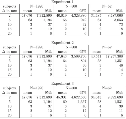
Using the Wilks’ lambda as MANOVA statistic and a significance level of 0.05, we looked at the number of subjects for which a significant influence was found. Under theH0andH1, the number of significant influences is binomially

distrib-uted with the parameters 20 (number of subjects) and 0.05 (significance level). We can calculate the critical value using thet-distribution (t(20),0.05 ≈1.725).

Now, we can say with 95% probability that in case of no significant influence, there are less or equal than 1 + 1.725∗0.975 = 3 rejections of our hypothesizes.

H0 H1

all distances 1 6

Table 3: The number of subjects for with theH0and/or theH1 were rejected

The results are shown in table 3. One can see that there isn’t a significant influence for the scanning devices, since the null-hypothesis is only rejected for one subject. On the other hand, there is a significant influence found for the scanning poses, since theH1 is rejected for more than 3 subjects.

For a second test, we partitioned all distances in three groups. The first group consisted of distances on the left part of the face, the second group con-sisted of distances at the right part of the face and the last group concon-sisted of distances at the front part of the face (se - sp, l io - r io, l tr - r tr and l go - r go). We performed this test based on our observations in the empirical approach that there appeared to be a difference in distances at the left, right and frontal parts of the face. This effect can be found in table 2. For each group we performed the same tests as described above. The results of these tests can be found in table 4.

One can see in table 4 that there is a significant influence for the scanning devices and the scanning poses for the left, right and the frontal distances. In contrast with the observation in the empirical approach where it seems that

H0 H1

left 19 14 right 13 11 frontal 8 9

Table 4: The number of subjects for with theH0and/or theH1 were rejected

only the right distances were affected with errors, there is a significant influence found for the left as well as the right distances.

Another remarkable fact is that the scanning device has a significant effect for the three separate groups (left,right and frontal distances). This is in contrast with our first test, where all distances are placed in one group and no significant influence for the scanning device is found. If one compares the number of rejections from the first experiment with the second experiment, one can see that the number of rejections for the second experiment is much larger.

3.4

Discussion and Conclusion

In this section we have discussed the dataset that will be used for analysis and later on for the automated landmark detection. We have described the scanning procedure and we discussed the differences between the Cyberware scanning device and the Vitronic scanning device and the differences of scanning procedures caused by the differences in scanning.

We performed an empirical test as well as a statistical test to prove that the measurements on the landmarks are significant influenced by the scanning devices and the scanning poses. The empirical test showed us there could be a systematical error of 5 mm for some distances occurring under different scanning poses and device. It also showed that a little more distances on the left part of the face could be affected with this error. With the statistical MANOVA test we showed that the scanning pose had a significant influence on the measurements for some distances. However, for the scanning device was no significant influence found.

Since the empirical test showed a difference between the left and right part of the face, we had split up the distances and performed the MANOVA test again on the separate groups. It was now shown that the distances at the left part of the face as well as the right part were both significantly influenced by the scanning pose and also the scanning device. For both left and right distances significant influences were found, we noticed that the number of rejections for the separate distances was much larger compared to the number of rejections for all distances together. It could be possible that the distances at one part of the face neutralize the systematical errors at the other part of the face. More research on this area is needed on this topic.

So, we have shown that the dataset of the CAESAR-survey contains sys-tematical errors for some distances in the face. These syssys-tematical errors result in a displacement of a landmark of at most 5 mm. In our following research we handle these systematical errors as if they are a part of the intra-variance of a measurement. More details on this topic is described in the next section. In that section we use the dataset from the CAESAR-survey for our landmark analysis.

We have proved in this section that there were significant influences caused by some scanning factors. But, we have not yet discussed what the causes of these differences were. In this research we found two problems that could be the cause of the systematical errors.

First, the errors could be caused by the scanning position. As one can see in image 3(b) and can read in section 3.2.2, the head of the subject isn’t placed in the middle of the scanning area due to the non-optimal scanning volume of the Vitronic scanner. Since the texture cameras couldn’t get a clear view of the side (depth) of the face, no optimal texture file could be produced for the head of each subject. So the observers that picked the landmarks from the texture files weren’t capable of accurately picking the landmarks that were placed in the depth of the face, like the tragion and the gonion. This could introduce an error and it could explain why the left and right gonion appeared to be most influenced by the scanning factors. This could also be the case for the Cyberware scanner, since it wasn’t exactly known how the subjects were placed on the scanning platform. We only know the orientation of the subjects for each pose.

Second, we know that the landmark picking software could only be used for the Vitronic scanner before the software alignment was done. This is described in more detail in section 3.2.1. So, only a hardware calibration was performed on the 3D model before the landmark picking. After the landmark picking, the software alignment for the 3D model is performed as described in [103]. When the software alignment is finished the texture file is wrapped over the 3D model and the landmarks are snapped to some model points. But, the transformation of the model caused by the software alignment wasnt performed on the landmark points, so these landmark points could be snapped at the wrong spot in the model.

Especially, the second error cause could explain why the Vitronic scanning device shows more errors than the Cyberware scanning device in our empirical approach. The first error cause could have occurred for both scanning devices and could explain why both scanning devices show systematical errors. More research on this topic should point out what the exact cause of the systematical errors was.

(a) (b)

(c)

Figure 4: The three scanning poses. position a: pose (a), pose b: relaxed seating (b) and pose c: best scan coverage seating (c)

4

Landmark Analysis

4.1

Information of a Landmark Set

When using landmarks for face recognition, a lot of information of the face isn’t used. So, the locations of the landmarks should be chosen carefully to use as much facial information as possible. Besides the location of the landmarks the number of landmarks must be carefully picked as well. More landmarks will give more information about a face so the face comparison method will perform better. But when using too many landmarks, there is a risk of creating a landmark set that uses noise in the classification process. In this case, there will be a high false reject rate.

This chapter describes different approaches for selecting a set of distances between landmarks that will give us as much information as possible, but uses no information that can be considered as noise. To measure the amount of information of a set we propose to make use of formulas for each analysis method. Each setS consist of distances between landmark points, from here on referred to as landmark set. The number of elements in the set is described byN. Each landmark set gives a certain amount of information of a face. The information of a landmark set is therefore described by I(S). In this section two different measures are used to find a landmark set. The first method is a measure based on the variance and correlation and is described in section 4.2.1. The second method is an existing method based on the Fisher discriminant analysis and is described in section 4.2.2

The user must decide which set is selected as the final landmark set. This can be done by using a threshold T. This threshold can be a maximal accept-able number of elementsTN in the final landmark set or a minimal acceptable increase in informationTI(S). In this thesis the final landmark set is found using

a bottom-up approach. We start with an empty set and elements are added to the set which will give the highestI(S), this will continue until the manual set threshold T is reached. The algorithm used is described in the pseudo code below.

Algorithm for selecting a set of landmarks

LIST candidateLandmarks <- all distances between all landmarks LIST landmarkSet <- empty

while( I(landmarkSet) < T || Length(LandmarkSet) < T ) do {

bestElement <- candidateLandmarks.first(); bestInformation <- I(landmarkSet + bestElement);

for (element e in candidateLandmarks) do {

if( I(landmarkSet + e) > bestInformation ) {

bestInformation <- I(landmarkSet + e) bestElement <- e;

} }

candidateLandmarks = candidateLandmarks - bestElement; landmarkSet = landmarkSet + bestElement;

if(candidateLandmarks.empty() = TRUE) break();

}

return landmarkSet;

4.2

Information Measures

Many different methods can be used as information measures. For our analysis, we have chosen for two information measures. First, we propose an information measure based on variance and correlation between the landmarks and second, we will use the Fisher discriminant analysis as reference method for our proposed approach. Both information measures are described shortly in this section. 4.2.1 Variance and Correlation based Information Measure

In our proposed information measure, the distances are selected based on their variance and correlation. First, the variance analysis is used to add the distances between landmarks to the set. After our variance analysis we will test the resulting set on correlation between the elements. If two elements are highly correlated, the distances will add very little information to the set. So, these elements should be excluded from the set. We chose to test first on variance since the correlation approach will first add noise to the set, since noise is uncorrelated. Now, the variance analysis is used to filter the noise from the landmark set.

Variance Analysis When one attempts to measure a ground truth, there is always some variance in the measurements. One can divide this variance into

inter-variance andintra-variance. The inter-variance of distances between land-marks is the variation in measurements on different subjects. The discriminating value of landmark distances grows when the inter-variance grows. The intra-variance is the variation in different measurements on the same subject. It is sometimes called the measurement error or the uncertainty margin of a measure-ment. If the intra-variance of a distance is relative large to the inter-variance, the discriminating value of that landmark distance will be low. The low discrim-inating value is due to the large amount of overlap of the intra-variance with the inter-variance, so it is difficult to tell whether two measurements belong to the same subject or two different subjects.

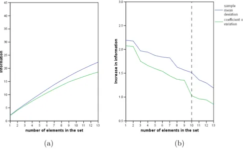
For the selection of distances between landmarks we are looking for distances having a small intra-variance and a large inter-variance. In other words we are looking for landmarks on places where human faces differ a lot and which are easy to find in a face. To deal with these kind of information, we define information of a landmark setI(S) of withN elements as the ratio of the inter-and intra-variance as described in (1).

I(S) =