Data Visualization within Urban Models

Data Visualization within Urban Models

Anthony Steed

, Salvatore Spinello

, Ben Croxford

, Richard Milton

1

_{Department of Computer Science, University College London, UK}

_{LaBRI, Université Bordeaux, France}

3

_{Bartlett School of Architecture, University College London, UK}

A.Steed@cs.ucl.ac.uk, spinello@labri.fr, B.Croxford@ucl.ac.uk, R.Milton@cs.ucl.ac.uk

Abstract

Models of urban environments have many uses for town planning, pre-visualization of new building work and utility service planning. Many of these models are three-dimensional, and increasingly there is a move towards real-time presentation of such large models.

In this paper we present an algorithm for generating consistent 3D models from a combination of data sources, including Ordnance Survey ground plans, aerial photography and laser height data. Although there have been several demonstrations of automatic generation of building models from 2D vector map data, in this paper we present a very robust solution that generates models that are suitable for real-time presentation. We then demonstrate a novel pollution visualization that uses these models.

1. Introduction

As desktop machines become faster, the compulsion amongst computer graphics researchers seems to be to generate larger models that can bring the new machines to a grinding halt. Models of the urban environment are easy test cases as it is relatively simple to generate very complex models from readily available 2D map data. In this paper we describe a process for automatically generating 3D models from 2D map data, aerial photography and LIDAR information, and then integrate pollution data visualizations within those models.

Urban models can be generated from a variety of different data sources, a survey can be found in [9]. Many of the methods described in that survey assume that the surveyor or modeler starts with no data and must scan and capture the complete model that they require. However, in the UK, Ordnance Survey produce extremely good 2D vector data for the whole country. This data is kept up to date by teams of surveyors. It is maintained from Photogrammetric and surveying processes.

To complement the Ordnance Survey data we are

using LIDAR (LIght Detection And Ranging) data and aerial photography. LIDAR gives spot heights at reasonably dense spacing, so as to give a terrain height and building heights. Both, LIDAR and Ordnance Survey data are vector data. They are really suitable for storage and 2D visualization but they do not have an explicit 3D structure. Therefore, we have chosen to make a Constrained Delaunay Triangulation, built on those input data sets, to obtain robust structured information. The resulting 3D models have been designed to be run within real-time renderers. Thus we have paid attention to optimizing the number of polygons.

The resulting models have been used in a number of applications within the Equator City project [6] where we have been using urban environments for 3D virtual tour guides. In this paper we will describe an extension of the original model for visualizing urban pollution. This is part of Advanced Grid Interfaces for Environmental e-Science, which is associated with the Equator IRC [5] [7].

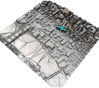
Figure 1: A representation of the stages of urban modeling

2. Data Modelling

2.1.

System Overview and Requirements

For real-time modelling we have some stringent requirements on the types of model. The primary requirement is that the models respect the geometry of the original data but have a good visual appearance. It is desirable for lighting and shadow projection that the building foot-printouts are cut out of the ground plane so that there are no T-junctions on the ground plane. This does mean that a larger number of polygons are required, but it does remove a large number of visual artefacts. We also require that any back-facing or non-visible polygons are removed from the resulting models

2.2.

Partitioning the Ground Plane

We used three principal resources: Ordnance Survey (OS) vector maps, LIDAR (LIght Detection And

Ranging) height data, and aerial photography. In addition we have started to integrate procedures for modelling facades of building.

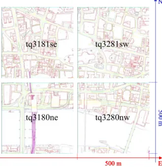
Figure 2 shows four example vector maps from the Land-Line data set. All maps are © Crown Copyright. Land-Line is supplied as tiled data, with each tile comprising 500m x 500m. These are distributed in National Transfer Format (NTF), and we can use either this or the OpenGIS Consortium’s Geography Markup Language (GML).

These maps contain the topography as vector data for both tangible and intangible features. An intangible feature is a map feature that does not represent a real-world object e.g. the line representing a county boundary. The maps contain point data to represent Spot Heights, Triangulation Points etc and line data to represent Building Outlines, Public Road Central Line etc. There is no area type, so areas such as buildings are defined using lines with a unique seed point to identify the area. Feature positions are measured in National Grid coordinates. Features will have a category code denoting their type (Spot Height, Building Outline etc). Features may have an associated text string to indicate the Road Name, House Name, etc.

To satisfy our requirement to uniquely classify the ground plane and to remove ambiguities, we first build a complete Constrained Delaunay Triangulation from the vertices. Delaunay Triangulations are particular triangulations, built on the input data set, which satisfies the empty circum-circle property: the circum-circle of each triangle in the triangulation does not contain any input points. They take in the given input data set and return a structure describing the data set.

Even if OS vector maps sometimes contain errors or ambiguities such as missing edges, using the triangulation and some feature details in the original vector map like buildings’ seeds points and roads’ central lines, we can easily classify the resulting triangles and edges into various sets. For our application we group these in to: Buildings, Pavements, Water and Roads (see Figure 3).

E N 500 m 500 m

tq3180ne

tq3181se

tq3280nw

tq3281sw

tq3180ne

tq3181se

tq3280nw

tq3281sw

2.3. Terrain

Height

At this stage, the model comprises a planar floor. It is suitable for extrusion into a 3D model. This is easily done at this stage, because in the Delaunay Triangulation each vector line has been uniquely attached to two planar triangles, so edges of buildings can be duplicated, one edge raised and the façade polygons inserted. However, if we can obtain height data we have to consider it before extrusion.

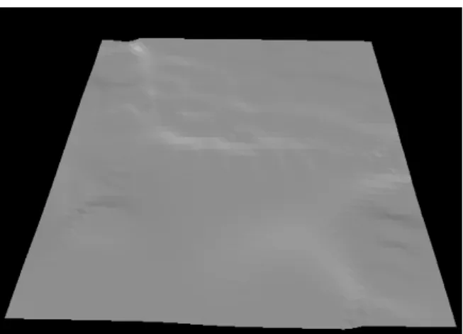
The Land-Line data contains spot heights, but these are too sparse to construct a smooth surface. A better data source, if it is available, is LIDAR. This gives spot heights at densities of typically 30 points per 100 square meters (50 times higher than Land-Line). The horizontal accuracy is 1.5m in the worst case due to uncertainties related to the attitude of the survey aircraft. The vertical accuracy is about +/- 15cm. This data can be used to give both the height of buildings in the previous extrusion step and to construct a terrain height for the ground.

Different methods could be used to create a smooth terrain surface from an unorganised scattered set of data points. The most used techniques are: Kriging and Inverse Distance Weighting (IDW) interpolation. Kriging is a method of interpolation, which predicts unknown values from data observed at known locations. This method uses variogram to express the spatial variation, and it minimizes the error of predicted values, which are estimated by spatial distribution of the predicted values [13]. Kriging is a powerful method; unfortunately the calculations necessary to perform it have a high

computational complexity. Results obtained with the second method (IDW) are comparable with those obtained with Kriging in addition IDW implementation is easier and this algorithm is faster than Kriging. For these reasons we decided to use IDW to find the height of each point on the ground plane. IDW is described in details in Section 3.4. See Figure 4 for an example result.

2.4. Extrusion

Section 2.2 introduced a procedure to find buildings’ outline even in maps containing errors or ambiguities. The basic extrusion algorithm described in this paragraph takes a building outline and extrudes its edges.

The extrusion is done in three parts. Two parts are composed by a ground section, which is one storey high,

Figure 4 Smooth surface created by interpolating the LIDAR data by the inverse distance weighting

function

Figure 5 Triangles comprising a building façade Figure 3 Constrained Delaunay Triangulation

and an upper section, which fills from the 1st _{storey to the}

roof level. These are the pink and green strips in Figure 5. This is done so that a texture map with doors and windows can be used for the ground storey, and with windows only for the upper floors. The extraction procedure must consider the terrain model (see precedent Section) to make more realistic buildings. In effect, the terrain surface normally is not planar, then, individual buildings may not have horizontal edges with the ground. Therefore, a thin polygonal strip is inserted around the base of the building as shown Figure 5 (blue strip). We have chosen to model Buildings with multiple levels so that each level can be textured differently.

At the current time, we are modelling only flat roofs, so to find the height of a building we find the highest LIDAR point within the building footprint, or a close-by but above street-level LIDAR point if the building footprint is small and there is no LIDAR height point within it.

Water features need special treatment, since they will rarely be planar due to surveying and interpolation processes. Water features are flattened by finding their lowest feature point. The water feature is then flattened to this height and appropriate walls put in where the water feature adjoins other features.

2.5.

Other Model Features

If aerial photography exists, then it can be draped over the mesh. We have used sections of the Cities Revealed data set from GeoInformation International for current demonstrations. Since the pixel size of typical aerial photography is around 1 pixel/m, there will be obvious bleeding of ground features to roofs and vice versa.

The Land-Line data contains information about point features such as street furniture and trees. These can be modelled and inserted. Trees are problematic since they also appear on the aerial photography.

Finally pre-modelled buildings can be inserted. This involves some preparation. The original 2D vector data has to be marked so that the polygons are not extruded. So far we have not dealt with fitting the footprint of the pre-modelled building with 2D map, so we simply leave the building outline as a ground plane.

2.6. Other

Outputs

Since we have built a complete Delaunay triangulation of the ground plane, we can robustly classify any new point into a ground coverage type (road, pavement, building, water, etc.). We can use this to create consistent bitmap representations of the model, with, say all buildings classified. This is useful for real-time

collision detection of avatars with models, as demonstrated in the system of Tecchia et al. [17].

From the Delaunay triangulation, we can also construct graphs of road and pavement connectivity by following the mesh connections for a particular ground coverage type. These can be used for path planning for walking or driving simulations. For example, the pavements define walkable surfaces for avatars, and the pavement graph can be used to simplify path searching. In [12] Loscos et al. discuss how to augment the pavement graph network with likely road crossing information so that avatars can walk across the whole map.

3. Air Quality Visualisation

3.1.

Air Quality Information

The pollutant we are studying is carbon monoxide. Transport makes the greatest contribution to carbon monoxide levels and carbon monoxide affects urban areas more significantly than rural areas. Overall carbon monoxide levels have fallen since the 1970s, averaging 1mg/m3 _[4].

The Air Quality Site contains archive data from over 1500 UK monitoring stations going back in some instances to 1972 [2]. Such data sources give a good picture of variation from urban to rural areas. In urban areas some sense of potential variation is conveyed by the difference in readings between kerbside sensors and sensors placed in background areas away from pollutant sources. However they don’t capture the detail of per street variation.

Carbon monoxide disperses over a matter of hours, but Croxford et al. have shown that this is affected by local street configuration [1]. This study used a cluster of sensors in fixed placements in a small area around

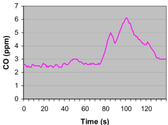
0 1 2 3 4 5 6 7 0 20 40 60 80 100 120 Time (s) CO (ppm)

Figure 6 Raw data from a segment of a path near UCL

University College London (UCL). The Air Quality Strategy for England, Scotland, Wales and Northern Ireland [3], suggests a standard of 10ppm (11.6mg/m3) running 8-hour mean. In the vicinity of UCL, the Croxford study found a peak CO concentration of 12ppm, but nearby sensors reported much lower values near the background level for CO. Thus, moving pedestrians or vehicles would probably not experience this peak for a long period.

3.2. Mapping

Air

Quality

In the Equator IRC e-Science project Advanced Grid Interfaces for Environmental Science in the Lab and in the Field (EPSRC grant GR/R81985/01) [7], we have been investigating ways of mapping pollution using tracked mobile sensors [16]. An accurate carbon monoxide sensor is coupled with a GPS receiver and a logging device. This device can be fitted into a bag or placed on a bike rack. The device logs time, position and pollution level. The resulting recordings are less accurate, but potentially from a wide area of sampling. With several such devices being carried around, it will be possible to build a map that shows detailed local variations in pollution.

3.3.

Raw Pollution Data

The data shown in Figure 6 was collected on a path starting in UCL’s front Quad, and walking up towards Euston Road. Before reaching Euston Road, the user crossed to the other side of the road, and the peak was reached when they were stood near the traffic lights at the junction of Euston Road and Gower St. The peak capture was 6.1 ppm.

3.4. Data

Modelling

The input data for the pollution model is a stream made of a GPS position (xi, yi) and pollution data fi(CO in

parts per million). To make a 2D field representation, we first extract a temporal section of the data. The resulting data set is treated as a set of irregular scatter points.

One of the most commonly used techniques for interpolation of scatter points is Inverse Distance Weighted (IDW) interpolation. IDW methods are based on the assumption that the interpolating surface should be influenced most by the nearby points and less by the more distant points. The interpolating surface is a weighted average of the scatter points and the weight assigned to each scatter point diminishes as the distance from the interpolation point to the scatter point increases.

The simplest form of inverse distance weighted interpolation is Shepard's method [14]. The equation used to find the value at position (x,y) is:

( )

_∑

( )

=

x

y

f

w

y

x

F

,

,

where n is the number of scatter points in the set, fi

are the prescribed function values at the scatter points (e.g. the pollution values), and wi are the weight functions

assigned to each scatter point. The weight function is:

( )

( )

( )

∑

=

y

x

h

y

x

h

y

x

w

,

,

,

where p is a positive real number (typically, p=2) and

( )

(

) (

)

,

i

x

y

x

x

y

y

h

=

−

+

−

The effect of the weight function is that the surface

interpolates each scatter point and is influenced most strongly between scatter points by the points closest to the point being interpolated.

4. Results

4.1. City

Models

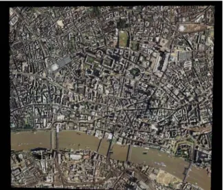
The results of the city model generation are shown in Figures 7 and 8. These show a model of nine sq km around the St Paul’s area of central London. The model comprises 1.2M polygons. Un-optimised this renders at 3-4 frames a second on a PC with GeForce3-4 graphics accelerator. An ongoing theme of research at UCL is interaction and interactive rendering of large-scale urban models [15]. In that demonstration we built a renderer that adapted to frame-rate changes by altering clips volumes and level of detail. The models described in this paper are much superior in detail and geometry to the models used in the previous demonstrator.

4.2. Combined

Data

Our aim in combining data is two fold: to support visualisation by placing the data in the context of the situation where it was gathered, and to support remote collaboration where one participant is using a virtual environment display to collaborate with a colleague in the field. Figure 9 shows views of the junction between Gower St and Euston Road. The blue line represents the recorded path from the GPS receiver. The inaccuracy of GPS location can be noted since the carrier walked along the centre of the pavements except when crossing Gower St.

In the visualisation in Figure 9 we present the pollution interpolation by colouring the roads. In order to maintain a high frame rate, we only interpolate the pollution level at each vertex of the road polygons using the inverse distance weighted interpolation. We then use the built in Gouraud shading algorithm of standard

Figure 9 Views of the junction of Gower St and Euston Road Figure 7 Overview of area around St Paul's

graphics drivers to do a smooth interpolation. This typically uses a bi-linear interpolation. For a more accurate view, a 2D raster image can be calculated at some fixed spatial frequency. In Figure 9 the junction is obviously the most polluted area.

5. Conclusions and Future Work

For the modelling work we are continuing by adding roof structure information. This can be done by determining a roof slopes from LIDAR or by estimating the roof type and then generating a roof that fits [10]. We are also working to integrate better façade texturing that fits with the colour and lighting information from aerial photography. We tend to use either automatic façade texturing or draped aerial photography at the moment since the visual results are often jarring if both are used together. We are also working to integrate Photogrammetric procedures for rapid modelling of specific building facades.

A second activity is on building a run-time that can display larger sections of the virtual model. For ground-level exploration, we can use a combination of occlusion culling and imposter-based rendering. The models we have are very suitable for certain types of occlusion culling, because connectivity between buildings can be recorded and exported.

A third activity is to make a full integration with the crowd animation system of Tecchia, Loscos, et al. [12] [17].

For the pollution modelling we have demonstrated the feasibility of making dense maps of pollution using mobile sensing devices. This enables new types of monitoring that address local variation in pollution and also the levels of pollution that are experienced by different users of the urban space. We hope to establish the pollution monitoring infrastructure as a public infrastructure that can be shared or instantiated by other users.

Further Details

This work is supported by the projects Advanced Grid Interfaces for Environmental e-science in the Lab and in the Field (EPSRC Grant GR/R81985/01) and the EQUATOR Interdisciplinary Research Collaboration (EPSRC Grant GR/N15986/01).

For a complete overview of the environmental e-science project, including a companion project on environmental monitoring in the Antarctic, see the EQUATOR website pages [7]. For example data sets and more detailed specifications of the device see the web page [7]. We plan to make a public release of the software, and to host an example visualisation service at

that address. For further information about the pollution-monitoring project please contact Anthony Steed (A.Steed@cs.ucl.ac.uk).

References

[1] Croxford, B., Penn, A., Hillier, B. (1995) Spatial Distribution of urban pollution: civilizing urban traffic, Fifth Symposium on Highway and Urban Pollution, May 22-24, 1995.

[2] Department for Environment, Food and Rural Affairs (Defra) The Air Quality Archive,

http://www.airquality.co.uk/ (verified 2003-08-13).

[3] Department for Environment, Food and Rural Affairs (Defra) (1999) The Air Quality Strategy for England, Scotland, Wales and Northern Ireland”, 1999, available online at

http://www.defra.gov.uk/environment/consult/airqual ity/pdf/airstrat.pdf (verified 2003-08-13).

[4] Environment Agency, Air Quality – Carbon Monoxide,

http://www.environment-agency.gov.uk/yourenv/eff/air/222825/222913/?lang =_e (verified 2003-08-13).

[5] EQUATOR, Advanced Grid Interfaces for Environmental e-Science: Urban Pollution,

http://www.cs.ucl.ac.uk/research/vr/Projects/envesci/, (verified 2003-08-13).

[6] EQUATOR, City Project,

http://www.dcs.gla.ac.uk/scripts/global/equator/moin. cgi/ (verified 2003-08-13).

[7] EQUATOR, Environmental e-Science Project, http://www.equator.ac.uk/projects/environmental/ind ex.htm (verified 2003-08-13).

[8] EQUATOR, The Equator UnIversal Plaform, http://www.equator.ac.uk/technology/equip/index.ht m (verified 2003-08-13).

[9] Hu, J., You, S., Neumann, U. (2003) Approaches to Large-Scale Urban Modeling, IEEE Computer Graphics and Applications, Nov/Dec,2003

[10] Laycock, R.G. and Day, A.M. (2003). Automatically generating roof models from building footprints, In WSCG, 2003

[11] Learian Design Ltd, http://www.learian.co.uk (verified 2003-08-13)

[12] Loscos, C., Marchal, D., Meyer, A. (2003) Intuitive Crowd Behaviour in Dense Urban Environments using Local Laws, In Theory and Practice of Computer Graphics 2003, IEEE Computer Society Press.

[13] Oliver, M. A. and Webster, R. Kriging: a method of interpolation for geographical information system,

INT. J. Geographical Information Systems, 1990, VOL. 4, No. 3, 313-332

[14] Shepard, D. (1968) A two-dimensional interpolation function for irregularly-spaced data, Proc. 23rd National Conference ACM, ACM, 517-524.

[15] Steed, A., Frecon, E., Pemberton, D., Smith, G. (1999) The London Travel Demonstrator, Proceedings of the ACM Symposium on Virtual Reality Software and Technology, December 20-22nd 1999, pp. 50-57, ACM Press.

[16] Steed, A., Spinello, S., Croxford, B., Greenhalgh, C. (2003). e-Science in the Streets: Urban Pollution Monitoring, UK e-Science All Hands Meeting, September 2003

[17] Tecchia, F., Loscos, C., Chrysanthou, Y. (2002) Visualizing Crowds in Real-Time. Computer Graphics forum, 21(4), December 2002, pages 753-765.