Conditional Narrowing Modulo in Rewriting Logic and Maude

(1)

Conditional Narrowing Modulo in Rewriting

Logic and Maude

Luis Manuel Aguirre Garc´ıa

Máster en Investigación en Informática Facultad de Informática

Universidad Complutense de Madrid

Trabajo de Fin de M´aster en Programaci´on y Tecnolog´ıa Software 9 de septiembre de 2013

Dirigido por: Narciso Mart´ı Oliet Miguel Palomino Tarjuelo Isabel Pita Andreu Convocatoria: Septiembre de 2013

(2)

(3)

Autorizaci´

on de difusi´

on

Luis Manuel Aguirre Garc´ıa

9 de septiembre de 2013

El abajo firmante, matriculado en el Máster en Investigación en Informática de la Facultad de Informática, autoriza a la Universidad Complutense de Madrid (UCM) a difundir y utilizar con fines académicos, no comerciales y mencionando expresamente a su autor el presente trabajo de fin de máster: “Conditional Narrow-ing Modulo in RewritNarrow-ing Logic and Maude”, realizado durante el curso académico 2012-2013 bajo la dirección de Narciso Mart´ı Oliet y Miguel Palomino Tarjuelo, y con la colaboración externa de dirección de Isabel Pita Andreu, en el Depar-tamento de Sistemas Informáticos y Computación, y a la Biblioteca de la UCM a depositarlo en el Archivo Institucional E-Prints Complutense con el objeto de incrementar la difusión, uso e impacto del trabajo en Internet y garantizar su preservación y acceso a largo plazo.

Luis Manuel Aguirre Garc´ıa DNI 00692489-M

(4)

Resumen en castellano

Este trabajo presenta un estudio sobre la resolución de problemas de alcanzabil-idad en teor´ıas de reescritura con una lógica ecuacional de pertenencia subyacente, usando la técnica de estrechamiento. Para ello se han desarrollado dos cálculos, uno que resuelve el problema de unificación módulo la lógica ecuacional y otro que resuelve el problema de alcanzabilidad basándose en el cálculo de unificación pre-vio. Dichos cálculos hacen uso de algoritmos de pertenencia, de unificación módulo axiomas y de encaje, todos ellos disponibles en el lenguaje de reescritura Maude. En ambos cálculos se hace especial énfasis en el uso eficiente de la información sobre los tipos de los términos. Se ha demostrado la corrección y completitud de los cálculos. Posteriormente se han desarrollado sendos conjuntos de reglas de transformación para estos cálculos que permiten la implementación de los mismos. Finalmente, se han programado estas reglas en un prototipo, usando el lenguaje de reescritura Maude.

Palabras clave

Maude, estrechamiento, alcanzabilidad, lógica de reescritura, unificación, lógica ecuacional de pertenencia.

(5)

Abstract

This master’s thesis presents a study about reachability problem solving in rewrite theories with an underlying membership equational logic, using the nar-rowing technique. To achieve this two calculi have been developed , one that solves the unification modulo equational logic problem and another one that solves the reachability problem based on the former unification calculus. Both calculi make use of membership, unification modulo axioms and matching algorithms, all of them available in the rewriting language Maude. Special emphasis has been made on both calculi in the efficient use of term typing information. Soundness and com-pleteness of both calculi has been proved. Afterwards, two sets of transformation rules have been developed to allow the implementation of both calculi. Finally, those rules have been programmed on a prototype, using the rewriting language Maude.

Keywords

Maude, narrowing, reachability, rewriting logic, unification, membership equa-tional logic.

(6)

List of Figures

2.1 Deduction rules for membership equational logic. . . 8 2.2 Deduction rules for rewrite theories. . . 9 2.3 Inference rules for membership rewriting. . . 17

(9)

Chapter 1 Introduction

1.1 Objective

The aim of this work is to study the relationship between verifiable and computable answers toreachability problemsin rewrite theories with an underlying membership equational logic. A reachability problem is an existential formula

(∃x)s(¯¯ x)→∗ t(¯x)

with ¯x some variables, or a conjunction of several of these subgoals.

In this work, a calculus that solves this kind of problems has been developed for rewrite theories. Given a reachability problem in a rewrite theory, this calculus can compute any answer that can be checked by rewriting, or a more general one, one that subsumes the checked one. For instance, instead ofX 7→f(a, b, Z) where Z is a variable,a andb are constants, the calculus may findX 7→f(Y, b, Z) where Y is also a variable. The calculus is first defined for equational unification modulo axioms and its correctness is proven. Then it is extended for reachability goals and also proven correct. The work is not concerned with proving termination in conditional rewriting (see [LMM05] for information on this subject). Special care has been taken in the calculus to keep membership information attached to each term, to make use of it whenever possible (for instance, dropping unfeasible goals or modifying the sort that a term must have depending on the sort of the other term it has to unify with). The calculus does not apply to generalized rewrite theories [BM06] having eitherfrozenarguments [BM06] or context-sensitive strategies [CDE+_{]. We use the rewriting language Maude [}_CDE+₀₂_{] as a tool} for specifying rewrite theories and checking solutions for reachability problems. Some of the functions available on Maude, such as unification modulo axioms or matching modulo axioms, whose algorithms are very complex [HM12], are used in the calculus.

(10)

2 1.2. Motivation

1.2 Motivation

Since the late 60’s there has been a concern in the programming community about the semantics of programs. The increasing complexity of computer programs made necessary the development of languages, tools and mathematical methods that could improve the speed and safety when developing programs. One of the first milestones was Tony Hoare’s axiomatic semantics [Hoa69]. In the following twenty years there were several proposals of languages, such as OBJ3 [GKK+87], and models for concurrent system specification, such as Petri nets [Pet73] or CCS [Mil80].

Rewriting logic is a computational logic that has been around for more than twenty years [Mes90], whose semantics [BM06] has a precise mathematical meaning allowing mathematical reasoning for property proving, as an attempt to provide a more flexible framework for the specification of concurrent systems. It turned out that it can express both concurrent computation and logical deduction, allowing its application in many areas such as automated deduction, software and hardware specification and verification, security, etc.

On the computational side, rewriting logic is a semantic framework that al-lows natural representation, execution and analysis as rewrite theories of different concurrency models, distributed algorithms, etc. On the logic side, it is a logi-cal framework that allows representation and reasoning about different logics and automated decision procedures.

One important property of rewriting logic is that the distance between the represented structure and its representation in rewriting logic is very small. Usually they are isomorphic structures where differences are due to the notations used on both sides, but the main features remain the same. This allows reducing errors when coding.

Another important property of rewriting logic is reflection [CM96]. Intuitively, reflection means representing a logic’s metalevel at the object level, allowing the definition of strategies that guide rule application in an object-level theory. A classic example of reflection can be found on Turing’s Universal Machine [Tur36]. The reachability problem can be solved by model checking methods [CGP99] for finite state spaces. A technique known as narrowing [Fay78] that was first proposed as a method for solving equational goals (unification), has been extended to cover also reachability goals [DMT98], leaving equational goals as a special case of reachability goals. This technique resembles symbolic model checking, where we represent infinite sets of states using logical variables in terms. Variables get instantiated through the narrowing process, when necessary. In recent years the idea ofvariants of term [CLD05] has been applied to narrowing. The variants of a terms are pairs (t, θ), meaning that termsrewrites to the irreducible (canonical) term t using substitution θ. A strategy for order-sorted unconditional rewrite

(11)

1. Introduction 3

theories known as folding variant narrowing [ESM12], which computes a complete set of variants of any termS, has been developed by Escobar, Sasse and Meseguer, allowing unificationmodulo a set of equations and axioms. The strategy terminates on any input term on those systems enjoying the finite variant property [CLD05], a characterization that ensures that any term has a finite number of variants, and it is optimally terminating, that is, if any complete narrowing strategy terminates on an input term, the folding variant narrowing will terminate on this term. It is being used for cryptographic protocol analysis [MT07], with tools like Maude-NPA [EMM05], termination algorithms modulo axioms [DLM09], and algorithms for checking confluence and coherence of rewrite theories modulo axioms, such as the Church-Rosser (CRC) and the Coherence (ChC) Checkers for Maude [DM12]. This work explores narrowing for membership conditional rewrite theories, go-ing beyond the scope of foldgo-ing variant narrowgo-ing which works on order-sorted unconditional rewrite theories. A calculus that computes answers to reachabil-ity problems in membership conditional rewrite theories has been developed and proved correct with respect to idempotent normalized answers, that is, given a solution for a reachability problem the calculus can compute one answer that sub-sumes (includes) this solution, and if the calculus computes one answer then the answer is a solution for the reachability problem.

1.3 Structure of the work

• In Chapter2all needed definitions and properties for rewriting and narrowing are introduced.

• Chapter 3 is a brief introduction to the rewriting language Maude, empha-sizing the needed parts of it.

• Chapter 4 introduces the first part of the narrowing calculus, the one that deals with equational unification. In this calculus the rule to apply each time is always correctly chosen (we have an oracle). All we show is that an answer exists (if it does). We are not concerned on how to choose rules (this is a strategy). There are several examples showing the calculus at work.

• In Chapter 5 the proofs of soundness and completeness of the calculus for unification presented in Chapter 4 are shown.

• In Chapter 6 a set of transformations for the previous calculus is presented. An example shows the inner working of this set of transformations.

• Chapter 7 introduces the rest of the calculus, the part dealing with reacha-bility. Again, we have an oracle that always guesses the right rule to apply.

(12)

4 1.3. Structure of the work

• Chapter8holds the proofs of soundness and completeness of the calculus for reachability presented in Chapter7.

• In Chapter9a set of transformations for the rest of the calculus is presented. Another example shows the inner working of this set of transformations. It is worth pointing out that the whole set of transformations work at the metalevel, with the given rewrite theory as an object. This is where possible enhancements can be made via strategies.

• Chapter10discusses the implementation of the set of transformations, struc-ture and flow control, together with improvements that can be made at this stage. Source code for the implementation, as well as several examples and in-structions for its use can be found inhttp://maude.sip.ucm.es/cnarrowing/.

• In Chapter11, conclusions and further improvements and lines of investiga-tion for this work are presented.

(13)

Chapter 2 Preliminaries

Rewriting logic, as it has been said, is a general logical framework in which many deductive systems can be naturally represented [BM06]. There are several language implementations of rewriting logic, including Maude [CDE+₀₂_{]. Rewriting logic} is parameterized by an underlying equational logic. In Maude’s case this logic is membership equational logic [Mes97].

In this Section we introduce the equational part of the logic, then the rewrite part of it. We follow by presenting sufficient conditions under which these logics are computable. Then unification, the problem of assigning values to variables in terms to make them equationally equal, is described. The equivalent problem for rewriting (reachability) is presented, and a technique (narrowing) that suits both problems is described. We end the Section showing a transformation that turns a unification problem into a reachability one, allowing us to solve both kinds of problems using the same techniques.

Throughout this Section a theoretical vending machine (what else!) will be used as a motivating example to explain the definitions in an less abstract way. This machine accepts a Coin(a quarter (q) or a dollar ($), as it is U.S. made) that may be inserted at any time, and nondeterministically serves one Item if there is enough credit: an apple (a) at a price of one dollar, or a coffee (c) at a price of three quarters. The vending machine is rather odd: in order to serve a coffee there must be a credit of at least a whole dollar; then the machine may serve the coffee (or an apple). The vending machine knows that four quarters make a dollar. If there is a credit of three quarters, the machine serves nothing (although it has enough money to serve a coffee). As there must always be a credit of a whole dollar before the vending machine serves anything, we never know if we are going to get a coffee or an apple. The vending machine has aStatewhich is a nonempty multiset of Coins and Items (the initial State may not be empty). The State

tells us the credit, and theItems that have already been served. A singleCoin or

Item is aState. States are written as a mere juxtaposition of Coinsand Items, 5

(14)

6 2.1. Membership equational logic

that is, we use an empty operator. Parentheses may be used to enclose several items of aState if desired.

2.1 Membership equational logic

We first describe the static (equational) part of our theories. This includes the items we are going to work with (operators, terms, kinds, sorts, etc) as well as the criteria to consider that two syntactically different terms belong to the same class of terms (conditional equations and memberships), that is, we define equivalence classes on terms. We also define essential concepts, like positions or substitutions, which will be widely used.

Amembership equational logic(_Mel)signature[BM06] is a triple Σ = (K,Ω, S), with K a set of kinds, Ω = {Σw,k}(w,k)∈K∗_x_K a many-kinded algebraic signature,

and S = {Sk}k∈K a K-kinded family of disjoint sets of sorts. The kind of a sort s is denoted by [s]. The sets TΣ,s, TΣ(X)s, TΣ,k and TΣ(X)k denote, respectively, the set of ground Σ-terms with sort s, the set of Σ-terms with sort s over the set X of sorted variables, the set of ground Σ-terms with kind k and the set of Σ-terms with kind k over the setX of sorted variables. We write TΣ, TΣ(X) for

the corresponding term algebras. Given a term t ∈ TΣ(X), the set vars(t) ⊆ X

denotes the set of variables int.

The Mel signature (Σ) for our vending machine has only one kind, K = {[State]}, with three sorts, S[State] = {State,Coin,Item}. S = {S[State]}. Ω =

{·[State] [State],[State]}, that is there is only one function (·, understood as

juxtapo-sition) that given a pair of elements with kind [State] returns another element with kind[State]. TΣ,Coin ={q,$}, TΣ,Item ={a,c}. q, $, a and c are theatoms

(oratomic values) of our signature. Any ground term has to be either one of these atoms or some term made up with these atoms and the only constructor operator

(·).

When a term t is parsed as a tree, the empty string represents the root of t. Positions in a term t are denoted as strings of nonzero natural numbers and represent nodes or leaves of its parsed tree. The set of positions of a term is written Pos(t), and the set of non-variable positions PosΣ(t). If we consider the

subtree of t below a certain position p, p being the root of the subtree, we get a subterm of the term t denoted by t|p. For instance the subterm at position 2 of t ≡ f(a, g(b, c)) is t|2 ≡ g(b, c). The replacement in t of a subterm at position p

by another termu is denoted by t[u]p.

Asubstitution σ :Y →TΣ(X) is a function from a finite set of sorted variables

Y ⊆X toTΣ(X) such thatσ(y) has the same or lower sort as that of the variable

y ∈ Y (s1 ≤ s2, formally defined in the next paragraph). The application of a

(15)

2. Preliminaries 7

tis a term obtained from tbysimultaneously replacing each occurrence of variable y∈Dom(σ) intwith σ(y). Substitutions are written asσ={X1 7→t1, . . . , Xn7→ tn} where the domain of σ is Dom(σ) = {X1, . . . , Xn} and the set of variables introduced by terms t1, . . . , tn is written Ran(σ). The identity substitution is id. Substitutions σ : Y → TΣ(X) are homomorphically extended to TΣ(X), written

with the same notation σ : TΣ(X) → TΣ(X). For simplicity, we assume that

every substitution is idempotent,that is, σ satisfies Dom(σ)∩Ran(σ) = ∅. The restriction of σ to a set of variables V is σ|V; sometimes we write σ|t1,...,tn to

denote σ|V where V =Var(t1), . . . ,Var(tn). Composition of two substitutions is denoted by σσ0. Combination of two substitutions is denoted by σ∪σ0. We call an idempotent substitution σ a variable renaming if there is another idempotent substitution σ−1 _{such that (σσ}−1₎_|

Dom(σ) =id.

In our vending machine, if t = qXItem and σ = {XItem 7→ c} then tσ = qc,

which is a term with sort State, as we will now see.

A _Mel theory [BM06] is a pair (Σ,E), where Σ is a _Mel signature and E

is a finite set of Mel sentences, either a conditional equation or a conditional

membership of the forms:

(∀X) t=t0 if ^

i

Ai, (∀X)t:s if ^

i Ai

fort, t0 ∈TΣ(X)k and s∈Sk, the latter stating thatt is a term of sorts, provided the condition holds, and each Ai can be of the form t=t0, t:s or t:=t0 (a matching equation). Matching equations are treated as ordinary equations, but they impose a limitation in the syntax of admissible Mel theories, as we will see.

Order-sorted notation s1 ≤s2 can be used instead of (∀x:[s1]) x:s2 if x:s1. An operator

declaration f :s1× · · · ×sn →s corresponds to declaring f at the kind level and giving the membership axiom (∀x1:k1, . . . , xn:kn) f(x1, . . . , xn):s if

V

1≤i≤nxi:si. Given a Melsentence φ, we denote byE `φ that φcan be deduced from E using

the rules in Figure 2.1, where = can be either = or := as explained before [BM12]. The Mel theory for our vending machine consists of the Mel signature Σ

defined before, and the following set E of Mel sentences:

• ∀X:[State] X:State if X:Item(every Item is a State, or Item≤State)

• ∀X:[State] X:State if X:Coin(every Coin is a State, or Coin≤State)

• ∀X, Y:[State] XY:State if X:State ∧ Y:State

(the juxtaposition of States is a State)

• ∀X, Y:[State] XY =Y X (juxtaposition is commutative)

(16)

8 2.2. Rewriting logic t∈TΣ(X) (∀X)t=t Reflexivity (∀X)t=t0 (∀X)t0₌_t Symmetry (∀X)t1=t2 (∀X)t2=t3 (∀X)t1=t3 Transitivity (∀X)t0:s (∀X)t=t0 (∀X)t:s Membership f ∈Σk1···kn,k (∀X)ti=t 0 i ti, t0i∈TΣ(X)ki,1≤i≤n (∀X)f(t1, . . . , tn) =f(t01, . . . , t0n) Congruence ((∀X)A0if ViAi)∈E θ:X→TΣ(Y) (∀Y)Aiθ (∀Y)A0θ Replacement

Figure 2.1: Deduction rules for membership equational logic.

• qqqq= $ (four quarters make a dollar)

A Σ-algebra A [Mes97] consists of a set Ak for each kind k, a function Af : Ak1x· · ·xAkn for each operator f ∈ Σk1···kn,k, and a subset inclusion As ⊆ Ak for

each sorts∈Sk. For a valuationa:X →Aassigning a value inAsto each variable x∈Xwith sorts, if ¯a:TΣ(X)→Ais the homomorphic extension ofato terms, by

definition, A, a |= (∀X)t = t0 iff ¯a(t) = ¯a(t0), and A, a |= (∀X)t : s iff ¯a(t)∈ As. A Σ-algebra A is a model of a formula φ, written A |= φ, when φ is satisfied for any valuationa. A Mel sentence ϕis a logical consequence of (Σ,E), written

(Σ,E)|=ϕ, when all the models of (Σ,E) are also models ofϕ. The rules of Figure 2.1 specify a sound and complete calculus, that is, (Σ,E) ` ϕ ⇐⇒ (Σ,E) |= ϕ. A Mel theory (Σ,E) has an initial algebra, denoted by TΣ/E, whose elements are

equivalence classes [t]E ⊆TΣ of ground terms identified by the equations in E.

The initial algebra for the vending machine is the set of all non-empty multisets that can be made up with the four atoms q, $, c, a. Recall that, for instance

{a, a, q} and {a, q, a} are the same multiset, but they are not the multiset{a, q}.

2.2 Rewriting logic

Now we describe the dynamic part of our theories. These are the conditional rewrite rules that make our system evolve, be it a concurrent or a deductive system. A rewrite theory R = (Σ,E, R) is a formal specification of concurrent or de-ductive systems [Mes92], where

• (Σ,E) is a theory in membership equational logic

• R is a finite set of labeled conditional rewrite rules, each of which has the form (= can be either = or :=):

λ: (∀X)l →r if ^ i pi=qi∧ ^ j wj:sj∧ ^ k lk→rk,

(17)

2. Preliminaries 9 t∈TΣ(X) (∀X)t→t Reflexivity (∀X)t1→t2, (∀X)t2→t3 (∀X)t1→t3 Transitivity (∀X)u→u0_, _{E `}_(∀_X₎_t₌_u, _{E `}_(∀_X₎_u0₌_t0 (∀X)t→t0 Equality f ∈Σk1···kn,k (∀X)ti →t 0 i ti, t0i∈TΣ(X)ki,1≤i≤n (∀X)f(t1, . . . , tn)→f(t01, . . . , t0n) Congruence (λ: (∀X)l→rif^ i pi=qi∧ ^ j wj:sj∧ ^ k lk→rk)∈R θ:X→TΣ(Y) ViE `(∀Y)piθ=qiθ VjE `(∀Y)wjθ:sj Vk(∀Y)lkθ→rkθ (∀Y)lθ→rθ Replacement

Figure 2.2: Deduction rules for rewrite theories.

Such a rewrite rule specifies aone-step transition (often called aone-step rewrite) from a statet[lθ]p containing a substitution instancelθ at a positionpto the state t[rθ]p in whichlθ has been replaced by the corresponding instance rθ, denoted by t[lθ]p →1

Rt[rθ]p, provided the condition holds; that is, the substitution instance by θ of each condition in the rule follows fromR. The subterm t|p is called a redex.

In our vending machine, R is the following set of labeled conditional rewrite rules:

• add-quarter: ∀X:[State] X→Xq if X:State (quarter inserted)

• add-dollar: ∀X:[State]X →X$ if X:State (dollar inserted)

• buy-coffee: $→c (coffee served)

• buy-apple: $→aq (apple served, credit updated)

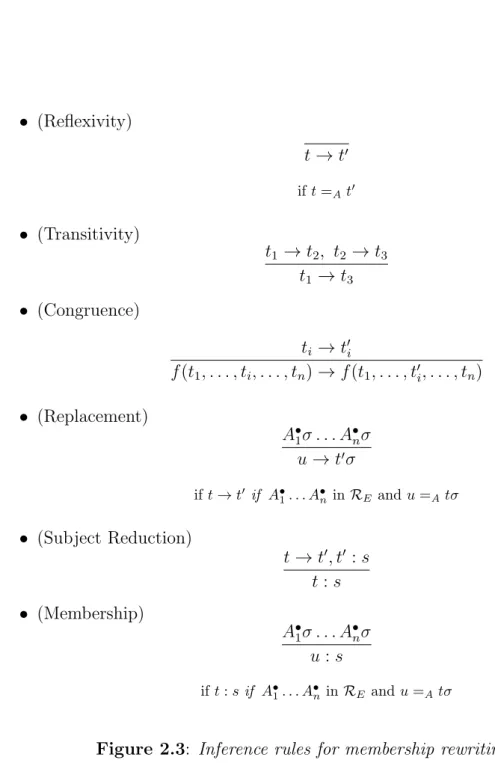
The inference rules [BM12] in Figure 2.2 for rewrite theories can infer all pos-sible deductive computations in the system specified by R. We can reach a state v from a state u if we can prove R `u→v.

The relation →1

R/E on TΣ(X) is =E ◦ →1R ◦ =E. →1_R/E on TΣ(X) induces a

relation →1

R/E on TΣ/E(X), the equivalence relation modulo E, by [t]E →1_R/E [t 0_]

E

iff t →1

R/E t

0_{. The transitive (resp. transitive and reflexive) closure of} _→1

R/E is

denoted →+

R/E (resp. → ∗

R/E). We say that a term t is →R/E-irreducible (or just

R/E-irreducible) if there is no termt0 such that t→1

R/E t 0_.

We define now several properties that rewrite rules, rewrite theories substitu-tions or relasubstitu-tions may have. It is not mandatory for all rewrite theories to have

(18)

10 2.3. Executable rewrite theories

all properties, but some of them will be required to make the rewrite theories computable.

For a rewrite rule l → r if cond, we say that it is sort-decreasing if for each substitution σ, we have that rσ ∈ TΣ(X)s and (cond)σ is verified implies lσ∈TΣ(X)s, that is, if we apply this rule to a termt with sorts, we get anothert0 whose sorts0 is lower than or equal tos. We say that a rewrite theoryR= (Σ,E, R) is sort-decreasing if all rules in R are. For a Σ-equation t = t0, we say that it is

regular if Var(t) = Var(t0), that is, there are no extra variables, and it is sort-preserving if for each substitution σ, we have tσ ∈ Tσ(X)s implies t0σ ∈ Tσ(X)s and vice versa. We say a rewrite theoryR= (Σ,E, R) is regular or sort-preserving if all equations inE are.

For substitutions σ, ρ and a set of variablesV we define σ|V →1_R/E ρ|V if there isx ∈V such thatσ(x)→1

R/E ρ(x) and for all other y ∈V we haveσ(y) =E ρ(y).

A substitution is called E-normalized (or normalized) if xσ is E-irreducible for all x∈V. This is the simplest version moduloE for that substitution.

We say that the relation →1

R/E is terminating if there is no infinite sequence

t1 →1_R/E t2 →1_R/E · · ·tn→1_R/E tn+1· · ·. We say that the relation →1_R/E is confluent

if whenever t →∗

R/E t

0 _and _t _→∗

R/E t

00_{, there exists a term} _t000 _{such that} _t0 _→∗

R/E t 000

and t00 →∗

R/E t

000_{. A rewrite theory} _R _{= (Σ,}_E_{, R) is confluent (resp. terminating)}

if the relation →1

R/E is confluent (resp. terminating). In a confluent, terminating,

sort-decreasing, membership rewrite theory, for each term t ∈ TΣ(X), there is

a unique (up to E-equivalence) R/E-irreducible term t0 obtained by rewriting to

canonical form, denoted byt →!

R/E t0, ort ↓R/E when t0 is not relevant, which we

callcanR/E(t). Then, we can apply any available rule each time, and obtain always

the same canonical form modulo E. We write t ↓ or can(t) when the underlying rewriting logic is known.

Our vending machine is, as most reactive systems are [AILS07], non termi-nating. From any initial State we can always apply rules add-quarter and

add-dollar. Rule buy-coffee is not sort-decreasing because it can turn a term with sortCoininto a term with sortItem, and it is not true thatItem≤Coin. Also rule buy-apple is not sort-decreasing because it can turn a term with sort Coin

into a term with sortState, which is strictly bigger than sortCoin(Coin≤State

and StateCoin.)

2.3 Executable rewrite theories

For a rewrite theory R = (Σ,E, R), whether a one step rewrite t →1

R/E t

0 _holds

is undecidable in general. We impose additional conditions under which we can computationally decide ift→1

R/E t

(19)

2. Preliminaries 11

and, in fact, they allow a great number of systems to be specified. We decompose

E =E∪A. A rewrite theory R = (Σ, E∪A, R) is executable if each kind k in Σ is nonempty, E, A, and R are finite and the following conditions hold:

1. E and R are admissible, that is, the set E consists of conditional equations (1) and conditional memberships (2), and the set R consists of conditional rules (3), where in (1) the variables in t0 are among those in t or in some Ai, and where, in (1), (2) and (3) each Ai can be either a membership ti:si, equation ti=t0_i or matching equation ti:=t0_i such that any new variable not in t or in some Aj with j < i must occur only in ti or in some Aj with j > i; furthermore, ifti introduces any new variables, then ti must be a non variable term. In (3), given a conditional rule of the form

l :t→t0 if A1∧. . .∧An,

Ai can also be a rewriteti →t0i. Then it must satisfy the additional require-ment vars(ti)⊆vars(t)∪ i−1 [ j=1 vars(Aj),

and furthermore t0_i is an E-pattern1_{. Logically we treat matching equations}

as ordinary equations. The point with admissible theories is that they allow us to assign values to new variables by matching. With the conditions for a matching equation, its left side is an E-pattern, and can not be rewritten, so we rewrite the right side of the matching equation to canonical form and match it against the new variables in the left side.

2. Equality modulo A, i.e., t =A t0, is decidable and there exists a matching

algorithm modulo A, producing a finite number ofA-matching substitutions or failing otherwise, that can implement rewriting in A-equivalence classes. Usually, Aare axioms of commutativity, associativity and identity that may be non terminating under standard rewriting. We put these axioms apart from the terminating ones and use special algorithms for them, that are designed to avoid non terminating behaviors.

3. The equationsE are sort-decreasing, andterminating, coherent, and conflu-ent modulo Awhen we consider them as oriented rules. Sort-decreasingness,

1_{We call a term}_t_an_E_{-pattern if for any well-formed substitution}_σ_{such that for each variable}

xin its domain the termσ(x) is in canonical form with respect to the equations inE, thentσis also in canonical form. A sufficient condition for tto be anE-pattern is the absence of unifiers (see2.4) between its non variable subterms and left hand sides of equations inE. There is recent work on this kind of unification where one term is always in normal form so no rewrite rules can ever be applied to it, which has been calledasymmetric unification [EEK+₁₃_]

(20)

12 2.4. Unification

confluence and termination allow us to represent E-equivalence classes as A-equivalence classes in E/A-canonical form uniquely. The A-coherence as-sumption makes it possible to compute the rewrite relation →1

E/A on A-equivalence classes by means of an A-matching algorithm.

4. The rules R are coherent relative to the equations E modulo A. That is, together with the above conditions, if t is rewritten to t0 by a rule (l →

r if cond), the E-canonical term canE/A(t) is also rewritten to t00 by the

same rule such thatcanE/A(t0) =A canE/A(t00). Technically, what coherence means is that the weaker relation →1

E,A (defined in the last paragraph of this Section) becomes semantically equivalent to the stronger relation→1

E/A, so we can decide t →1

R/E t

0 _{by finding} _t00 _{such that} _can

E,A(t) →1R t

00 _and

canE,A(t0) =A canE,A(t00), which is a decidable, since the number of rules is finite and A-matching is decidable.

The rewrite theory for our vending machine is executable if we decompose E

in the following way: the setA has as elements the equations for the commutative and the associative properties for function·(juxtaposition), the setEhas the other equation and all memberships. E and R are admissible because they are regular and don’t introduce new variables. A has a matching algorithm (when we use Maude it is calledmatch). The equations E are sort-decreasing, andterminating, coherent, and confluent modulo A when we consider them as oriented rules and the rules R are coherent relative to the equations E modulo A. We will not go further into these properties, that must be checked by the user, but Maude provides tools like the Church-Rosser (CRC) and the Coherence (ChC) Checkers for Maude [DM12] that help the user verify them.

For executable rewrite theories R = (Σ,E, R) with E = E∪A we define the relation→1

E,A onTΣ(X) as follows: t →1E,A t

0 _{if there is an} _ω_∈_Pos_(t),_l ₌_r_∈_E,

and a substitution σ such that t|w =A lσ (A-matching) and t0 = t[rσ]ω. Since A is sort-preserving and E is sort-decreasing, t0 is well-sorted, that is t ∈ TΣ(X)s

implies t0 ∈ TΣ(X)s. The relation →1R,A is similarly defined, and because of our assumption about the signature Σ, it is the case that t →1

R,A t

0 _implies _t0 _is

well-sorted, andt∈TΣ(X)[s]impliest0 ∈TΣ(X)[s]. We define→1R∪E,A as→1R,A∪ →1E,A. Note that, sinceA-matching is decidable,→1

E,A, →1R,A, and→1R∪E,A are decidable. These three relations are lifted to substitutions as expected. R∪E, A-normalized (and similarlyR, A orE, A-normalized) substitutions are defined as expected.

2.4 Unification

Unification tries to assign values to variables in two terms t and t0 through a substitution σ in a way such that they become syntactically equal (tσ =E t0σ)

(21)

2. Preliminaries 13

[Baa90]. In membership equational logic we answer the question∀(¯x)t(¯x)=t0(¯x)? In unification we answer the question ∃(¯x)t(¯x)=t0(¯x)?

For instance, the membership equational logic for the vending machine tells us that ifX is a variable with sortState thenXqqqq =X$ whatever X is, but with unification we know that Xqqq= $ only if we use the substitution {X 7→q}.

Given an executable rewrite theoryR= (Σ,E, R), a Σ-equationis an expression of the form t = t0 where t, t0 ∈ TΣ(X)s for an appropriate s. The E-subsumption

preorderE onTΣ(X)sis defined bytE t0 (meaning thatt0 is more general than

t) if there is a substitution σ such thatt =E t0σ; such a substitutionσ is said to be

Asystem of equations F is a conjunction of the formt1 =t01∧. . .∧tn =t0nwhere for 1 ≤ i ≤ n, ti =t0i is a Σ-equation. We define Var(F) =

S

iVar(ti)∪Var(t0i). An E-unifier for F is a substitution σ such that tiσ =E t0iσ for 1≤ i ≤n. When

E = ∅ (no associativity, no commutativity, etc.) there is at much one unifier. In the general case, the set of unifiers for a system of equations may not be finite. ForV =Var(F)⊆W, a set of substitutions CSUE(F, W) is said to be acomplete

set of unifiers of F away fromW [GS89] if

• each σ∈CSUE(F, W) is an E-unifier of F;

• for any E-unifier ρof F there is a σ ∈CSUE(F, W) such that ρ|V E σ|V;

• for all σ ∈CSUE(F, W), Dom(σ)⊆V and Ran(σ)∩W =∅.

That is, a complete set of unifiers CSUE(F, W) is composed of idempotent

E-unifiers of F such that they only instantiate variables on F, no new variable on the unifiers belongs to the setW, and for any other E-unifier of F there is a more general one in CSUE(F, W) with respect to the variables inF.

An E-unification algorithm is complete if for any given system of equations it generates a complete set of E-unifiers, which may not be finite. A unification algorithm is said to be finite and complete if it terminates after generating a finite and complete set of solutions.

Checking if ρ is an E-unifier of F is achieved by E, A-rewriting. Using the equations in E as oriented rules and the matching algorithm for A we rewrite the terms inF to canonical form and check if each left side canonical termcanE/A(tiρ) is equal moduloA(we use the matching algorithm) to the corresponding right side canonical term canE/A(t0iρ).

(22)

14 2.5. Reachability goals

2.5 Reachability goals

Reachability goals and their solving are the main subjects of this work. We first define reachability goals, then we define solutions and trivial solutions of them. We follow by characterizing the needed properties in our rewrite theories that makes us able to compute solutions of reachability problems.

Given a rewrite theory R = (Σ,E, R), a reachability goal G is a conjunction of the form t1 →∗ t01 ∧. . .∧tn →∗ tn0 where for 1 ≤ i ≤ n, ti, t0i ∈ TΣ(X)si for

appropriate si. We say that ti are the sources of the goal G, while t0i are the

targets. We define Var(G) = S

iVar(ti)∪Var(t0i). A substitution σ is a solution of G if tiσ →∗_R/E t

0

iσ for 1≤i≤n. We define E(G) to be the system of equations t1 =t01∧. . .∧tn =t0n. We say σ is a trivial solution of G if it is an E-unifier for E(G). We say G is trivial if the identity substitution id is a trivial solution of G. For instance, in the rewrite theory for the vending machine if X is a variable with sort State, then {X 7→ q} is a trivial solution of the reachability goal G ≡

Xqqq → $, but it is a non-trivial solution of the reachability goal G≡ Xqq → $

(qqq→add−quarter qqqq →equality $).

For goals G:t1 →∗ t2∧. . .∧t2n−1 →∗ t2nand G0 :t01 →

∗ _t0 2∧. . .∧t 0 2n−1 → ∗ _t0 2n we say G =E G0 if ti =E t0i for 1 ≤ i ≤ 2n. We say G →R G0 if there is an odd i such that ti →R t0i and for all j 6= i we have tj = t

0

j. That is, G and G

0

differ only in one subgoal (ti →ti+1 vs t0i →ti+1), but ti →t0i, so when we rewrite ti in G to t0_i we get G0. We write G →r,R G0 meaning that rule r ∈ R has been used in the rewriting step from G to G0. The relation →R/E over goals is defined as

=E ◦ →R◦=E.

We implement →R/E (on terms and goals) using →R∪E,A [MT07]. This lemma links →R/E with →E,A and →R,A. Patrick Viry gave a proof for unsorted uncon-ditional rewrite theories [Vir94], which can easily be applied to our membership conditional case [MT07].

LemmaLet R= (Σ,E, R) be an executable rewrite theory, that is, it has all the properties specified in Section 2.3. Thent1 →R/E t2 if and only if t1 →∗E,A→R,At3

for some t3 =E t2.

Thus t1 →∗_R/E t2 if and only if t1 →∗R∪E,A t3 for some t3 =E t2, which can be

decided by checkingt3↓E,A=At2↓E,A with the A-matching algorithm. This is the way rewriting is decided: from termt1we compute its derivation tree in a

breadth-first way and check each resulting term againstt2 with theA-matching algorithm.

If some term matches then the rewriting is possible and we have found a proof for it. This result is lifted to goals as G1 →∗R/E G2 if and only if G1 →∗R∪E,A G3 for

some G3 =E G2. Also, σ is a trivial solution of t1=t01∧. . .∧tn=t0n if and only if t1σ↓E,A =At01σ↓E,A∧. . .∧tnσ↓E,A =A t0nσ↓E,A.

(23)

2. Preliminaries 15

2.6 Narrowing

Narrowing is like rewriting, but replacing matching modulo an equational theory with unification modulo that theory. It tries to assign values to variables in two terms t and t0 through a substitution σ in a way such that tσ →R/E t0σ (see

[KK96, Ch. 14, p. 181-190] for a full description). In rewriting logic we answer the question∀(¯x)t(¯x)→t0(¯x)? In narrowing we answer the question∃(¯x)t(¯x)→t0(¯x)?. Unification is the only allowed way to assigns values, ground or not, to variables in narrowing. We don’t guess values, we unify two terms modulo the given equational theory and use the resulting substitution as a partial or total answer.

In the vending machine example we can prove by rewriting that for a variable X with sort State X$ → Xc whatever value X is given. Finding out that the substitution {X 7→ q} is a solution of the reachability goal Xqqq → c requires narrowing.

Let t be a Σ-term and W be a set of variables such that Var(t) ⊆ W. The R, A-narrowing relation on TΣ(X) is defined as follows: t p,σ,R,A t0 if there is a non-variable position p ∈PosΣ(t), a rulel → r if cond in R, properly renamed,

such thatVar(l)∩W =∅, and a unifier σ ∈CSU_AW0(t|p =l) forW0 =W∪Var(l), such that t0 = (t[r]p)σ and (cond)σ holds. This is lifted to reachability goals as follows. LetG:t1 →∗ t2∧. . .∧t2n−1 →∗ t2n andG0 :t01 →∗ t02∧. . .∧t02n−1 →∗ t02n, and suppose that Var(G) ⊆ V. We define G σ,R,A G0 if there is an odd i such that ti p,σ,R,At0i for some σ that is away from Var(G), and for all j 6=i we have t0_j =tjσ. We writeG ∗σ,R,A G0 if eitherG=G0 and σ=id, or there is a sequence of derivations G σ1,R,A . . . σn,R,A G

0 _{such that} _σ ₌ _σ

1. . . σn. Similarly E, A-narrowing and R ∪E, A-narrowing relations are defined on terms and goals, as expected.

Back to our vending machine and the reachability goal Xqqq → c, we have that (Xqqq)σ ≡ qqqq ,σ,R∪E,A $ ≡ ($)σ using the oriented equation qqqq = $ as a rule and unifier σ={X 7→ q} ∈ CSU_AW0(Xqqq| = qqqq), and $ ,id,R∪E,A c using rule buy-coffee: $→c, so it takes two narrowing steps, one with an oriented equation and another one with a rule, to find the answer.

2.7 Unification by rewriting

We have defined unification, but we have not given a method to compute unifiers. In this Section we show an equivalent definition for executable Mel theories that

makes this computation possible. Furthermore, our calculus will make use of this equivalence to intermix both rewritings, for unification and reachability, instead of carrying an independent computation with each one.

(24)

16 2.7. Unification by rewriting

2.7.1 Associated rewrite theory

Any executable_Mel theory (Σ, E∪A) has a corresponding rewrite theoryRE = (Σ0,A∪ME, RE) associated to it, defined in [DLM+08, Ch. 3, p. 10-13], that allows us to check if a substitutionσ is a solution for a goal Gthrough rewriting instead of equational unification. We will use either of these approaches when proving properties of the calculus. It is defined in [DLM+₀₈_{] as follows: we add a fresh} new kind Truth with a constant tt to Σ, and for each kind k ∈ K an operator

eq : k k → Truth. We write > to represent a conjunction of any number of tt’s. The equational axioms are the ones in A. There are rules eq(x:k, x:k) → tt for each kind k ∈K. Furthermore, for each admissible conditional equation inE the setRE has a conditional rule of the form

t→t0 if A•₁∧. . .∧A•_n

where ifAi is a membership then A•_i=Ai, ifAi is a matching equation ti:=t0_i then A•_i is the rewrite conditiont0_i→ti, and ifAi is an ordinary equationt=t0 thenA•i is the rewrite condition eq(t, t0)→tt. Similarly, for each conditional membership in E we add toME a conditional membership, withA•_i as before, of the form,

t:s if A•₁∧. . .∧A•_n Systems of equations in (Σ, E∪A) with form G≡ Vm

i=1(si =ti) become reacha-bility goals in RE with formVm_i₌₁eq(si, ti)→tt. A substitution σ is a solution of Gif there are derivations for Vm

i=1(siσ =tiσ), or

Vm

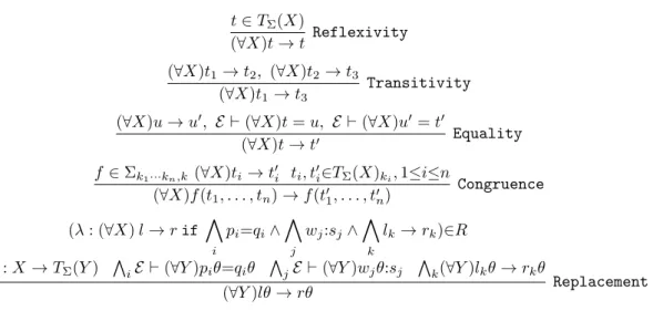
i=1eq(siσ, tiσ) rewrites to >. The inference rules for membership rewriting in RE are the ones in Figure 2.3, adapted from [DLM+₀₈_{, Fig. 4, p. 12], where the rules are defined for} context-sensitive membership rewriting.

2.7.2 Computing

E

-unifiers

Replacing in the inference rules for replacement and membership the matching con-ditionu=Atσ with the unification conditionuσ =Atσ will allow the forthcoming calculus for unification to compute the answer to unification problems modulo E

(25)

2. Preliminaries 17 • (Reflexivity) t →t0 ift=At0 • (Transitivity) t1 →t2, t2 →t3 t1 →t3 • (Congruence) ti →t0_i f(t1, . . . , ti, . . . , tn)→f(t1, . . . , t0i, . . . , tn) • (Replacement) A•₁σ . . . A•_nσ u→t0_σ ift→t0 if A•₁. . . A•_n inRE andu=Atσ • (Subject Reduction) t →t0, t0 :s t:s • (Membership) A•₁σ . . . A•_nσ u:s ift:sif A•1. . . A•n inRE andu=Atσ

(26)

Chapter 3 Maude

Maude is a high-level language and high-performance system supporting both equational and rewriting computation [CDE+₀₂_{]. Maude’s underlying equational} logic is membership equational logic, which is an improvement over order-sorted algebra, allowing the faithful specification of types (like sorted lists or search trees) whose data are defined not only by means of constructors, but also by the satis-faction of additional properties [BM06]. Maude has two kinds ofmodules that are of interest for our purpose:

• Functional modules provide support for functional programming in member-ship equational logic.

• System modules allow the specification of concurrent systems, when used as a semantic framework, or deductive systems, when used as a logical framework, using rewriting logic.

Moreover, Maude makes a systematic and efficient use of reflection, where programs are represented as data, allowing metaprogramming and metalanguage applications, as well as extensions to the language itself. In fact, standard Maude is known as Core Maude and there is an extension known as Full Maude [Dur99] programmed in Maude, where all new characteristics of the system are developed and tested prior to their inclusion in Core Maude. Among other characteristics, Full Maude offers support for object-oriented modules and parameterized modules.

3.1 Functional modules

Maude’s functional modules allow the specification and execution of Meltheories

(Σ, E ∪A), where A is a set of equational axioms (usually commutativity, asso-ciativity and/or identity) for some of the operators in the signature, and E is a

(27)

3. Maude 19

set of equations that are valid modulo A, as long as they are executable in the sense defined in Section2.3, that is we can always rewrite a term tto its canonical formcanE/A(t) just applying equations in E as oriented rules, moduloA with the existing matching algorithm, until no more equations can be applied, being this is always a finite process.

We show the syntax of functional modules through an example where we define natural numbers with an operation (sum), and multisets of natural numbers:

fmod NAT-MSET is sorts Nat Mset . subsort Nat < Mset . op 0 : -> Nat . op s : Nat -> Nat .

op _+_ : Nat Nat -> Nat . op empty-mset : -> Mset .

op __ : Mset Mset -> Mset [assoc comm id: empty-mset] . vars N M : Nat .

eq 0 + N = N .

eq s(N) + M = s(N + M) . endfm

We can use Maude’s commandreduceto compute the canonical form of any term. For instance:

Maude> reduce (0 + s(0)) s(0) . result Mset: s(0) s(0)

We declare sorts using the reserved word sort. Kinds are not defined in an explicit way. We refer to the kind of a sort s as [s]. Sort ordering, which as we saw in Section 2.1 is a shortcut for certain membership axioms, is defined using the reserved word subsort.

Functions are declared using the reserved word op followed by the name of the function (which can be empty), the sort of the arguments and the sort of the result. The position of the arguments is determined by the symbol that appears in the definition. The symbol -> separates the input arguments from the result. If no sort is found to the left of ->, the function is a constant. If no symbol appears, the standard syntax for functions, with the arguments surrounded by brackets, is used. Axioms from Aand other properties of the function are declared writing them between square brackets. In our example, the set constructor defi-nition, which has empty name, has associative (assoc) and commutative (comm) properties, as expected for a multiset, and the identity element (id) is the empty set (empty-mset).

(28)

20 3.2. System modules

Variables are declared using the reserved wordvar. They can also be used with-out previous declaration by writing their name, a colon and its sort (for instance

N:Nat).

Equational axioms are declared using the reserved words eq, or ceq when declaring conditional equational axioms. Similarly, membership axioms are de-clared using the reserved wordsmb and cmb.

Maude does not check confluence and termination properties for functional modules: the user is responsible for checking that both properties hold. However, in some cases it is possible to check these properties with Maude’s Church-Rosser checker and termination tools [DM10] [DLM+₀₈_].

3.2 System modules

System modules are an extension of functional modules that allows the specifica-tion of rewrite rules. The equaspecifica-tional part must have the same properties as for functional modules. Rules are only required to be admissible in the sense defined in Section 2.3.

The same syntax is used with the exception that the module begins with the reserved word mod, it ends with the reserved word endm, and rewriting rules are declared using the reserved words rl, or crl for conditional rewriting rules. Our module could be extended, for instance, with one rule that computes the sum of the terms in a multiset, becoming:

mod NAT-MSET is sorts Nat Mset . subsort Nat < Mset . op 0 : -> Nat . op s : Nat -> Nat .

op _+_ : Nat Nat -> Nat . op empty-mset : -> Mset .

op __ : Mset Mset -> Mset [assoc comm id: empty-mset] . vars N M : Nat . var S : Mset eq 0 + N = N . eq s(N) + M = s(N + M) . rl N M S => (N + M) S . endm

Now we can use Maude’s command rewrite to rewrite any term with the existing rules:

(29)

3. Maude 21

Maude> rewrite (0 + s(0)) s(s(0)) . result Nat: s(s(s(0))

Prior to rewriting, Maude always reduces terms to canonical form so0 + s(0)

reduces to s(0). Then it applies the rule (matching Stoempty-mset) and returns the answer (also reduced, because with the previous matching we get s(s(s(0))) empty-mset as answer, but since empty-mset is declared as the identity element in op , Maude applies this axiom and returns uss(s(s(0)))). In this case the answer is unique but there can be multiple answers, in which case Maude returns us only one, or none if the system is non terminating.

3.3 The metalevel

Maude reflective capacities are supported through the functional module META-LEVEL where each element we have defined previously has a correspondent sort (Fmodule, Module, Term, ...). This module is included in the fileprelude.maude

which is always loaded at the beginning of a session in Maude providing several often needed modules. One important sort in META-LEVEL is Qid (for quoted identifier), which allows us to meta-represent constants and variables by their own names preceded by an apostrophe (’) and followed by a colon and a sort in the case of variables, or by a period and a sort in the case of constants (for instance

’N:Nat ’0.Nat in our previous example).

The META-LEVEL module provides several functions (metaUnify, glbSorts, leastSort, ...) that will be used in the calculus. These functions are only avail-able at the metalevel because they must take the given theory as a parameter. For instance, the unification algorithm is theory-dependent, since a different order-sorted unification algorithm is derived for each different signature Σ and combina-tion of axioms A, so the metaUnifycommand needs both as parameters (it really takes as only parameter the metarepresentation of the full module provided by the metalevel operation upModule).

A full coverage of Maude and its metalevel can be found in the Maude manual

(30)

Chapter 4 Conditional narrowing modulo

unification

Narrowing allows us to find possible values for variables in such a way that a reachability goal holds. Our intention is to partially emulate narrowing using a calculus that has the following properties:

1. Ifσis a normalized idempotent solution for a reachability goalG, the calculus can compute a more general answerσ E σ0 for G.

2. If the calculus computes an answer σ for G, thenσ is a solution forG. That is, we want to compute a complete set of answers forG, a set that includes a generalization of any possible solution for G.

We are going to split this task into two subtasks: first we will see the part of the calculus that deals with unification; second, we will see the part that deals with reachability.

4.1 Calculus rules for unification

We assume we are working with a Maude module named M. This module has all the declarations for sorts, kinds, operators, memberships, equations, axioms and rules.The calculus will make use of several functions at the metalevel, provided by Maude. Their syntax is simplified for clarity:

• acuCohComplete(M), returns an ACU-coherence completed version ofM1_. 1_{ACU-coherence completion [}_JKK83_{] guarantees that an equation or rule can be applied}

anywhere in associative-commutative functions, by adding extra equations. For instance, if we have the term a+ (b+c), where + is associative-commutative, and the equation a+c = d, ACU-coherence completion adds an equation a+c+X =d+X, whose left part unifies with

a+ (b+c), using substitution{X7→b}, so we can rewritea+ (b+c) tod+b.

(31)

4. Conditional narrowing modulo unification 23

• glbSorts(M, S, T) returns a set of sorts that are the greatest lower bound of sort S and sort T according to M. That is, if R ∈ glbSorts(M, S, T), then R ≤ S, R ≤ T and there is no R0 such that R ≤ R0 ≤ S and R ≤ R0 ≤ T with the memberships in M.

• unify(M, s, t, n) returns then-thA-unifier fors andt, that is, a substitution σ such that sσ =A tσ, if it exists. (Actually, we will use its metalevel

counterpart metaUnify.)

• reduce(M, s) returns a pair whose first element is term s reduced, and the second element is the sort for this reduced term. (Again, we will use its metalevel counterpart metaReduce.)

• leastSort(M, t) returns the least sort that termt can have without rewriting it, that is, only looking at the sort of its subterms, the definition of its operators and the memberships in M.

• getType(X) returns the sort of the variable X.

Maude’s function unify is guaranteed to return a complete set of order-sorted unifiers, but it doesn’t work with memberships. To overcome this problem we will use an approach similar to [Rie12]. We use the functions at the kind level, that is, all variables in terms are replaced by variables with the same name whose type is the kind of the replaced variable, checking the memberships for these variables separately. In this way, axiom information is taken into account forA-unification, but membership information is not, so we will usually get a larger number of unifiers. The spurious ones will be later deleted by membership checking. For example, if we have tounifyf(X:S, a) andg(b, Y:T) weunify the termsf(X:[S], a) and g(b, Y:[T]), take each returned A-unifier and check that X:[S] has sort S or Y:[T] has sort T if any of them have been assigned a value in the A-unifier. The A-unifiers that don’t pass this check are discarded. If any of the terms to unify is a variable X:S we don’t have to include any additional checking for its sort S, because it already has to be checked by the calculus for unification.

We complete the module M in the following way:

• For each operator f :S1. . . Sn →S,n≥0, we add the membership

mb f(X1:S1, ..., Xn:Sn) :StoM, translating implicit sort and operator mem-bership information into explicit memmem-berships.

• We callacuCohComplete(M) to obtain an ACU-coherence completed version of M.

We will refer to the completed set of equations and memberships as E, to the completed set of rules as R and to the set of axioms as A.

(32)

24 4.1. Calculus rules for unification

A unification equation is a term s:S = t:T. This means that we intend to unifys and t, with resulting sortsS and T respectively, that is, we want to find a substitution σ such that sσ has sort S, tσ has sort T and σ is an E-unifier for s and t. A unification goal is a sequence (understood as conjunction) of unification equations.

Admissible goals, or simply goals, are any sequence of s:S=t:T, s:S≈t:T, s:S:=t:T and t:T. From a unification goal the calculus tries to derive the empty goal. This part of the calculus is based on the inference rules for membership rewriting. In rewriting we work at the kind level, but any goal in our calculus of the form s:S op t:T is equivalent to the system of equations s op t,s=XS, t=YT, that iss andt can unify at the kind level, but each one must unify with a variable of the required sorts, and then by membership they must also have that sorts (we will extend the syntax for systems of equations and allow the use of the equivalent requirementss:S, t:T.)

We use in our calculus a symbol≈, not present in Σ, that only appears in root positions of terms. This symbol means rewriting using oriented equations as rules. We use it to distinguish between rewriting with oriented equations and rewriting with rules, where we will use the symbol →.

Conditions in equations and memberships may have the form s or t == t0, where s is a term with sort Boolean, which is a predefined sort in Maude. The predicate == is a built-in Boolean predicate of Maude that checks for syntactic equality. Given two terms, it reduces both to canonical form and checks if both are exactly the same. If this is the case, it rewrites the predicate to the Boolean valuetrue. Otherwise, it rewrites the predicate to the Boolean value false. we will translate these conditions tos ≈true or t== t0 ≈true respectively.

Our calculus is defined by the following set of inference rules, based on the con-cepts ofequational conditional rewriting without evaluation of the premise [Boc93] andlazy conditional narrowing calculus [MSH02], where we assume that we have a numerable set of fresh variables (variables not present in any of the goals) for each sort. If we have to unify two terms s and t, we will call s0, t0 the kinded variable terms andc0 the check for memberships generated by the transformation of sand t. Notice also that the first two rules, [u] and [x], transform equational problems intorewriting problems modulo axioms:

[u]unification

G0, s:S=t:T, G00

G0_{, s:S}0_≈_X:S0_{, t:S}0_≈_X:S0_{, G}00

(33)

4. Conditional narrowing modulo unification 25 [x] matching G0, s:S :=t:T, G00 G0_{, t:S}0_≈_s:S0_{, G}00 whereS0∈glbSorts(M, S, T). [n]narrowing G0, s:S ≈t:T, G00 (G0_,_(c0_,_)s:S0_,_(c,_)r:S0_≈_t:S0_{, G}00_)θ

(c)eql=r(if c)∈E has fresh variables,S0 ∈glbSorts(M, S, T),

θ A-unifier ofs0 andl0 kinded variable terms,c0 membership checks.

[t] transitivity

G0, s:S ≈t:T, G00

G0_{, s:S}0 _≈_X:S0_{, X}_:S0 _≈_t:S0_{, G}00

whereX fresh variable,S0 ∈glbSorts(M, S, T).

[i] imitation

G0, f(¯s: ¯S):S ≈X:T, G00 G0_{θ, s}

i:Si ≈Xi:Si, f(¯s: ¯S):S0, f( ¯X: ¯S):S0, G00θ

whereX /∈Var(s), θ={X 7→f( ¯X: ¯S)},

Xi fresh variables,S0∈glbSorts(M, S, T).

[d] decomposition G0, f(¯s: ¯S):S ≈f(¯t: ¯T):T, G00 G0_{, s} 1:S1≈t1:T1, ..., sn:Sn≈tn:Tn, f(¯s: ¯S):S0, f(¯t: ¯T):S0, G00 whereS0∈glbSorts(M, S, T). [r] removal of equations G0, s:S ≈t:T, G00 (G0_,_(c0_,_)s:S0_{, t:S}0_{, G}00_)θ

where θA-unifier ofs0 andt0 kinded variable terms,

c0 membership checks,S0∈glbSorts(M, S, T).

[s] subject reduction

G0, s:S, G00 G0_{, s:[S]}_≈_{X:S, G}00

(34)

26 4.2. Examples

[m1]membership

G0, X:S, G00 (G0_{, G}00_)θ

(i)θ=id ifX variable,getType(X) =S or (ii)θ=id ifX term,leastSort(M, X)≤S or

(iii)θ={X 7→Z:S0}ifZ fresh variable andS0 ∈glbSorts(M, S,getType(X)).

[m2]membership

G0, f(¯s):S, G00 (G0_,_(c0_,_)(c,₎_G00_)θ

where (c)mb g(¯t):T (if c) is a fresh variant, withT ≤S, of a (conditional) membership inE, andθA-unifier off0(¯s) andg0(¯t) kinded variable terms,c0 membership checks. i may be 0.

glbSorts is used in many rules, because when we try to unify one term with sort S and another term with sort T, the sort of the resulting unified term must be a common subsort of S and T, andglbSorts(M, S, T) is the set of the maximal elements for these subsorts. This is a nondeterministic step, we can even find different answers depending on the sort that we choose, so we have to consider all possible sorts in glbSorts(M, S, T). This issue has already been discussed by Hendrix and Meseguer in [HM12].

4.2 Examples

In the following examples we use the symbol [r]i when we apply a calculus rule [r]. i is optional and may include the equation or membership applied as well as the A-unifier applied. We keep old variables in substitutions, when possible, to ease the reading of derivations. In real use, each substitution creates new variables on its right side to ensure idempotency. If no substitution is shown in a rule that needs it, id is assumed. We underline the subgoals where rules get applied.

Example 1

This example shows the necessity of membership checking in inference rules. We define natural numbers and multiples of number three:

fmod 3*NAT is sort Zero Nat . subsort Zero < Nat . op zero : -> Zero . op s_ : Nat -> Nat .

(35)

sort 3*Nat .

subsorts Zero < 3*Nat < Nat . var M3 : 3*Nat .

mb (s s s M3) : 3*Nat . endfm

If we try to solve the unification goal s(Y:Nat):Nat = M3:3∗Nat, we get the following derivation:

1. s(Y:Nat):Nat=M3:3∗Nat [u]

2. s(Y:Nat):3∗Nat≈Z:3∗Nat,M3:3∗Nat≈Z:3∗Nat [r]θ={M37→Z:3∗Nat}

3. s(Y:Nat):3∗Nat≈Z:3∗Nat, Z:3∗Nat):3∗Nat,(Z:3∗Nat):3∗Nat [m1]

4. s(Y:Nat):3∗Nat≈Z:3∗Nat,(Z:3∗Nat):3∗Nat [m1]

5. s(Y:Nat):3∗Nat≈Z:3∗Nat [r]θ={Z7→s(Y:Nat)}

6. s(Y:Nat):3∗Nat, s(Y:Nat):3∗Nat [m2] mb sss(Z0_:₃_∗_Nat_):₃_∗_Nat_,θ₌_{_Y_7→_ssZ0_:3_∗_{N at}_}

7. ss(Z0:3∗Nat):Nat [m1],leastSort(M,ss(Z0_:₃_∗_Nat₎₎₌_Nat

8.

In step number five, we get the A-unifierθ because we ask for it at the kind level, dropping sorts of variables Y and Z. If we use the original sorts, unify returns no unifyas answer, and we are not able to solve the unification problem. Also, if the membership condition had not been included in rule [r], the derivation would have ended after step number five with answerM3 7→s(Y:Nat). With the membership condition we get the rest of the answer, Y:Nat 7→ss(Z0:3∗Nat).

Example 2

Let’s see how conditional equations work. Consider the functional module:

fmod NAT-FIB is sort Nat .

op 0 : -> Nat [ctor] . op s : Nat -> Nat [ctor] . op _+_ : Nat Nat -> Nat . op _<=_ : Nat Nat -> Bool . op f : Nat -> Nat .

(36)

28 4.2. Examples eq [a1] : 0 + N = N . eq [a2] : s(M) + N = s(M + N) . eq [e1] : 0 <= N = true . eq [e2] : s(M) <= 0 = false . eq [e3] : s(M) <= s(N) = M <= N . ceq [f1] : f(N) = s(0) if (N <= s(0)) . eq [f2] : f(s(s(N))) = f(N) + f(s(N)) . endfm

This is a version of Fibonacci’s sequence, not the original one. Now we try to answer the goal f(Y):Nat = s(s(0)):Nat. Sorts and checks for memberships are omitted, since there is only one. The derivation is as follows:

1. f(Y) = s(s(0)) [u]

2. f(Y)≈X, s(s(0))≈X [t]

3. f(Y)≈Z, Z ≈X, s(s(0)) ≈X [r],θ={X7→s(s(0))}

4. f(Y)≈Z, Z ≈s(s(0)) [n],[f2],θ={Y7→s(s(Y1))}

5. f(Y1) +f(s(Y1))≈Z, Z ≈s(s(0)) [i],θ={Z7→Z1+Z2}

6. f(Y1)≈Z1, f(s(Y1))≈Z2, Z1+Z2 ≈s(s(0)) [n],[f1],θ={N7→Y1} conditional!

7. Y1 ≤s(0) ≈true, s(0)≈Z1, f(s(Y1))≈Z2, Z1+Z2 ≈s(s(0)) [n],[e1],θ={N7→0,Y17→0} 8. true ≈true, s(0)≈Z1, f(s(0))≈Z2, Z1+Z2 ≈s(s(0)) [r] 9. s(0)≈Z1, f(s(0))≈Z2, Z1+Z2 ≈s(s(0)) [r],θ={Z17→s(0)} 10. f(s(0)) ≈Z2, s(0) +Z2 ≈s(s(0)) [n],[f1],θ={N7→s(0)} 11. s(0)≤s(0)≈true, s(0)≈Z2, s(0) +Z2 ≈s(s(0)) [n],[e3],θ={M7→0,N7→0} 12. 0≤0≈true, s(0)≈Z2, s(0) +Z2 ≈s(s(0)) [n],[e1],θ={N7→0} 13. true≈true, s(0) ≈Z2, s(0) +Z2 ≈s(s(0)) [r] 14. s(0)≈Z2, s(0) +Z2 ≈s(s(0)) [r],θ={Z27→s(0)} 15. s(0) +s(0) ≈s(s(0)) [n],[a2],θ={M7→0,N7→s(0)} 16. s(0 +s(0)) ≈s(s(0)) [d] 17. 0 +s(0) ≈s(0) [n],[a1],θ={N7→s(0)}

(37)

18. s(0) ≈s(0) [r]

19.

From the underlined substitutions we get the desired answer σ ={Y 7→s(s(0))}.

Example 3

We consider now a specification of integer numbers with sum, difference, unary minus and a Boolean comparison operation between integers <=. This is the func-tional module:

fmod INTEGERS is sort Int .

op 0 : -> Int [ctor] . op s : Int -> Int [ctor] . op p : Int -> Int [ctor] . op _+_ : Int Int -> Int . op _-_ : Int Int -> Int . op -_ : Int -> Int .

op _<=_ : Int Int -> Bool . vars N M : Int . eq [sp] : s(p(N)) = N . eq [ps] : p(s(N)) = N . eq [s1] : 0 + N = N . eq [s2] : s(M) + N = s(M + N) . eq [s3] : p(M) + N = p(M + N) . eq [d1] : N - 0 = N . eq [d2] : M - s(N) = p(M - N) . eq [d3] : M - p(N) = s(M - N) . eq [d4] : - N = 0 - N . eq [i1] : s(M) <= N = M <= p(N) . eq [i2] : p(M) <= N = M <= s(N) . eq [i3] : N <= N = true . eq [i4] : N <= p(N) = false .

ceq [i5] : N <= s(M) = true if N <= M .

ceq [i6] : N <= p(M) = false if N <= M == false . endfm

Our goal now is s(0) −X ≤ s(0):Bool = true:Bool. We will consider several derivations. We omit checking sorts again, since there is only one sort per kind:

(38)

30 4.2. Examples 2. s(0)−X ≤s(0) ≈V ,true ≈V [t] 3. s(0)−X ≤s(0) ≈W , W ≈V,true ≈V [r] θ={V7→true} 4. s(0)−X ≤s(0) ≈W , W ≈true [i] θ={W7→Y≤Z} 5. s(0)−X ≈Y , s(0) ≈Z, Y ≤Z ≈true [n],[d1], θ={N7→s(0),X7→0} 6. s(0)≈Y , s(0) ≈Z, Y ≤Z ≈true [r]θ={Y7→s(0)} 7. s(0)≈Z, s(0)≤Z ≈true [r]θ={Z7→s(0)} 8. s(0)≤s(0)≈true [n],[i3], θ={N7→s(0)} 9. true ≈true [r] 10.

The answer computed here is σ={X 7→0}.

Another derivation:

1. s(0)−X ≤s(0) =true [u]

2. s(0)−X ≤s(0) ≈V ,true ≈V [n],[i5], θ={N7→s(0),M7→X}conditional!

3. s(0)−X ≤0≈true,true ≈V,true ≈V [r], θ={V7→true,M7→X}

4. s(0)−X ≤0≈true,true ≈true [r]

5. s(0)−X ≤0≈true [t] 6. s(0)−X ≤0≈W , W ≈true [i], θ={W7→W1≤W2} 7. s(0)−X ≈W1,0≈W2, W1 ≤W2 ≈true [r], θ={W27→0} 8. s(0)−X ≈W1, W1 ≤0≈true [n],[d2], θ={M7→s(0),N7→X0_,X_7→_s₍_X0₎_} 9. p(s(0)−X0)≈W1, W1 ≤0≈true [i] θ={W17→p(W10)} 10. s(0)−X0 ≈W₁0, p(W₁0)≤0≈true [n],[i5], θ={N7→s(0),X0_7→₀_} 11. s(0)≈W₁0, p(W₁0)≤0≈true _[_r_]_{, θ}₌{W107→s(0)} 12. p(s(0))≤0≈true [n],[ps], θ={N7→0} 13. 0≤0≈true [n],[i3], θ={N7→s(0)}

(39)

14. true ≈true [r]

15.

The answer computed here is σ ={X 7→s(0)}.

One incomplete derivation:

1. s(0)−X ≤s(0) =true [u] 2. s(0)−X ≤s(0)≈V ,true ≈V [t] 3. s(0)−X ≤s(0)≈W, W ≈V,true ≈V [r], θ={V7→true} 4. s(0)−X ≤s(0)≈W , W ≈true [i], θ={W7→Y≤Z} 5. s(0)−X ≈Y, s(0)≈Z, Y ≤Z ≈true [r], θ={Z7→s(0)} 6. s(0)−X ≈Y , Y ≤s(0)≈true [n],[d3], θ={M7→s(0),N7→N0_,X_7→_p₍_N0₎_} 7. s(s(0)−p(N0))≈Y , Y ≤s(0) ≈true [i], θ={Y7→s(Y0₎_} 8. s(0)−p(N0)≈Y0, s(Y0)≤s(0)≈true [n],[d3], θ={M7→s(0),N7→N0_} 9. s(s(0)−N0)≈Y0, s(Y0)≤s(0) ≈true [i], θ={Y0_7→_s₍_Y00₎_} 10. s(0)−N0 ≈Y00, s(s(Y0))≤s(0)≈true [n],[d1], θ={N7→s(0),N0_7→₀_} 11. s(0) ≈Y00, s(s(Y00))≤s(0)≈true [r]θ={Y00_7→₀_} 12. s(s(0)) ≤s(0)≈true [n],[i1], θ={M7→s(0),N7→s(0)} 13. s(0) ≤p(s(0))≈true [n],[i4], θ={N7→s(0)} 14. false ≈true

No further derivation is possible. We couldn’t prove that σ = {X 7→ p(0)} is an answer, this way (most of all because it is not an answer). In this example narrowing will never stop, it can try every negative integer without proving that it is an answer, because narrowing cannot perform inductive proving.

(40)

Chapter 5 Correctness of the calculus for

unification

We prove correctness of the calculus with respect to normalized idempotent sub-stitutions for the executable_Meltheory (Σ, E∪A) and the corresponding rewrite theory RE = (Σ0,A, RE) associated to it (both are equivalent).

5.1 Soundness

We prove that given a unification goal G, if G ∗_σ then Gσ can be derived, so σ is a solution for G. Soundness of the calculus is proved by induction on the length of the derivation. Recall that all calculus rules always check the correct typing. We transform any goal (s:S op t:T) into (s op t, s:S, t:T), as explained in Chapter 4.

Base step: proofs with length one. We have a goal with one element. The only inference rules that delete goals without creating new ones are [m1], and [m2] in the case of constants (i= 0) and non conditional memberships:

[m1]membership

X:S

(i)θ=id ifX variable,getType(X) =S or (ii)θ=id ifX term,leastSort(M, X)≤S or

(iii)θ={X 7→Z:S0}ifZ fresh variable andS0 ∈glbSorts(M, S,getType(X)).

IfX is a term andleastSort(M, X)≤S we can deriveX:S. IfX is a variable then if S0=S, X:S ∈ Σ. Otherwise if X has sort T, θ is a valid substitution because

Conditional Narrowing Modulo in Rewriting Logic and Maude