by
Bronwyn Catherine Dumbleton
Thesis presented in partial fulfilment of the requirements for the degree of
Master of Science (Mathematical Statistics) in the Faculty of Science at
Stellenbosch University
Supervisor: Dr. S. Bierman
Declaration
By submitting this thesis electronically, I declare that the entirety of the work contained therein is my own, original work, that I am the sole author thereof (save to the extent explicitly otherwise stated), that reproduction and publication thereof by Stellenbosch University will not infringe any third party rights and that I have not previously in its entirety or in part submitted it for obtaining any qualification.
December 2019
Date: . . . .
Copyright © 2019 Stellenbosch University All rights reserved.
Abstract
Recommender Systems
B.C. DumbletonThesis: MSc December 2019
A Recommender System (RS) is a particular type of information filtering system used to propose relevant items to users. Their successful application in online retail is reflected in increased customer satisfaction and sales revenue, with further application in entertainment, e-commerce and services, and content. Hence it may be argued that recommender systems currently present some of the most successful and widely used machine learning algorithms in practice.
We provide an overview of both standard and more modern approaches to recommender systems, includ-ing content-based and collaborative filterinclud-ing, as well as latent factor models for collaborative filterinclud-ing. A limitation of standard latent factor models is that their input is typically restricted to a set of item ratings. In contrast, general purpose supervised learning algorithms allow more flexible inputs, but are typically not able to handle the degree of data sparsity prevalent in recommendation problems. Factor-isation machines, which are supervised learning methods, are able to incorporate more flexible inputs and are well suited to deal with the effects of data sparsity. We therefore study the use of factorisation in recommender problems and report an empirical study in which we compare the effects of data sparsity on latent factor models, as well as on factorisation machines.
Currently in RS research, emphasis is placed on the advantages of recommender systems that yield recommendations that are simple to explain to users. Such recommender systems have been shown to be much more trustworthy than more complex, unexplainable systems. Towards a proposal for explainable recommendations, we also provide an overview of the connection between the recommender problem and Multi-Label Classification (MLC). Since some of the recent MLC approaches facilitate the interpretation of predictions, we conduct an empirical study in order to evaluate the use of various MLC approaches in the context of recommender problems.
Opsomming
Aanbevelingstelsels
(“Recommender Systems”) B.C. Dumbleton Tesis: MSc Desember 2019’n Aanbevelingstelsel (ABVS) is ’n spesifieke tipe inligting-siftingstelsel wat gebruik word om relevante items aan gebruikers voor te stel. Die suksesvolle toepassing van hierdie stelsels in aanlyn-aankope word gereflekteer in hoër gebruikersatisfaksie en wins, met verdere toepassings in die vermaaklikheidswêreld, e-handel, dienste, en inhoud. Derhalwe sou ’n mens kon argumenteer dat aanbevelingstelsels huidiglik van die suksesvolste en algemeenste masjienleer-algoritmes in die praktyk is.
Hierdie tesis gee ’n oorsig oor beide die standaard-, en ook oor die moderner benaderings tot aanbe-velingstelsels, insluitend inhoudsgebaseerde- en samewerkingsifting, sowel as latente faktor modelle vir samewerkingsifting. ’n Beperking van standaard latente faktor modelle is dat hulle invoer tipies slegs in die vorm van ’n versameling itemgraderings kan wees. In teenstelling hiermee, laat algemene ondertoesig leer-algoritmes buigsamer invoer toe, maar is hulle nie instaat om die graad van dataskaarsheid te hanteer wat in aanbevelingsprobleme aanwesig is nie. Faktoriserings-algoritmes, as ondertoesig leer-algoritmes, is daartoe instaat om buigsamer invoere te inkorporeer, en is geskik om die gevolge van dataskaarsheid to hanteer. Die gebruik van faktoriserings-algoritmes in aanbevelingsprobleme word derhalwe in hierdie tesis bestudeer, en die gevolge van dataskaarsheid op latente faktor modelle, sowel as op faktoriserings-algoritmes, word empiries vergelyk.
Huidiglik in ABVS navorsing, word die voordele van stelsels wat aanbevelings lewer wat makliker is om aan gebruikers te verduidelik, beklemtoon. Dit is bewys dat sulke stelsels meer betroubaar as ingewikkelder, onverduidelikbare stelsels is. In aanloop tot ’n voorstel vir meer verklaarbare aanbevelings, word ’n oorsig gegee oor die verband tussen die aanbevelingsprobleem en meervuldige-Y klassifikasie (MYK). Aangesien sommige van die onlangse meervuldige-Y klassifikasie benaderings die interpretasie van vooruitskattings
OPSOMMING iv
fasiliteer, word ’n empiriese studie gedoen ten einde die gebruik van ’n aantal MYK benaderings in aanbevelingsprobleme te evalueer.
Acknowledgements
I would like to express my sincere gratitude to the following people and organisations:
• Dr. S. Bierman for her patience, enthusiasm and motivation over the entire duration of this thesis. • My friends and family for their unfailing support and encouragement throughout my studies. • The National Research Foundation (NRF) for their financial assistance. Opinions expressed and
conclusions arrived at, are those of the author and are not necessarily to be attributed to the NRF.
Contents
Declaration i Abstract ii Opsomming iii Acknowledgements v Contents vi List of Figures xList of Tables xii
1 Introduction 1
1.1 Concepts, Terminology and Notation . . . 3
1.2 Data Representation . . . 4
1.3 Types of Recommender Systems . . . 5
1.4 Properties of Recommender Systems . . . 7
1.5 Evaluation of Recommender Systems . . . 8
1.6 Purpose of the Study . . . 9
1.6.1 Motivation . . . 9
1.6.2 Objectives . . . 10
1.7 Thesis Overview . . . 10
2 Content-based Recommenders 12 2.1 Introduction . . . 12
2.2 The Architecture of Content-based Recommenders . . . 13
2.3 Item Representation in Content-based Recommenders . . . 16
2.4 Learning A Profile . . . 18
2.5 Advantages of Content-based Recommenders . . . 19
CONTENTS vii
2.6 Limitations of Content-based Recommenders . . . 20
2.7 Summary . . . 20
3 Collaborative Filtering Recommender Systems 21 3.1 Introduction . . . 21
3.2 Memory-based Collaborative Filtering . . . 23
3.2.1 User-based Filtering . . . 23
3.2.2 Item-based Filtering . . . 25
3.2.3 Comparison of Item-based and User-based Models . . . 25
3.3 Model-based Collaborative Filtering . . . 26
3.4 Memory-based versus Model-based Collaborative Filtering . . . 27
3.5 Content-based versus Collaborative Filtering . . . 28
3.6 Summary . . . 29
4 Latent Factor Models 31 4.1 Introduction . . . 31
4.2 Singular Value Decomposition . . . 32
4.3 Factorisation Models . . . 34
4.3.1 Matrix Factorisation . . . 34
4.3.2 Tensor Factorisation . . . 37
4.4 Factorisation Machines . . . 38
4.4.1 The Factorisation Machine Model . . . 39
4.4.2 Learning Factorisation Machines . . . 42
4.4.3 Matrix Factorisation versus Factorisation Machines . . . 42
4.5 Advances in Factorisation Machines . . . 43
4.5.1 Higher Order Factorisation Machines . . . 44
4.5.2 Field-Aware Factorisation Machines . . . 45
4.5.3 Field-Weighted Factorisation Machines . . . 47
4.5.4 Attentional Factorisation Machines . . . 48
4.6 Summary . . . 49
5 Recommendations using Multi-Label Classification 50 5.1 Introduction . . . 50
5.2 The Context Recommendation Problem . . . 52
5.3 Multi-Label Classification . . . 53
5.4 Established MLC Learning Methods . . . 54
CONTENTS viii
5.4.2 Algorithm Adaptation Methods . . . 55
5.4.3 Ensemble Methods . . . 56
5.5 Regression Approaches to MLC . . . 57
5.5.1 Extensions to Multivariate Linear Regression . . . 57
5.5.2 Thresholding the Regression Output . . . 58
5.5.3 Interpretation of Predictions . . . 59
5.6 MLC Performance Measures . . . 59
5.7 Summary . . . 62
6 The Impact of Data Sparsity on Recommender Systems 63 6.1 Introduction . . . 63
6.2 Related Work . . . 64
6.3 Exploratory Data Analysis . . . 65
6.3.1 The MovieLens Dataset . . . 65
6.3.2 The LDOS-CoMoDa Dataset . . . 66
6.4 Experimental Design . . . 67
6.4.1 Generating a Dense Ratings Matrix . . . 67
6.4.2 Sampling a Sparse Ratings Matrix . . . 68
6.4.3 Algorithms . . . 70
6.4.4 Evaluation . . . 70
6.5 Results . . . 71
6.5.1 The MovieLens Dataset . . . 71
6.5.2 The LDOS-CoMoDa Dataset . . . 74
6.6 Summary . . . 77
7 Multi-Label Classification for Context Recommendation 79 7.1 Introduction . . . 79
7.2 Datasets . . . 80
7.2.1 The LDOS-CoMoDa Dataset . . . 80
7.2.2 The TripAdvisor Dataset . . . 80
7.3 Experimental Design . . . 80 7.4 Results . . . 82 7.4.1 Baseline Algorithms . . . 84 7.4.2 MLC Algorithms . . . 87 7.4.3 Regression Algorithms . . . 89 7.5 Summary . . . 92
CONTENTS ix
8 Conclusion 93
8.1 Summary . . . 93
8.2 Future Research . . . 94
Appendices 96 A Source Code: Chapter 6 97 A.1 Required Python Packages . . . 97
A.2 Functions Needed To Generate A Sparse Matrix . . . 97
A.3 Functions Needed To Run Collaborative Filtering Algorithms . . . 100
A.4 Functions Needed To Run Factorisation Machine Algorithms . . . 109
A.5 Example . . . 116
B Chapter 6: Model Parameters 120 C Source Code: Chapter 7 122 C.1 Python Code For Pre-processing Data . . . 122
C.1.1 LDOS-CoMoDa Pre-processing Functions . . . 122
C.1.2 TripAdvisor Pre-processing Functions . . . 129
C.2 Java Code For MLC Algorithms . . . 134
C.3 R Code For Regression Techniques . . . 139
C.3.1 Functions Needed To Apply Regression Techniques . . . 139
C.4 Example . . . 152
List of Figures
1.1 An example of a product review on Amazon . . . 5
2.1 The input of the Content Analyser. . . 13
2.2 The output of the Content Analyser. . . 14
2.3 The input of the Profile Learner. . . 14
2.4 The output of the Profile Learner. . . 15
2.5 The input of the Filtering Component. . . 15
2.6 Architecture of a Content-based Recommender System. . . 16
3.1 Collaborative Filtering Process. . . 21
3.2 Collaborative Filtering Approaches. . . 22
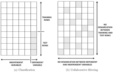
3.3 Data entries in a classification and collaborative filtering setting. . . 27
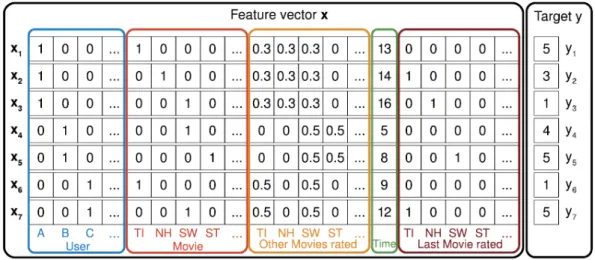
4.1 Example of movie input data for a factorisation machine. . . 40
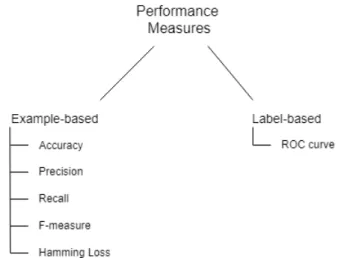
5.1 Performance measures for multi-label classification. . . 60
5.2 Confusion Matrix. . . 61
6.1 Frequency barplot of the MovieLens 100K ratings. . . 66
6.2 Frequency barplot of the LDOS-CoMoDa ratings. . . 67
6.3 Boxplots of the RMSE and the MAE obtained by different algorithms on sparsity level 99% and 98% on the MovieLens dataset. . . 71
6.4 The mean and the standard error of the RMSE and the MAE obtained by different algorithms on sparsity level 99% and 98% on the MovieLens dataset. The bars indicate the mean while the dots indicate the standard error. . . 72
6.5 Boxplots of the RMSE and the MAE for algorithms having either the lowest RMSE, MAE or run time on sparsity level 99% and 98% on the MovieLens dataset. . . 74
6.6 Boxplots of the RMSE and the MAE obtained by different algorithms on sparsity level 99%, 98% and 95% on the LDOS-CoMoDa dataset. . . 75
LIST OF FIGURES xi
6.7 The mean and the standard error of the RMSE and the MAE obtained by different algorithms on sparsity level 99%, 98% and 95% on the LDOS-CoMoDa dataset. The bars indicate the mean while the dots indicate the standard error. . . 75 6.8 Boxplots of the RMSE and MAE for algorithms having either the lowest RMSE, MAE or run
time on sparsity level 99%, 98% and 95% on the LDOS-CoMoDa dataset. . . 77 7.1 Prediction performance of the MLC algorithms on LDOS-CoMoDa and TripAdvisor datasets. 83 7.2 LDOS-CoMoDa: Boxplot of performance measures for the different baseline recommenders. . 85 7.3 TripAdvisor: Boxplot of performance measures for the different baseline recommenders. . . . 86 7.4 Prediction performance of baseline algorithms. Precision, recall, accuracy and F1 values are
read off the left axis, while Hamming loss is read off the right axis. . . 87 7.5 Prediction performance of all algorithms. Precision, recall, accuracy and F1 values are read
List of Tables
1.1 Application Domains of Recommender Systems. . . 1
1.2 A book database. . . 4
1.3 Users’ ratings of books. . . 5
4.1 An artificial movie dataset. . . 46
4.2 Observation from an artificial movie dataset. . . 46
4.3 Number of parameters in various factorisation machines models. . . 48
5.1 Multi-label dataset represented as a matrix. . . 54
6.1 Description of the two datasets: MovieLens and LDOS-CoMoDa. . . 65
6.2 Format of the MovieLens rating file. . . 66
6.3 Format of the LDOS-COMODA rating file. . . 66
6.4 Proportions of user ratings in the original MovieLens dataset. . . 69
6.5 Selecting users for different sparse matrices. . . 69
6.6 Algorithms used in experiments. . . 70
6.7 The mean and standard error of the RMSE and MAE obtained by different algorithms on sparsity level 99% and 98% on the MovieLens data. The average time (in seconds) it took the algorithms to run is given in the last column. . . 73
6.8 The mean and standard deviation of the RMSE and MAE obtained by different algorithms on sparsity level 99%, 98% and 95% on the LDOS-CoMoDa dataset. The average time (in seconds) it took the algorithms to run is given in the last column. . . 76
7.1 Description of the context-aware datasets: LDOS-CoMoDa and TripAdvisor. The values in brackets next to the context variables indicate the number of dimensions that each context has. 81 7.2 Hamming Loss values for each regression algorithm. . . 90
7.3 F-measure values for each regression algorithm. . . 90
7.4 Accuracy values for each regression algorithm. . . 91
LIST OF TABLES xiii
B.1 Algorithm parameters used for the models on the MovieLens dataset at sparsity level 99% and 98%. . . 120 B.2 Algorithm parameters used for the models on the LDOS-CoMoDa dataset at sparsity level
List of Abbreviations
AFM Attentional Factorisation Machine ALS Alternating Least Squares
BP-MLL Back-Propagation Multi-Label Learning
BR Binary Relevance
BR-kNN Binary Relevancek-nearest Neighbours
CARS Context-Aware Recommender System
CB Content-based
CC Classifier Chains
CF Collaborative Filtering
CTR Click Through Rate
CW Curds-and-Whey
FM Factorisation Machine
FFM Field-Aware Factorisation Machine FICYREG Filtered Canonical Y-variate Regression FwFM Field-Weighted Factorisation Machine
GP Global Popular
HOFM Higher-Order Factorisation Machine IDF Inverse Document Frequency IFS Information Filtering System IMDb Internet Movie Database
LIST OF TABLES xv
IP Item Popular
LFM Latent Factor Model
LP Label Powerset
MAE Mean Absolute Error MF Matrix Factorisation MLC Multi-Label Classification
ML-RBF Multi-Label Radial Basis Function ML-kNN Multi-labelk-nearest Neighbours
NMF Non-Negative Matrix Factorisation OLS Ordinary Least Squares
PCA Principal Component Analysis
PITF Pairwise Interaction Tensor Factorisation RAkEL Randomk-labelsets
RARS Remedial Actions Recommender System RMSE Root Mean Squared Error
RR Reduced Rank
RS Recommender System
SGD Stochastic Gradient Descent
SPTF Scalable Probabilistic Tensor Factorisation SVD Singular Value Decomposition
SVM Support Vector Machine
TF Term Frequency
TF-IDF Term Frequency Inverse Document Frequency
UP User Popular
Chapter 1
Introduction
Since its invention by Tim Berners-Lee in 1989 (Berners-Lee, 1989), the growth of the World Wide Web has facilitated the ease with which knowledge may nowadays be shared. However, the resulting abundance of information may quickly cause web users to experience information overload (Maket al., 2003). When presented with any form of information, humans tend to naturally filter out details that are irrelevant to them. Consider, for example, the decision to buy a magazine. We expect a person to buy a magazine that is particular to his/her interest, such as travel or cookery. Furthermore, within that magazine, an individual would only take note of articles that he/she finds appealing. An Information Filtering System (IFS) does this on a much larger scale. More specifically, the objective of an IFS is to narrow the amount of information shown to a user, based on their preferences, in an automatic way. A Recommender System (RS) is a particular type of information filtering system. It aims to reduce the volume of information presented to an individual, by suggesting items (for example books, movies, or websites) that correspond to their specific interests and requirements (Burke, 2002). According to the taxonomy of recommender systems described by Montaneret al.(2003), recommender systems may be organised into four general domains, depending on the type of content that they recommend. These domains, which by far the majority of recommender systems focus on, are entertainment, content, e-commerce and services. More recently, some research has been devoted to recommendations during data exploration, data visualisation, and work-flow design. These areas are explored by Drosou and Pitoura (2013), Ehsanet al.(2016) and Jannachet al.(2016), respectively. The items that may be recommended in the aforementioned domains are named in Table 1.1.
Table 1.1: Application Domains of Recommender Systems.
Entertainment Movies, music
Content Documents, web pages, newspapers
E-commerce Products to purchase, such as fashion, books, furniture Services Accommodation, beauty salons, travel services, restaurants Databases Data exploration, data visualisation, work-flow design
CHAPTER 1. INTRODUCTION 2
The simplest type of recommendations are given by non-personalised recommenders, which are not unique to an individual or user. Non-personalised recommenders suggest items that may be interesting to all users. Certain events may acquire a large amount of attention in a short period of time, causing them to appear in a ‘trending’ section, such as on the video streaming site YouTube. The most popular product might be recommended on an e-commerce website, while a magazine might list the top ten bestselling books of the month. Since non-personalised recommenders generally recommend the most sought-after items, they are very straightforward to implement.
On the other hand, personalised recommenders guide users to items that are most likely to meet their particular needs. Therefore, the recommendations provided by a personalised RS will differ greatly between users. In this study, we focus on personalised recommenders (as does most research in this field). Personalised recommenders are useful not only to the users of the system, but to the service provider (Ricci et al., 2011). E-commerce websites which make use of personalised recommendations have been shown to have a huge positive impact on sales revenue. These websites display items particular to users’ interests, and therefore user satisfaction is improved. As users are more likely to purchase products that appeal to their needs, the number of items sold by the provider is likely to increase. An example of such a recommender is Netflix, the well-known online movie and TV show streaming service. Netflix provides recommendations that are based on users’ past preferences, thereby allowing a user to easily select a new movie to watch. By providing reliable recommendations, Netflix was able to save approximately $1 billion dollars by preventing customer churning (Gomez-Uribe and Hunt, 2015). The online store Amazon also experienced an improved turnover from implementing a recommender system. It was estimated that 35% of the sales on Amazon emanate from accurate recommendations (MacKenzieet al., 2013). Thus, we can see that personalised recommenders have an added advantage over non-personalised recommender systems. In our study, we focus on two types of personalised recommendations. In the first type of recommendation, we consider the typical problem of recommending a new item to a user that they are most likely to enjoy. The second type of recommendation that we consider is suggesting the best context in which an item should be consumed by the user.
In the remainder of this chapter, we discuss the general ideas underlying recommender systems. The notation which is commonly used in an RS context, and based largely on the notation utilised by Lops et al.(2011) and Desrosiers and Karypis (2011), is also established. We introduce the notation, along with concepts and terminology that are fundamental to the study of recommender systems in Section 1.1. The format in which data may be stored in an RS database is discussed in Section 1.2, while the most common types of recommender systems are introduced in Section 1.3. In Section 1.4 we describe key factors that need to be considered when designing an RS. Following this, common metrics used for the evaluation of recommenders are discussed in Section 1.5. The purpose of our study is given in Section 1.6 and we close this chapter with an overview of the thesis, given in Section 1.7.
CHAPTER 1. INTRODUCTION 3
1.1
Concepts, Terminology and Notation
The terms users and items are continually used when discussing recommender systems. Objects to be recommended by the system, such as movies, clothing, or books, are generally referred to as items. Individuals who make use of the system in order to find items to their liking, are calledusers.
LetU ={u1, u2, . . . , un} andI={i1, i2, . . . , im} respectively denote the set ofnusers andmitems in a system. Let also the recorded ratings in the system be denoted by the setR, and the values that these ratings may assume be contained in the setS.
We assume that each user is allowed to rate a particular item only once, and let the rating given by a useru∈ U to an item i∈ I be denoted byrui. The subset of items rated by useruis denoted by Iu, and similarly, the subset of users that have rated itemiis given byUi. To denote the exclusion of a set
Iu from a setI, we use the notationI \ Iu. Also, note that we usually use the notation |X | to denote the number of elements in the setX. When we need to avoid confusion with the absolute value sign, we use the notationn(X)instead. Typically, when referring to a specific user under consideration, he/she
is called theactive user, represented byua.
Based on users’ feedback, an RS aims to determine which items a particular user is likely to enjoy. An RS may obtain feedback in an implicit or explicit manner. Alternatively, implicit and explicit feedback may be combined. Explicit feedback entails users directly evaluating objects, while implicit feedback is obtained in an indirect manner, for example by monitoring users’ activity on the system.
Explicit feedback is incredibly useful since it allows the system to learn exactly how the user perceives an object (Levinas, 2014). Although rating objects seems to be a simple task, it may happen that users interpret rating scales differently. For example, two users may in fact both like an item, but one may be more generous in their rating than the other. A further drawback of explicit ratings is that they are difficult to acquire. Users may find it tedious and inconvenient to rate items after consuming them, or they might simply forget. Thus no rating is obtained for that user regarding the item.
In contrast to explicit feedback, implicit feedback does not require the user to actively state their prefer-ences. Instead, the system attaches relevance scores to users’ actions in order to decide if a specific user values a particular acquired object (Lopset al., 2011). Implicit feedback tends to be less biased. For example, there is no need for the user to rate an item highly simply because it seems to be popular at the moment. There are, however, drawbacks to this form of feedback. The system will assess a user’s actions, such as browsing time or purchase history, and base recommendations on these. Whereas an item purchased by a user should imply that the user likes the item, he/she may have purchased it for someone else, or the account could be shared among individuals.
CHAPTER 1. INTRODUCTION 4
(Schaferet al., 2007). These include binary, ordinal, numerical, and unary rating scales. Since some scales are more suited to certain contexts, the type of rating scale utilised typically depends on the RS domain. When a binary rating scale is implemented, a user is simply asked to decide whether an item is good or bad. An example is the ‘thumbs up’ and ‘thumbs down’ feature on YouTube. Surveys or questionnaires generally make use of ordinal scales, where the user selects the level to which they agree with a statement. For example, a user will select from the list {strongly agree, agree, neutral, disagree, strongly disagree}. One of the most well-known rating scales is the numerical scale, where a user expresses his/her interest by a1-to-Nrating, where1indicates complete disinterest or dislike, andNindicates that the user thoroughly
enjoyed the item. Finally, unary ratings are typically associated with the situation where there is only an option for ‘liking’ the item, and not for ‘disliking’ it. An example of unary ratings may be found on the social media platform Facebook, where users can ‘like’ a post, but not ‘dislike’ it (Aggarwal, 2016). Note that unary ratings may also be collected as part of a user’s implicit feedback, where the time spent viewing an item, or purchasing it, would convey to the system that a user is interested in the item.
1.2
Data Representation
A database is used to store information concerning items that may be recommended to a user. The database can take on either a structured or an unstructured format. In the case of a structured database, a set of features or attributes are used to describe the items. The features remain the same for all items, and each feature can assume a known set of values. For example, consider Table 1.2, which depicts the first five entries in a very simple database concerning books. Each row represents a book, while the columns represent the features. A unique ID is assigned to each book in order to ensure that books can be distinguished from each other, should there be more than one book with the same title.
Table 1.2: A book database.
Item ID Title Author Year Genre
i01 Jane Eyre Charlotte Bronte 1847 Social Romance
i02 Pride and Prejudice Jane Austen 1813 Romance
i03 Dune Frank Herbert 1965 Science fiction
i04 Ender’s Game Orson Scott Card 1985 Military science fiction
i05 The Hobbit J. R. R. Tolkien 1937 Fantasy
On the other hand, unstructured data do not contain observations with clearly defined features. Therefore, unstructured data cannot be arranged in row and column format as seen in Table 1.2. An example of an unstructured database would be an audio or video file, or a collection of product reviews.
Figure 1.1 is an excerpt of a product review taken from Amazon. Each review is different in terms of style, length and language, and therefore has no structure. Typically, a mixture of structured and unstructured data are used in recommender systems, thereby causing RS databases to be semi-structured.
CHAPTER 1. INTRODUCTION 5
Figure 1.1: An example of a product review on Amazon Source: Amazon [Online].
An RS database will also store the ratings that a user has given items. Consider again the book database in Table 1.2. The ratings that usersu01andu03have given to the different books are shown in Table 1.3.
From Table 1.2 and Table 1.3 we can deduce thatu01is likely to enjoy romance books, while u03 would
rather read science fiction.
Table 1.3: Users’ ratings of books.
User ID Item ID Rating
u01 i01 4
u01 i02 3
u03 i02 1
u03 i03 5
u03 i04 4
1.3
Types of Recommender Systems
Most frequently in the literature, personalised recommender systems are categorised into three main classes,viz. content-based, collaborative filtering, and hybrid approaches. There are, however, also more extensive taxonomies, as given for example in Burke (2002). Thereby, recommender systems may be partitioned into content-based, collaborative filtering, knowledge-based, demographic and hybrid systems. When deciding between these recommenders, there are a number of factors that should be taken into consideration. The type of information available, the domain in which the recommendations are to be made, as well as the algorithms to be used, can play a role in selecting the type of recommender system to implement (Montaneret al., 2003).
We focus in this section on the way in which the type of data used by an RS determines the way in which it may be categorised. In the RS context, it is possible that the only available data is the ratings given by users to items. In certain domains, external knowledge, such as attribute information associated with sets of users and items, may also be available. Keeping the above data scenarios in mind, we provide brief descriptions of the five different recommender strategies identified in Burke (2002).
CHAPTER 1. INTRODUCTION 6
In Content-based (CB) systems, the item features and the ratings that a user gave to items are used to recommend new items. Content-based recommendation is based on the idea that the user is likely to enjoy new items that have similar features to the ones that they have enjoyed in the past. Since only the items that an active user has rated in the past are considered when making recommendations, content-based recommendation is user-specific. By not exploiting interactions between different users in the system, clearly CB methods are severely limited. A news recommender system, called NewsWeeder, is an example of one of the earliest content-based recommenders (Lang, 1995).
Collaborative Filtering (CF) systems find users that have rated items similarly to the active user, and make recommendations based on these similar users. In other words, recommendations are based on the idea that the active user should enjoy items that users with a similar taste to them have enjoyed. The first implementation of this type of recommender is attributed to Goldberget al.(1992). The two types of CF algorithms are memory- and model-based. The former is further divided into user- and item-based CF. The latter is based on using typical regression or classification models to make a recommendation. The main drawback of a CF system is that an item needs to have been rated before it can be recommended, or a user has to have rated an item before they can receive recommendations. In other words, a sufficient amount of information is needed regarding the items and/or users before recommendations can be made. Scenarios where this is not the case, i.e. if there is no information available regarding certain users’ preferences, or on certain item ratings, are referred to as occurrences of thecold-start problem. If many item ratings are missing, the data to be used to in the RS can become very sparse. Several model-based algorithms have been proposed in an attempt to alleviate the data sparsity problem, such as latent factor models, which are based on Singular Value Decomposition (SVD).
A knowledge-based system aims to meet users’ requirements by using domain knowledge about the items, as well as information on user preferences. Knowledge-based systems are useful for recommending items that are seldom purchased, and therefore associated with either a limited number of ratings, or no ratings at all. An example of such a system is the online classified advertisement website, Gumtree1, where users input certain requirements they need from an item, and the recommender determines which items best match these needs.
In a demographic RS, rather than only relying on ratings or item information, the available demographic information of a user is used to make a recommendation. Users are grouped together according to the demographic information that they have provided, such as age, gender or location, and based on the group or niche into which a user falls, a recommendation is made. The drawback of this method is that demographic data is generally difficult to acquire due to privacy concerns, therefore the applications are often limited. In the paper by Wanget al.(2012), they consider the recommendation of tourist attractions using this approach on data from TripAdvisor. Different machine learning algorithms are considered to
CHAPTER 1. INTRODUCTION 7
group users according to their demographic information. A recommendation is made to the active user by identifying to which class they belong, and then suggesting an attraction based on the ratings of the users in the identified class.
When various forms of inputs are available, it is possible to use different types of recommender systems. Hybrid recommender systems, as the name suggests, are mixtures of the above mentioned techniques. They allow for the incorporation of the useful qualities of one system to be used in conjunction with an-other system that lacks these qualities. For example, content-based recommenders do not suffer from the new item problem as they rely on the content of items. Collaborative filtering systems, however, cannot recommend an item that has no ratings. Thus, by combining these two techniques, the performance of a RS is no longer impaired by not being able to suggest new items (Ricciet al., 2011).
1.4
Properties of Recommender Systems
One of the most desirable properties of an RS is that it provides accurate suggestions to users. The accuracy is typically measured using one of several evaluation metrics, to be discussed in Section 1.5. However, there are a number of other factors that should also be considered when designing an RS. Common properties to be considered include scalability, robustness, diversity, novelty and serendipity. While we provide a brief description of each of these factors, a more extensive examination may be found in Aggarwal (2016) and in Shani and Gunawardana (2011). Moreover, metrics used to evaluate recommender systems based on a number of these factors can be found in Kaminskas and Bridge (2016). • Scalability. As the number of users and items in an RS increases, the volume of data in the form of
explicit and implicit ratings also increases. This means that the size of a database for recommender systems continues to grow over time. An important consideration therefore is whether an RS is able to provide good recommendations in an efficient and effective manner, even on very large datasets. The scalability of an RS is typically assessed in terms of training time, prediction time and memory requirements.
• Robustness. A recommender system is said to be ‘under attack’ when false or fake ratings are
purposefully entered into the system. This is generally done in order to skew the popularity of an item. For example, a restaurant owner might create false profiles to leave positive reviews for their restaurant, while leaving negative ones for the surrounding restaurants. An RS is said to be robust when its recommendations remain stable and unaffected by such fake ratings.
• Diversity. Consider the top five recommendations provided by a book recommender. If the
recommender suggests books written by only one author, its recommendations are very similar. If the active user does not like the first recommendation, it is very likely that he/she will not enjoy
CHAPTER 1. INTRODUCTION 8
any of the remaining books. Hence, in such a case, no useful recommendations were provided. It therefore seems sensible to require an RS to provide recommendations that are diverse in nature. Diversity can be measured using the similarity between items.
• Novelty. When an RS recommends items that the active user was previously unaware of, the
recommendation is said to be novel. An easy way to ensure novelty is to remove items that the user has rated from the list of recommended items. A user-study can be conducted in order to determine the novelty of an RS. The users will be asked to explicitly state whether or not they have seen the items before.
• Serendipity. A recommendation which is new and unexpected, but enjoyed by a user, may be
regarded as aserendipitous recommendation. Serendipitous recommendations are novel, however novel recommendations are not necessarily serendipitous. This is because the only requirement of a novel recommendation is that the user should previously have been unaware of the item. Geet al. (2010) and Kotkovet al.(2016) discuss methods to evaluate the serendipity of an RS.
1.5
Evaluation of Recommender Systems
In this section we consider common metrics used for the evaluation of recommender systems. This discussion is based largely on Desrosiers and Karypis (2011).
One may view the item recommendation task to be either a prediction or ranking task (Han and Karypis, 2005). In a prediction setup, the aim is to obtain the single (best) item deemed most likely to be of interest to the active user. This means that for userua, a single, unseen itemi∈ I \ Iua is proposed. In
other words, we aim to either predict a numerical rating for an unseen item, or to classify an unseen item according to, for example, a binary or ordinal scale. This formulation of the recommendation problem clearly fits into a regression or a (multi-class) classification framework.
In order to evaluate a best item recommender, before the recommender is built, the set of ratingsRare divided into a training setRtrain and a test setRtest. Let f be a function such thatf : U × I → S. UsingRtrain, we then learn the modelfˆ, and for each item i ∈ I \ Iua, the rating that userua would
give to the item is predicted via the functionfˆ(u, i). The itemi∗with the highest rating is shown to the user, where
i∗ = arg max ˆf(ua, j) j∈I\Iua
. (1.1)
When ratings are predicted, the accuracy measures commonly used to evaluate the system are the Mean Absolute Error (MAE) or the Root Mean Squared Error (RMSE). These are given by Equations 1.2
CHAPTER 1. INTRODUCTION 9 and 1.3, respectively. MAE( ˆf) = 1 n(Rtest) X rui∈Rtest |fˆ(u, i)−rui|,and (1.2) RMSE( ˆf) = s 1 n(Rtest) X rui∈Rtest ( ˆf(u, i)−rui)2. (1.3) When explicit ratings are unavailable, and only the purchase history of the active user is available, for example, we have a ranking setup. This is commonly used in content-based recommendation, where the system recommends items that are similar to the items previously purchased by the user. Here, a list
L(ua) of N items that a user ua would most likely enjoy are displayed. The value ofN is typically a small value decided before recommendations are made.
For evaluation purposes, before the recommender is built, the itemsI are split into a training and test set, denoted byItrain andItest, respectively. Additionally, a test user is selected and the subset of test items that the user has purchased is denoted byT(u)⊂ Iu∩ Itest. The two most common measures to assess the performance of an RS that recommends a list of items are precision (Equation 1.4) and recall (Equation 1.5). Whereas precision is the proportion of items predicted to be relevant that are in fact relevant, recall is the proportion of actual relevant items that have been suggested.
Precision(L) = 1 |U | X u∈U 1 |L(u)||L(u)∩T(u)|,and (1.4) Recall(L) = 1 |U | X u∈U 1 |T(u)||L(u)∩T(u)|. (1.5) Using the method of displaying a list ofN recommendations means that the user is inconvenienced by
the fact that all items are regarded as being equally applicable (Desrosiers and Karypis, 2011). In other words, no specific item is presented as being more likely to be enjoyed by the user, and so the user would still have to determine this for himself from the given listL.
It is also possible that the goal of the recommender is not to suggest items to users, but rather, for example, tags associated with items or even the context in which the item should be used. The formulation clearly fits into a mulit-label classification framework. The metrics used for the evaluation of the recommender may also be precision and recall.
1.6
Purpose of the Study
1.6.1
Motivation
With the exponential growth of information being readily available to individuals, recommender systems are proving to be crucial in reducing information overload. A number of studies have been conducted
CHAPTER 1. INTRODUCTION 10
comparing the performance of recommender algorithms. A comparative study of algorithms was con-ducted by Stomberg (2014), however only user-based, item-based and SVD algorithms were considered. Furthermore, the effect of data sparsity on the algorithms was not considered. Cremonesiet al.(2010) present a similar comparison of non-personalised algorithms, neighbourhood methods and latent factor models on two movie datasets. The methods are evaluated based on top-N recommendation, therefore
the metrics used are precision and recall. As in Stomberg (2014), sparsity is not considered.
As the field of recommender systems is ever-expanding, there is scope for an extended comparison of recommender algorithms, beyond that of the traditional approaches considered in the above mentioned papers. In order to understand the state-of-the-art approaches, a thorough study of the traditional approaches is necessary and is therefore also included in this study. Furthermore, the task of mendation typically focuses on the recommendation of an item to a user, and does not consider recom-mending appropriate contexts in which to consume the item. This leads to a further avenue of research, namely recommendation via the use of label classification methods. Some recently proposed multi-variate regression approaches to MLC assist with the interpretability of MLC output. As explainable recommender systems is an important topic of interest in RS research, we believe the use of MLC in recommender systems to be a promising research direction.
1.6.2
Objectives
The aim of this thesis is to provide an overview of both the traditional and more recent, state-of-the-art algorithms used for recommender systems. We aim to:
• Demonstrate the construction and properties of different types of recommender algorithms. • Empirically investigate the effects of data sparsity on their performance.
• Test the validity of the use of various MLC approaches for the recommendation problem.
1.7
Thesis Overview
The remainder of the thesis may conceptually be partitioned into two main sections. Chapters 2 to 5 provide an overview of the various recommendation techniques, while in Chapters 6 and 7 we report on our empirical work.
In the first part of the thesis, we start with an overview of content-based recommender systems in Chapter 2. The architecture and data pre-processing steps for this class of recommender systems are described, and augmented with a discussion of the advantages and disadvantages of content-based recom-menders. In Chapter 3 we consider the most popular method of recommendation, namely collaborative filtering. The two CF approaches and their main drawbacks are discussed. This leads us to an overview
CHAPTER 1. INTRODUCTION 11
of more advanced CF methods in Chapter 4, where we we consider extensions to model-based CF, known as Latent Factor Models (LFMs). The latter class of models aim to address the data sparsity problem. For an overview of an entirely different perspective on the recommendation problem, in Chapter 5 we approach the recommender problem from a multi-label classification point of view. Both established and more recently proposed (regression) approaches to MLC are described. Performance measures deemed relevant in an MLC context, are also given.
The second part of the thesis is devoted to a discussion of the two empirical studies undertaken during the study. The first empirical study, with the aim of evaluating the impact of data sparsity on various CF and LFM algorithms, is described in Chapter 6. The second empirical study was carried out in order to investigate the use of MLC algorithms in the context of recommender systems. The MLC experiments and results are discussed in Chapter 7. We conclude the thesis in Chapter 8, with a summary, and with a few suggestions regarding avenues for further research.
Chapter 2
Content-based Recommenders
2.1
Introduction
The focus of this chapter is on one of the two main approaches to personalised recommenders, namely content-based recommendation. Based on items that a given user has previously liked or rated, a Content-based (CB) recommender systems suggests similar items to a user. The idea underlying CB recommender systems is that a user should enjoy new items that have features in common with items that they previously enjoyed. For example, a movie recommender might suggest new movies that have the same genre as the movies that the user enjoyed in the past. In order to make these recommendations, the content of the active user’s rated items are examined, thereby creating a unique user profile (Balabanović and Shoham, 1997).
Therefore, in content-based recommendation, descriptive profiles are needed for the users. These profiles often rely on external information regarding the items. For example, in the case of a movie recommender, commonly used item information include movie genre and actors, or tags used to describe the movie. In this way, Magnini and Strapparava (2001) developed a movie recommender by analysing movie synopses available from Internet Movie Database (IMDb). Another successful implementation of content-based fil-tering is a book recommender called Learning Intelligent Book Recommending Agent, or LIBRA (Mooney and Roy, 2000). Here, product descriptions, available from the online store Amazon, were analysed and a bag-of-words naive Bayesian text classifier was used to learn a user profile.
The remainder of this chapter is structured as follows. The architecture of a CB recommender system is discussed in Section 2.2, followed by an overview of a regularly employed technique which is used by CB recommender systems in order to represent items in a meaningful way. This overview may be found in Section 2.3. As a simple illustration, we discuss how linear regression can be used to learn a user profile in Section 2.4. A discussion of the advantages and common problems that may be expected when using a CB recommender system may be found in Sections 2.5 and 2.6, respectively. We conclude the chapter
CHAPTER 2. CONTENT-BASED RECOMMENDERS 13
with a summary in Section 2.7.
2.2
The Architecture of Content-based Recommenders
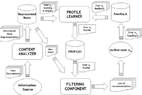
The main components of a CB recommender are the Content Analyser, the Profile Learner and the Filtering Component. Each component is responsible for a different step in the recommendation process. In short, the Content Analyser receives the items and converts them into a usable format. The Profile Learner aims to use feedback in order to discover the preferences of a user, whereafter the Filtering Component uses the learned profile to recommend new items to an active user.
Figure 2.1: The input of the Content Analyser. Source: Desrosiers and Karypis (2011).
The Content Analyser is responsible for the first step in the recommendation process. As seen in Fig-ure 2.1, this component receives items from some information source. Examples of information sources are web pages, journals, and social media platforms. An information source contains descriptions of the items, which the Content Analyser may then convert into a usable format.
In the case of structured data, the CB recommender is said to be feature-based, while in the case of un-structured data, the CB recommender is described as text categorisation-based (Mooney and Roy, 2000). Difficulties arise when incorporating unstructured data (such as unrestricted text) into a recommender system. Unrestricted text can include product descriptions, item tags, movie synopses or news articles, to name a few. So-called Vector Space Models (VSMs) were developed for the purpose of semantic text processing, and may successfully be used in order to transform unstructured text into a structured data matrix. The use of VSMs in text analysis is a very specialised field. Hence, in Section 2.3 we only briefly discuss the use of VSMs in order to shed some light on the way in which text can be used as input in a CB recommender.
After converting unstructured data to a structured item representation, as shown in Figure 2.2, the resulting data matrix may be passed on to the Profile Learner component. Consider an active userua. Using itemsIua rated byua, an initial user profile may be constructed. In more detail, for a given user
CHAPTER 2. CONTENT-BASED RECOMMENDERS 14
Figure 2.2: The output of the Content Analyser. Source: Desrosiers and Karypis (2011).
Figure 2.3: The input of the Profile Learner. Source: Desrosiers and Karypis (2011).
ua we have available a training set consisting of ratings on K items. That is, we have the item-rating pairsTak={(iak, rak),k= 1,2, . . . , K}, where Kis the total number of items rated byua.
A user’s preference may be inferred based upon items he/she has previously rated. The Profile Learner receives represented items that have been rated by a given user (Figure 2.3), and applies supervised learning techniques to build a predictive profile (or model) for the user. These techniques include, but are not limited to, linear classifiers, Naive Bayes classifiers, decision trees,k-nearest neighbour algorithms,
and relevance feedback. In Section 2.4, we consider how the user profile is learned using a linear classifier. Once complete, the learned profile is stored in the Profiles Archive, as depicted in Figure 2.4.
The user profiles, together with items that have not yet been rated by the active userua, are finally passed to the Filtering Component (Figure 2.5). This component is used to suggest items to the user that he/she may find interesting. This is done by comparing the learned profile to features of the new represented items, and by determining which of the new items are the most similar to the learned profile. A list of items is suggested to the user, ordered according to their preference, as deduced by the Filtering Component.
CHAPTER 2. CONTENT-BASED RECOMMENDERS 15
Figure 2.4: The output of the Profile Learner. Source: Desrosiers and Karypis (2011).
Figure 2.5: The input of the Filtering Component. Source: Desrosiers and Karypis (2011).
Of course the taste of a user may change over time. Therefore, in order to ensure that recommendations are as accurate as possible, the user profile should continually be updated. For this purpose, feedback may (either implicitly or explicitly) be acquired and used by the Profile Learner in order to update the profiles.
Finally in this section, the individual components of a content-based recommender system are combined in Figure 2.6, thereby conveying its general architecture.
CHAPTER 2. CONTENT-BASED RECOMMENDERS 16
Figure 2.6: Architecture of a Content-based Recommender System. Source: Desrosiers and Karypis (2011).
2.3
Item Representation in Content-based Recommenders
Given a set of items, together with a user, a content-based recommender system needs to find similar (or other relevant) items for the user. As mentioned, it is often the case with content-based recommenders that items are not represented by a defined set of features, but rather by textual descriptions. Therefore, the Content Analyser needs to convert the textual features into a usable format. In this section, we describe how this process may be carried out.
A traditional feature extraction technique used in information retrieval to achieve a structured repres-entation of textual data is a vector space model. A VSM is an algebraic model that is used to spatially represent a set of items, and can assist an RS in determining the similarity between items. This is achieved in two steps,viz. a pre-processing step, followed by the calculation of term weights.
Phrases, keywords or single words used to describe an item are referred to as ‘terms’. During the preliminary processing of items, all punctuation, special characters and stop-words in the item descriptions are removed. A so-called bag-of-words representation is then used to represent the items, and each unique word used to describe the items is used as a feature. In other words, each item is subsequently represented as a vector of words (terms). For each item, the presence or absence of a particular word can then be indicated either by the number of times that it appears in the item description, or by a Boolean value. Next, the term vectors are converted into a usable numerical format, known as a vector of term weights. These term weights indicate how closely each term is related to an item. The frequency distribution of terms within an item description, as well as within the entire collection of terms used to describe all the items, plays an import role in determining how meaningful a term is.
CHAPTER 2. CONTENT-BASED RECOMMENDERS 17
A commonly used method for calculating term weights is Term Frequency Inverse Document Frequency (TF-IDF) (Turney and Pantel, 2010). As explained by Lops et al. (2011), TF-IDF is based on the characteristics of text documents. A frequently occurring word in an item description (Term Frequency (TF)) is more closely related to the item if it occurs infrequently throughout all the item descriptions (Inverse Document Frequency (IDF)). Before expanding on how term weights are calculated in TF-IDF, we first import some notation, following the notation introduced by Lopset al.(2011).
Let the set of item descriptions be denoted by I={i1,i2, . . . ,im}, and let the entire set of unique terms found in I after pre-processing the item descriptions be given by T ={t1, t2, . . . , t|T|}. The n -dimensional item vectors are denoted by ij = {w1j, w2j, . . . , wnj}, where wkj indicates the weight for termtk, k= 1,2, . . . ,|T|, in itemij, j = 1,2, . . . , m. Additionally, let fkj be the number of times that termtk appears in the description of itemij. Note thatfkj is referred to as theraw count of termtk. The term frequency of an item may take on a number of forms. The simplest form is to directly use the raw count as the term frequency. The standard term frequency of itemij is calculated by dividing the raw countfkjby the number of terms in the item description, as is given in Equation 2.1.
TF(tk,ij) =
fkj
P
z∈ijfzj
. (2.1)
However, using Equation 2.1 alone allows for the possibility of items with shorter descriptions being ig-nored in favour of items with longer ones. This is because longer descriptions will contain a larger number of words, potentially allowing a particular word to have a higher count, regardless of its importance in the item description. Subsequently, we may want to rather make use of the so-called augmented frequency, given by Equation 2.2.
TF(tk,ij) = 0.5 + 0.5·
fkj
maxzfzj
. (2.2)
Intuitively, a term that occurs repeatedly throughout all item descriptions is uninformative. Therefore we want small weights to be associated with frequently occurring terms, and large weights to be associated with rare terms. In order to achieve this, we scale the TF using the IDF. Letnk denote the number of item descriptions in which the termtk appears at least once. Thus it follows that
IDF(tk) =
N nk
, (2.3)
where N is the total number of item descriptions. Scaling the TF by the factor in Equation 2.3 is,
however, quite severe. In order to dampen the effect of the IDF terms, we instead take the logarithm of the IDF term. Since the logarithmic function is a monotonically increasing function, we have that
log(nN
k) is non-negative whenever
N
nk is non-negative. To rephrase,
N
nk ≥ 1 implies that log(
N nk) ≥ 0.
Therefore, the TF-IDF function is given by
TF-IDF(tk,ij) = TF(tk,ij)log
N
nk
CHAPTER 2. CONTENT-BASED RECOMMENDERS 18
As a term occurs more frequently in the set of item descriptions (i.e. asnk increases), nN
k will tend to
one. This will in turn cause the IDF (and thus also the TF-IDF) to approach zero.
When using Equation 2.2 to compute term frequency, it is possible that the frequencyfkj of termtk in itemij is such thatfkj= maxzfzj. In this case,
TF-IDF(tk,ij) = log(
N nk
)
= IDF(tk). (2.5)
Equation 2.4 is often used to directly obtain the term weights. However, it is not uncommon to go one step further and normalise this equation. Normalisation ensures thatwij ∈[0,1]for all i = 1,2, . . . , n, andj = 1,2, . . . , N. Thus the final weight wkj for term tk in itemij is calculated using Equation 2.6, where|T|is the total number of words in set of item descriptions.
wkj = TF-IDF (tk,ij) q P|T| s=1TF-IDF(ts,ij)2 . (2.6)
A large value for wkj indicates that the wordtk is a particularly important distinguishing word in the description of itemij. That is, the wordtkoccurs frequently inij, but not throughout the entire collection of item descriptions. Small values imply that the wordtk appears frequently throughout the collection of item descriptions, and is therefore not a distinguishing word in the item description.
2.4
Learning A Profile
Recall that in a CB recommender system, each user profile is learned in isolation. That is, the learning process does not exploit similarities between users to assist in the recommendation process. As mentioned in Section 2.2, various supervised machine learning algorithms can be employed in order to construct a user profile, based on the contents of items rated by the user. When items are rated by users using a numeric scale, we view the recommendation process as a regression task. A user’s interests are modelled by a function learned by a machine learning algorithm. Once learned, the model (or user profile) is used to predict the user’s ratings of unseen items. Items are sorted according to their predicted ratings, and the items with the highest predicted ratings are recommended to the user. In this section, for a simple explanation, we focus our attention on linear regression as a means of learning a user profile.
In Section 2.3, we saw how item descriptions may be represented as vectors of word frequencies. The underlying assumption of using linear regression to predict ratings is that the ratings can be modelled as a function of the word frequency. Suppose we have a set of itemsI, as well was the entire set of terms
T found in I after pre-processing the item descriptions. Let Iu be ann× |T| matrix representing the
CHAPTER 2. CONTENT-BASED RECOMMENDERS 19
n-dimensional vector y. The linear model relating the word frequency to the user ratings is given by
y ≈ IuwT, (2.7)
where w is a |T|-dimensional row vector representing the coefficient (weight) of each word, and needs to be estimated. The n-dimensional vector of prediction errors for the model can be calculated using
Equation 2.8.
P E = IuwT −y. (2.8)
The linear model achieves maximum predictive performance when Equation 2.8 is minimised or, equival-ently, when the squared norm of the prediction errors are minimised. Therefore, we need to findw that
minimises
OF = ||IuwT −y||2+λ||w||2, (2.9) where λ >0 is regularisation parameter. The regularisation parameter λensures that the model does
not overfit to the training data, and the optimal value ofλcan be determined via cross-validation. The
weight vectorwis obtained by taking the gradient of Equation 2.9 with respect towand setting it equal
to zero. LetIbe a|T| × |T|identity matrix, then we have that
IuT(IuwˆT−y) +λwˆT = 0
=⇒ (ITuIu+λI) ˆwT = ITuy (2.10)
=⇒ wˆT = (ITuIu+λI)−1ITuy. (2.11) Since (ITuIu+λI) is a positive definite matrix, it is invertible. Therefore, Equation 2.11 follows from Equation 2.10.
LetXube anm× |T|matrix representing themtest items for useru. Furthermore, letwˆube estimated weight vector for useru. The ratings of these items can be predicted via Equation 2.12. The user model
can then be evaluated using, for example, the RMSE.
ˆ
y = XuwˆTu. (2.12)
Since a model is needed for each user in content-based recommendation, this process will be repeated for each user in the system.
2.5
Advantages of Content-based Recommenders
We have seen that content-based recommenders rely on the content of items rated by a user in order to learn a profile for that user. Each item is described by the same set of features, and recommendations
CHAPTER 2. CONTENT-BASED RECOMMENDERS 20
are made based on the similarity between items. This is advantageous in the sense that the RS can recommend items that have not been rated by any user before.
The user profile is based on items rated by the user, therefore the user knows exactly why an item is recommended to them. Thus, CB systems are transparent in their recommendations and users are more likely to trust the recommendations given to them. Another advantage of using only the active user’s ratings when creating a profile is user independence, meaning that the system does not need to rely on information from other users. In other words, even in the case of an item that has never been rated before, if that item’s features match those in the user profile, it may be recommended to the active user.
2.6
Limitations of Content-based Recommenders
One of the most common issues of recommender systems is the so-callednew user orcold-start problem (Burke, 2002). In order for the learned profile to accurately represent the user’s preferences, a sufficient number of items need to have been rated by the user. A new user will not have any rated items, and is therefore often prompted by the RS to give initial ratings to a set of initial items. However, due to the lack of training data, initial suggestions by the RS may not be applicable to the user.
Since the features of items are used in learning techniques employed by CB recommenders, the quality of the features is essential (Burkeet al., 2011). A learned profile will only be representative of the user if the items are described by detailed, key attributes. However, it is often difficult to acquire attributes for items. Furthermore, since a user profile has to be learned for each user in a CB system, content-based recommenders do not scale well with the number of users. Finally, a CB recommender can be subject to over-specialisation. This means that items are only recommended if they are very similar to ones already rated by a user (Iaquinta et al., 2008). Therefore, content-based recommenders tend to only present a narrow selection of recommendations to the user, and generally do not perform well in terms of the novelty and diversity of recommended items.
2.7
Summary
In this chapter, we discussed the way in which content-based recommenders aim to identify items with equivalent features to the items that a user has previously enjoyed. The architecture of a CB system, and the steps taken to make recommendations, were described. These steps include embedding unstructured features into a vector space, creating a user profile and finding items that are similar to a user profile. In terms of the advantages and limitations of CB recommender systems, it was noted that while these systems are transparent in terms of their recommendations and do not suffer from the new item problem, they generally do not supply novel or diverse recommendations.
Chapter 3
Collaborative Filtering Recommender Systems
3.1
Introduction
Unlike a content-based recommender system, a collaborative filtering recommender system does not make use of the content of items to make suggestions to a user. Instead, CF systems take advantage of a given user’s available rating history, together with the history of other users in the system, to determine the relevance of an item to an active user. CF recommender systems are based on the assumption that if two users have purchased or rated the same item, they are likely to share similar interests (Jannachet al., 2010). In other words, CF systems use the ‘wisdom of crowds’, orcollaboration among users to make predictions for an active user.
The idea of CF was presented by Goldberg et al. (1992), the authors of the first commercial recom-mender system called Tapestry. In this system, documents are recommended to users from a collection of electronic documents. The documents are sourced from email or news wire stories, for example. Users annotate the documents, which then allow the documents to be filtered according to preferences.
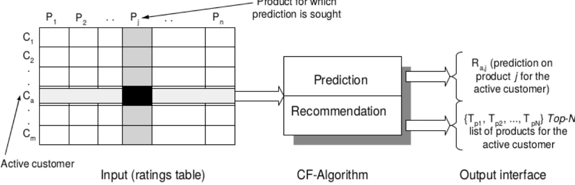
Figure 3.1: Collaborative Filtering Process. Source: Sarwar et al.(2002).
A high-level overview of the way in which a collaborative filtering system can make recommendations
CHAPTER 3. COLLABORATIVE FILTERING RECOMMENDER SYSTEMS 22
is depicted in Figure 3.1. The input to a CF system is a data matrix consisting of ratings allocated by the users to items which they have bought or viewed. These inputs in a so-called ratings matrixR, are
illustrated in the left part of Figure 3.1. Note that the rows{Ci, i = 1,2, . . . , m} represent users (or customers), and the columns {Pj, j= 1,2, . . . , n} represent items (or products in this application). The black square indicates that we are attempting to predict the ratingPj that user Ca would give to the itemj. An algorithm can be applied to the data to acquire this prediction, and outputs a recommendation
(or a list of recommendations) to the user. In other words, given a ratings matrix R, a collaborative
filtering system aims to estimate the two-dimensional rating functionhR given by
hR:U × I → S, (3.1)
whereU is the set of users, whereI is the set of items, and whereS is the set of possible values for the ratings.
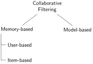
In this chapter, we explore the two approaches that CF recommender systems can apply to make pre-dictions, namely the memory-based (or neighbourhood-based) approach and the model-based approach (see Figure 3.2). In the former approach, the objective is to directly predict the relevance of an item to a user based on stored ratings. Since no assumptions regarding the functional form ofhR are made, the memory-based approach is a non-parametric approach. The two methods that can be used to do this (called user-based and item-based recommendation) form the focus of Section 3.2. On the other hand, in a model-based approach, we make an assumption regarding the functional form ofhR. Therefore, a model that is able to accurately predict missing item ratings needs to be learned. This approach is introduced in Section 3.3, and we continue the discussion in more detail in Chapter 4. Memory-based and model-based CF are compared in Section 3.4, followed by a comparison of content-based and collaborative filtering in Section 3.5. We summarise the chapter in Section 3.6.
CHAPTER 3. COLLABORATIVE FILTERING RECOMMENDER SYSTEMS 23
3.2
Memory-based Collaborative Filtering
Similarities between items or users play a pertinent role in memory-based CF recommender systems. In the memory-based approach, similar items (or users) are identified. The rating functionhR, given in Equation 3.1, is typically estimated using thek-nearest neighbour algorithm. Therefore the memory-based
approach is often referred to as a neighbourhood-based approach and, as the name suggests, similarities are calculated in-memory (Levinas, 2014).
Su and Khoshgoftaar (2009) separates the memory-based CF algorithm into three steps. The similarity between users (or items) are first calculated. Using these similarities, the ratings of new items are then predicted for an active user. This is followed by producing the recommended items that the user is most likely to enjoy. Depending on whether similarities between users or items are obtained, one may distinguish between user-based or item-based collaborative filtering. Stated very simply, the explanations associated with a recommendation from each method are:
User-based: "Similar users to you also liked..." Item-based: "Users who liked this item also liked..."
In other words, the goal of the user-based filtering is to identify users with similar preferences to the active user and to base the rating prediction on the ratings provided by these users, while item-based filtering finds similar items to the target item and bases the rating prediction on these item ratings. A well-known example of a user-based CF system is the music recommender Ringo, which employs the user-based technique to make recommendations (Shardanand and Maes, 1995). More recently, the CF approach Effective Trust (Guoet al., 2015), extends the user-based method to allow users to specify other users that they trust. This extension resulted in improved recommendation performance over that of a user-based recommender system. An example of an item-based CF approach is the Slope One approach (Lemire and Maclachlan, 2005). This method considers the differences between the ratings of items for users when predicting a new item.
3.2.1
User-based Filtering
In user-based filtering, we assume that users can be clustered into groups based on their preferences (Deshpande and Karypis, 2004). Similarities of users are based on the items they have consumed, as well as on how they have responded to them. To recommend items to the active user, his or her nearest neighbours (that is, the group of users he or she is most similar to) are identified. Based on the ratings given to items by the active user’s neighbours, new items are suggested by predicting the rating the active user would give to these items.
CHAPTER 3. COLLABORATIVE FILTERING RECOMMENDER SYSTEMS 24
More formally, consider anm×nratings matrix R, wherein the rating rui is missing since item i has not yet been experienced by useru. Our aim is therefore accurate prediction of ratingrui. We start by identifying thek users most similar to useru, and denote this set of neighbours byNk(u). The value of
kcan either be pre-specified, or an optimal value can be determined by means of a grid-search. Next, we
make use of the ratings for itemi, given by the neighbours of user u, in order to estimate rui. That is, we base the prediction ofrui on the set of ratings{rui˜,˜u∈ Nk(u)}.
In order to obtain Nk(u) for each user, of course some similarity measure is needed. There are many options in this regard. Arguably, two of the most frequently used similarity measures are the cosine similarity or the Pearson correlation. Letsuv denote the similarity between useruand userv. Then, the
suv-value according to the Pearson correlation is given by
suv = P C(u, v) = P i∈Iuv(rui−r¯u)(rvi−¯rv) q P i∈Iuv(rui−¯ru) 2P i∈Iuv(rvi−¯rv) 2 . (3.2)
In Equation 3.2,Iuv indicates the items rated by both usersuandv. Also, the mean rating of useruis defined as ¯ ru = 1 |Iu| X k∈Iu ruk, u= 1,2, . . . , n, (3.3) where |Iu| denotes the number of items rated by user u. Since Pearson correlation takes into account the differences in mean and variance of the ratings given by the usersuandv, the effects of users having
different rating habits are reduced. By subtracting the mean ratings, and by dividing by the standard deviations, the potential of some users rating items more generously than other users, does not influence the similarities between users as much.
In a regression setting, once the similarities between useruand all other users have been obtained, the
predicted ratingˆruiis calculated quite simply as the average rating given to itemiby the users inNk(u). That is, ˆ rui = 1 |Nk i(u)| X v∈Nk i(u) rvi, (3.4) where Nk
i(u) ⊆ Nk(u) denotes the subset of neighbours of u who have rated item i. A variation of Equation 3.4 is a weighted rating which takes the similarity between useruand uservinto account. This
implies that a rating given to itemiby a user who is very similar touwill be weighted more heavily than
a rating given toiby a user with dissimilar interests to u(Schaferet al., 2007). The weighted rating is calculated as follows: ˆ rui = P v∈Nk i(u)rvisuv P v∈Nk i(u)|suv| . (3

![Figure 1.1: An example of a product review on Amazon Source: Amazon [Online].](https://thumb-us.123doks.com/thumbv2/123dok_us/743634.2594120/21.892.335.561.518.634/figure-example-product-review-amazon-source-amazon-online.webp)