Gaussian processes for state space models and change point detection

(1)

Gaussian Processes for

State Space Models and

Change Point Detection

Ryan Darby Turner

Department of Engineering

University of Cambridge

A thesis submitted for the degree of

Doctor of Philosophy

(2)

(3)

Acknowledgements

I would like to thank Carl Rasmussen for advice throughout my PhD; Steven Bottone for extensive proof reading; Marc Deisenroth for as-sisting me in acquiring his LA_{TEX skills. I acknowledge my examiners}

Zoubin Ghahramani (internal) and Amos Storkey (external). I would like to thank my co-authors in the publications leading up to my the-sis: Yunus Saat¸ci, Carl Rasmussen, and Marc Deisenroth. I also thank the other proof readers in my group: David Duvenaud, Alex Davies, Ferenc Huszár, Dan Roy, Peter Orbanz, and José Miguel Hernández Lobato. I would like to thank Rockwell Collins, formerly DataPath, Inc., which funded my studentship. I also acknowledge my college, Magdalene College, and my laboratory, the Computational and Bio-logical Learning (CBL) laboratory.

(4)

This thesis details several applications of Gaussian processes (GPs) for enhanced time series modeling. We first cover different approaches for using Gaussian processes in time series problems. These are extended to the state space approach to time series in two different problems. We also combine Gaussian processes and Bayesian online change point detection (BOCPD) to increase the generality of the Gaussian process time series methods. These methodologies are evaluated on predictive performance on six real world data sets, which include three environ-mental data sets, one financial, one biological, and one from industrial well drilling.

Gaussian processes are capable of generalizing standard linear time ries models. We cover two approaches: the Gaussian process time se-ries model (GPTS) and the autoregressive Gaussian process (ARGP). We cover a variety of methods that greatly reduce the computational and memory complexity of Gaussian process approaches, which are generally cubic in computational complexity.

Two different improvements to state space based approaches are cov-ered. First, Gaussian process inference and learning (GPIL) general-izes linear dynamical systems (LDS), for which the Kalman filter is based, to general nonlinear systems for nonparametric system iden-tification. Second, we address pathologies in the unscented Kalman filter (UKF). We use Gaussian process optimization (GPO) to learn UKF settings that minimize the potential for sigma point collapse. We show how to embed mentioned Gaussian process approaches to time series into a change point framework. Old data, from an old regime, that hinders predictive performance is automatically and el-egantly phased out. The computational improvements for Gaussian process time series approaches are of even greater use in the change point framework. We also present a supervised framework learning a change point model when change point labels are available in training. These mentioned methodologies significantly improve predictive per-formance on the diverse set of data sets selected.

(5)

Preface

I assume the reader has knowledge of the manipulations of probability theory and calculus. Gaussian processes (GPs) are introduced in the text, but form a compressed introduction. Therefore, I recommend the reader has knowledge of the content in Rasmussen and Williams [2006]. Likewise, it is helpful they have knowledge of graphical models, conditional independence, and message passing contained in Bishop[2007, Ch. 8].

This thesis aggregates and extends content published throughout the course of my PhD. These publications are Turner [2010]; Turner et al. [2009b] (Sec-tion 5.1.1), Turner et al. [2009a, 2010] (Section 4.3), Turner and Rasmussen [2010] (Section 4.2), and Saat¸ci et al. [2010] (Section 5.3) as well as my first year report Turner [2008].

Given my presence as second author in Saat¸ci et al. [2010] I must elaborate on which portions of the paper are my contributions. The code and original idea for the paper were my original work except for the work with HMC covered in Section 5.3.2. All work on the extensions and improvements since the paper are a result of my own work.

Declaration This dissertation is the result of my own work and includes noth-ing which is the outcome of work done in collaboration except where specifically indicated above through the relevant publications and their corresponding sec-tions. Since some these publications were done in collaboration the term “we” will be used instead of “I.”

Supervisor: Carl Edward Rasmussen

Advisor and internal examiner: Zoubin Ghahramani Industrial supervisor: Steven Bottone

External examiner: Amos Storkey

Keywords Bayesian, Change point detection, filtering, Gaussian processes, machine learn-ing, nonparametric, smoothlearn-ing, state space, statistics, time series, Toeplitz, UKF.

c

(6)

@PHDTHESIS{Turner2011,

author = {Ryan Darby Turner},

title = {Gaussian Processes for State Space Models and Change Point Detection},

school = {University of Cambridge}, year = {2011},

address = {Cambridge, UK}, month = {July}

}

(7)

Brian Fantana: “They’ve done studies, you know. They say 60% of the time, it works every time.”

Ron Burgundy: “That doesn’t make any sense.”

∼ Will Ferrell on conditional probability in Anchorman: The Legend of Ron Bur-gundy (2004).

(8)

(9)

List of Algorithms

1 Gaussian process regression with uncertain inputs . . . 52

2 Durbin Algorithm, a.k.a. Yule-Walker equations . . . 58

3 Levinson algorithm . . . 61

4 The GP sub-evidence . . . 75

5 General form of exact inference in state space models . . . 87

6 General deterministic filtering setup . . . 87

7 Updating in a standard Kalman filter . . . 88

8 Sampling data from UKF’s implicit model . . . 93

9 Gaussian process optimization . . . 98

10 Upper confidence bound . . . 100

11 Gaussian process inference and learning (GPIL) . . . 111

12 Learning and run length estimation in BOCPD . . . 130

13 Efficient GPTS UPM implementation . . . 140

14 Efficient precomputation of GP predictions . . . 140

15 Efficient ARGP UPM implementation . . . 141

(14)

(15)

List of Figures

1.1 Comparison of fMRI images . . . 2

1.2 Two examples of time series data . . . 3

1.3 Venn diagram of thesis contributions . . . 6

1.4 Black box model of a machine learning algorithm . . . 9

1.5 Sample draws illustrating nonparametric distributions . . . 13

1.6 Black box model of a time series method . . . 15

1.7 Illustration of real time series challenges . . . 16

1.8 Autoregressive and state space graphical models . . . 23

2.1 Nile data . . . 29

2.2 Bee waggle dance data . . . 30

2.3 Whistler snowfall data . . . 31

2.4 Fish killer data . . . 31

2.5 Well log data . . . 32

3.1 Gaussian processes as infinite vectors . . . 35

3.2 Gaussian processes graphical model . . . 36

3.3 Comparison of covariance function by simulation . . . 41

3.4 GP prediction with an uncertain input . . . 46

3.5 Relationship between AR, GP, and MA models . . . 70

3.6 Further relationship between AR, GP, and MA models . . . 71

4.1 State space initialization convention . . . 88

4.2 Typical UKF failure . . . 94

4.3 UKF likelihood cross-sections . . . 96

4.4 Illustration of GPO in one dimension . . . 99

4.5 Sparse Gaussian process graphical model . . . 102

4.6 Use of SGPs in GPIL . . . 106

4.7 Example UKF predictions . . . 116

4.8 GPIL learned system in sinusoidal dynamics . . . 118

(16)

5.2 Synthetic data from BOCPD . . . 129

5.3 SEM for BOCPD . . . 158

5.4 BOCPD applied to Nile record . . . 163

5.5 BOCPD applied to well log . . . 164

5.6 GPIL on Whistler snowfall data . . . 166

5.7 Supervised BOCPD on bee data . . . 173

(17)

List of Tables

2.1 Summary of data sets used . . . 27

2.2 Sources of data sets used . . . 28

4.1 Comparison of the methods on the sinusoidal dynamics . . . 114

4.2 Comparison of the methods on the Kitagawa dynamics . . . 114

4.3 Comparison of the methods on the pendulum dynamics . . . 115

4.4 GPIL on the sinusoidal dynamics example . . . 119

5.1 Example of BOCPD notation . . . 126

5.2 Results of all methods on the Nile data . . . 162

5.3 Results of all methods on the well log data . . . 165

5.4 Results of all methods on the Whistler snowfall data . . . 167

5.5 Results of all methods on the fish killer data . . . 167

5.6 Results of all methods on the bee dance data . . . 169

5.7 Results of all methods on the industry portfolio data . . . 170

5.8 Supervised results for bee data . . . 172

B.1 Training and test data splitting in time series and iid data . . . . 193

(18)

(19)

Notation

We use different typeface for different objects. We write a scalar asx, a vector as x, a matrix as X, and a set as _X. The ith element of a vector is in the typeface of a scalarxi. When changing typeface represents a notation collision we use the parenthetical form. For instance, the ith row and jth column of X as X(i, j). We represent an inclusive range between a and b as a:b. We will also use this to subsample a matrix: X(a:b, c:d). In the time series context, we use the shorthand of (N) := (t₋N):(t₋1) for the last N elements before a time index t.

Sets

C The complex numbers

R The real numbers

Q The rational numbers

Z The integers

N The natural numbers starting at 1

N0 The natural numbers starting at 0

SD All positive definite matrices of sizeD×D UD All upper triangular matrices of sizeD×D LD All lower triangular matrices of sizeD×D P(x) The set of all polynomials inx

M(_X) The set of all probability measures on a set_X Π(_X) The set of all permutations on a set_X

P(X) The power set of a setX

Linear algebra

kx_kp TheLp norm of a vectorx, by default it is theL2 norm

diag(X) Column vector containing the diagonal elements of sq. matrixX

tr(X) The trace of a matrixX

chol(X) The upper triangular Cholesky factorization ofX X_\y Use back substitution to performX−1y

XY The Hadamard (element-wise) product ofXandY

XY The Hadamard (element-wise) division ofX/Y

X_⊗Y The Kronecker product ofXandY

1 A vector of ones

0 A vector of zeros

I The identity matrix

vecX The vectorization of a matrixX

Ex The exchange matrix reverses the order of a vectorx Dx The differencing matrix differences a vectorx

(20)

D−1x The cum. sum matrix finds the cumulative sum of a vectorx

Toeplitz(v) Defines matrixTsuch thatTij =v(|i−j|+ 1)

Information theory

H[x] The entropy of a random variablex

KL(p_kq) The Kullback-Leibler (KL) divergence between distn.pandq

I(x;y) The mutual (Shannon) information between variablesxandy x⊥⊥y|z Random variablexis conditionally independent ofy givenz

Probability distributions

P(_D) The empirical distribution of a data set_D

N(µ,Σ) A Gaussian distn. with specified meanµand (co-)variance Σ

Wn(V) A Wishart distn. with scale matrixVandndegrees of freedom

GP(µ, k) A Gaussian process (GP) with mean functionµ(·) and kernelk(·,·) DP(H, α) A Dirichlet process (DP) with base measureH and concentration

α

Laplace(µ, σ) A Laplace distribution with meanµand scaleσ

DL(µ, γ) A discrete Laplace distribution with meanµand scaleγ

Stν(µ,Σ) A m.v. Student’s t distn. with meanµ, cov.Σ, and ν degrees of

freedom.

Gamma(α, β) A gamma distribution with shapeαand inverse scale β

U[a, b] A uniform distribution betweenaandb

log_N(µ, σ2₎ _{A log normal distn. that exponentiates samples from}

N(µ, σ2₎

Miscellaneous

χ A message in a message passing scheme

S A set of sufficient statistics

x:=y xdefined asy

x=:y ydefined asx

x_∼p Variablexis sampled from distributionp

p(·) A probability density on a continuous space, such asR

P(·) A probability distribution on a discrete space, such asZ

O(·) The big-O asymptotic complexity of an algorithm

← An assignment operation in an algorithm

F{f} The Fourier transform of a functionf f∗g The convolution of functionsf andg

I{·} The indicator function, one if the statement in the braces is true and zero otherwise

(21)

Acronyms

Many acronyms are used throughout this thesis. We provide a list of acronyms used widely throughout the literature as well as those defined by the author.

Acronyms in common usage

ACF autocorrelation function

AI artificial intelligence

AIC Akaike information criterion

AR autoregressive (model)

ARD automatic relevance determination

ARIMA autoregressive integrated moving average ARMA autoregressive moving average

ARMAX autoregressive moving average model with exogenous inputs

BIC Bayesian information criterion

BMC Bayesian Monte Carlo

CDF cumulative distribution function

DP Dirichlet process

DPM Dirichlet process mixture

EKF extended Kalman filter

EM expectation maximization

FFT fast Fourier transform

FIC fully independent conditional

FITC fully independent training conditional

GP Gaussian process

GP-LVM Gaussian process latent variable model

GPS global positioning system

HMC Hamiltonian Monte Carlo

KL Kullback-Leibler (divergence)

KS Kolmogorov-Smirnov (test)

LDS linear dynamical system

MA moving average

MAE mean absolute error

MAP maximum a posteriori

MCMC Markov chain Monte Carlo

MDP Markov decision process

MLE maximum likelihood estimate

MSE mean square error

OCR optical character recognizer ODE ordinary differential equation

(22)

PAC probably approximately correct

PACF partial ACF

RBF radial basis function

RJ-MCMC reversible jump MCMC

RKHS reproducing kernel Hilbert space

RMSE root mean square error

RQ rational quadratic (kernel)

RTS Rauch-Tung-Striebel (smoother)

SDE stochastic differential equation

SE squared exponential (kernel)

SEM stochastic expectation maximization

SMC sequential Monte Carlo

SR square root (filter)

UCB upper confidence bound

UKF unscented Kalman filter

UT unscented transform

VAR vector autoregression

VC Vapnik-Chervonenkis

Novel acronyms

ARGP autoregressive Gaussian process

BLR Bayesian linear regression

BOCPD Bayesian online change point detection

CPD change point detection

DIM data independent model

DL discrete Laplacian

GP-ADF Gaussian process assumed density filter GPIL Gaussian process inference and learning GPK Gaussian process as Kalman (filter)

GPO Gaussian process optimization

GPTS Gaussian process time series (model) GPYW Gaussian process Yule-Walker (setup)

IFM independent factor model

NLDS nonlinear dynamical system

NLL negative log likelihood

POE probability of everything

SGP sparse Gaussian process

TIM time independent model

(23)

Chapter 1 Introduction

Machine learning is the study of algorithms whose performance improves with increased exposure to data. Most computer programs do not become more intel-ligent no matter how much data they process; their entire functionality is specified in advance by the programmer. A machine learning algorithm, by contrast, will become more intelligent as more data is processed. In machine learning, software must learn to match its output to training examples, where the correct output is provided to the algorithm. The classic example is optical character recognizers (OCR): Images of characters, say zero to nine, are provided and the software must output which digit is in the image. As opposed to trying to specify rules about what makes a two a two, example images are provided along with labels (this is known as the training set). A good machine learning algorithm will predict the correct character in a test set when novel images are provided to the algorithm. An OCR is an example of an iid data set, the images are independent of one another and their attributes do not change over time. The canonical examples of machine learning are iid, but we focus on time series data. Examples of time series data include air temperature or stock market returns.

Early on, machine learning researchers realized they had closer ties to statistics than other parts of computer science [Friedman, 1997]; functionality was being specified by real data not abstract specifications on paper, the original approach in artificial intelligence (AI), as is the case with data structures like stacks and queues. In contrast to an OCR, it is easy to specify on paper the requirements such that a sorting algorithm is correct. However, machine learning still maintains

(24)

(a) Celery (b) Airplane

Figure 1.1: Classification example: fMRI images from subject one inMitchell et al.[2008]. On the left we show four fMRI cross-sections when the subject was exposed to the word celery. On the right we show four cross-sections for airplane. In the context of classification, we would like to predict the word presented to the subject based on the fMRI image.

some independence from statistics. Machine learning is more concerned about new efficient algorithms for complex tasks while statistics is more concerned about “understanding” a data set. Central to machine learning is test set performance. Most machine learning algorithms do not exist in a vacuum. They are usually tied to a given application area, which utilizes specialized domain knowledge. Some of these areas include speech applications, computer vision, bioinformatics, and finance [Mitchell, 2006]. We use an example classifying functional magnetic resonance (fMRI) images based on a stimulus instead of the more cliche example of numerical digits. This example usescomputational neuroscience as the domain area; each domain comes equipped with its own prior knowledge.

In this example, we summarize the results ofMitchell et al.[2008]; fMRI data was taken from subjects while being presented with a variety of different nouns. In Figure 1.1, we show four cross-sections from one subject while either being presented with celery or airplane. After training on only 50 word-image pairs per subject, Mitchell et al. [2008] were able to use machine learning methods to predict whether a subject was presented with celery or airplane on novel new fMRI test set images with 70% accuracy on the average subject.

When a programmer is assigned the task of writing such a predictive pro-gram, certain tasks can be accomplished with standard computer science. The

(25)

(a) Time series prediction

measurement (sensor)

system position,

velocity noisy_measurement

position, velocity distribution throttle ﬁlter controller

(b) State estimation for control

Figure 1.2: Two examples of time series data. On the right we show a control system for an autonomous car [Montemerlo et al., 2008] using GPS as a sensor and throttle as a control signal. The filter combines measurements over time to reduce sensor noise. On the left we show data from the financial markets where the problem is more time series prediction than control.

programmer knows how to take the results and store them in a database, possibly make a web interface to the database, interface to the fMRI machine, and so on. The programmer does not know how to write one bothersome function. How do we take this array of N3 voxels, the fMRI image, and output the word used as the stimulus? A programmer may try to elicit explicit rules from a neuroscientist about how to classify the images, but such approaches are limited without the use of real training data.

The task of identifying a word, for example, celery or airplane, from an image is called classification. In this case, it is binary classification. If we include a third word, e.g. corn, the task would become multiclass classification. If the task is to identify certain continuous valued statistics on the objects, such as the duration of a stimulus, then the task would be a regression problem. Chapter 3 focuses on a start-of-the-art nonlinear regression method known as Gaussian processes (GPs) [Rasmussen and Williams, 2006].

Although the iid examples like the fMRI classifier are the “bread-and-butter” of machine learning, this thesis focuses on time series examples. Figure 1.2(a) shows four indices of the Financial Times Stock Exchange (FTSE), a clear ex-ample for time series prediction; better modeling of this time series could lead

(26)

to better portfolio management. Returns in financial markets are known to have volatility clusters [Lux and Marchesi, 2000], which makes it necessary to have models that respond to changes in variance. Change point models, discussed in Chapter 5, are useful in situations where there is a sudden increase in volatility possibly due to a new earnings report or political event.

Figure 1.2(b) illustrates a classic engineering problem: feedback control sys-tems. The figure illustrates a feedback control system for an autonomous vehicle. The vehicle infers its position and velocity from a global positioning system (GPS) and odometer, and controls those variables via motor throttle. Industrially this is known as odometer assisted GPS [Geier, 1996]. The sensor measurements are noisy and therefore the vehicle must use multiple measurements over time to re-duce the error in its state estimation. Simple averaging does not work since the vehicle is constantly moving, more clever methods must be used. When a feed-back system is governed by stationary linear differential equations (also known as an LTI system) the Kalman filter [Kalman,1960] is the optimal method. Methods involved in the nonlinear and nonstationary cases have been an active research area over the last few decades. Chapter 4reviews common existing methods and introduces a few new approaches.

Example model A basic predictive model would model a scalar (yi ∈ R) by

placing a normal-inverse-gamma prior on iid Gaussian observations:

yi ∼ N(µ, σ2), (1.1)

µ_{∼ N}(µ0, σ2/κ), σ−2 ∼Gamma(α, β). (1.2)

In this example the parameters areθ =_{µ, σ2_} _{and the model hyper-parameters}

are_{µ0, κ, α, β}. This gives a Student’s t predictive distributionp(yN+1|y1:N). In later chapters this model is referred to as the time independent model (TIM) since all the data points are independent conditional on the parameters: yi ⊥⊥yj|θ.

TIM is a density estimation (unsupervised or output only) model. However, we may have input variables as well; for instance, in the fMRI example the image is the inputx_{∈ X}, where_X is the set of allN3 _{voxel images. In the unsupervised}

(27)

The natural extension of TIM to the supervised case is linear regression:

yi ∼ N(axi +b, σ2). (1.3) The parameters are now θ=_{a, b, σ2_}_.

1.1 Contributions

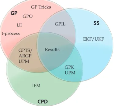
In this thesis we develop advanced methods for temporal data. We compare our methodology to the standard linear approaches such as autoregressive (AR), mov-ing average (MA), and Kalman filter methods as well some nonlinear extensions. TIM is a naive model that will serve as a reference point or “baseline” for per-formance. The bulk of the thesis’ material is found in three chapters: Gaussian processes, state space models, and change point detection. We summarize how each of these elements — Gaussian processes, state space, and change points — combine to form this thesis’ contribution in the Venn diagram of Figure 1.3.

In Chapter3, we give a brief introduction to Gaussian processes (GPs) before moving on to advanced aspects. Gaussian processes are a nonlinear regression method, extending (1.3), that do not assume the function underlying the rela-tionship between x and y can be represented by an analytic form. They belong to a class of methods known asBayesian nonparametrics. We review two ways of accounting for extra sources of uncertainty in GPs: uncertain inputs and output scale uncertainty. In uncertain inputs, the input variable x is known only up to a Gaussian distribution. We must “hedge our bets” when making predictions on the outputs y in that case. In output scale uncertainty we treat the scale, or units, of the outputs y as unknown and they must be inferred from data. This is sometimes known as a “t-process.” We make contributions by offering a sim-plified derivation of the uncertain input equations and presenting updates to do inference in the t-process for the same computational cost as a standard Gaussian process.

There are two approaches to applying Gaussian process methods to time series: Gaussian process time series (GPTS) and the autoregressive Gaussian process (ARGP). We compare these two approaches: The GPTS generalizes many of the

(28)

CPD SS GP IFM GPIL EKF/UKF GPO Results GPK UPM GPTS/ ARGP UPM GP Tricks UI t-process

Figure 1.3: A Venn diagram representing the contributions and topics in this thesis. We present the areas as change point detection (CPD) (Chapter 5), Gaussian processes (GP) (Chapter 3), and state space models (SS) (Chapter 4). Gaussian process optimization (GPO) (Section 4.2.1), GP uncertain inputs (UI) (Section 3.2), and uncertain output scale (the “t-process”) (Section 3.1) are in the GP circle. Gaussian process inference and learning (GPIL) (Section 4.3) is both Gaussian processes and state space modeling. Gaussian process change point models (Section 5.3) cover Gaussian processes and change point detection. Whereas, the independent factor model (IFM) is only in change point detection. Improvements to the unscented Kalman filter (UKF) (Section 4.2), and the re-lated EKF are in state space modeling. Finally, the results section (Section 5.5) evaluates methodologies in all circles.

standard linear time series methods, while the ARGP is arguably more general still than the GPTS. However, some elegant properties of the GPTS are lost when moving to an ARGP. The ARGP is also more computationally difficult than the GPTS. We review and extend methods to bring down the computational penalty of GPTS using Toeplitz methods or approaches that convert a GP to a Kalman filter (GPK). Rank-1 matrix updates bring down the cost of ARGP. We extend Rank-1 updates with a novel method called the sub-evidence that allows us to cheaply make predictions at any point in a time series for any starting point of

(29)

the training data.

Chapter 4 emphasizes state space models. We review existing work in state space models such as the Kalman filter. Approximate extensions designed for systems governed by nonlinear differential equations such as the extended Kalman filter (EKF) and unscented Kalman filter (UKF) are presented in a unifying framework for approximate filters. We cover some of the failure modes of these approximations, i.e. poor predictive performance, and introduce model based methods to make such failure less likely. We utilize GPs through the use of Gaussian process optimization (GPO) for learning in this setup. GPs are also used in a state-of-the-art nonlinear filter known as the GP assumed density filter (GP-ADF), which utilizes the uncertain input methodology covered in Chapter3. We extend the GP-ADF by learning the system dynamics, in effect the governing differential equations, of time series with the Gaussian process inference and learning (GPIL) algorithm. Like a GP in a regression context, the GPIL does not assume the system can be represented by an analytic form. We empirically benchmark these approaches.

Finally, in Chapter 5 we extend the change point detection framework first presented by Adams and MacKay [2007] and Fearnhead and Liu [2007]. In a change point detection framework, we phase out old training data that is detri-mental to the performance of an underlying model. In the absence of change points, we would expect more data to only increase the performance of an al-gorithm. We first build upon this approach for hyper-parameter learning. We learn from training data quantities that were previously set by hand: What is the hazard function, how often do change points occur? What is the prior of the underlying model, i.e. what kinds of changes typically happen at change point? In extension of the previous approaches that assumed TIM-like or simpler linear models as the underlying model, we “plug-in” the Gaussian process based meth-ods, GPTS and ARGP, as the underlying model. The computational complexity can be greatly reduced using the methods of Chapter3: Toeplitz methods, GPK, and the sub-evidence. We can do this in both a streaming way, as the data is coming in, and honing our inferences in retrospect by extending the methods of Fearnhead [2006]. Our final contribution is a method for supervised change point detection that uses labeled known change points in training. We also

(30)

in-corporate label noise on the change point labels. Finally, we evaluate all of our methods and the standard approaches (over ten methods in all) on six real world data sets. The data sets, summarized in Chapter 2, are environmental appli-cations (Whistler snowfall, Nile record, fish killer), biology (bee waggle dance), geological engineering (well log), and finance (industry portfolios).

Measuring performance Throughout the machine learning literature, and this thesis, methods are motivated by performance increases. Therefore, we must precisely define how we measure performance. For iid problems, we randomly take N data points from our data set and place them in the training set, while the remaining N0 are placed in the test set. The parameters of a method are set using the training set, while the predictive accuracy of a method is measured on the test set according to a loss function. For time series methods, we generally train on the firstT time steps and test on the remainingT0 time steps; it is more realistic to test a model’s ability to predict the future based on the past than vice-versa.

Consistent with rational decision making we consider the average loss over each data point, where the loss function L_{∈ Y × A →} _R measures the compat-ibility between the actual data point y and an action a _{∈ A}. The average loss over each test point is known as the empirical loss:

b L:= 1 N0 N0 X i=1 L(yi, ai). (1.4)

The hypothetical limiting case is known as the generalization error: _L:= limN0_→∞Lb.

We obtain actionsa from predictive probability distributionp(yi|xi) by minimiz-ing the expected loss,

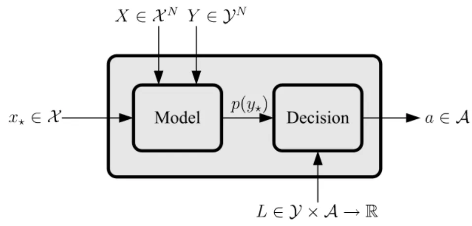
ai = argmin a E [L(yi, a)] = argmin a Z L(yi, a)p(yi|xi)dyi. (1.5) This procedure is known as Bayes’ decision rule. The black box functionality of a machine learning method is shown in Figure1.4.

(31)

Model Decision

Figure 1.4: Black box model of a machine learning algorithm. The algorithm is “configured” by a set of training inputs X and outputs Y. Then for any test input x? it outputs an action a. Inside the black box we have drawn two smaller black boxes which exist if a Bayesian decision process is being used. The first inner black box provides a predictive probability distribution p(y?) according to a model. The second inner black box implements (1.5).

L(yi, a) = (yi −a)2, and the mean-absolute-error (MAE), L(yi, a) = |yi −a|. The optimal actions for MSE and MAE are to assign a the mean and median of

p, respectively. We will also use the log loss, also called negative log likelihood (NLL), L(yi, p) = −logp(yi|xi), which has special properties for evaluating the entire predictive distribution p. More complex loss functions are possible for more complex tasks such as ranking, predictive intervals, resource allocation, and so on. A more thorough background and motivational aspects of performance evaluation is presented in Section B.1.

Bayesian machine learning Researchers in machine learning often borrow ideas from Bayesian statistics. A Bayesian approach allows us to apply the rules of probability in a unified way to the learning, prediction, and inference tasks. The probability of an event is treated as betting odds rather than a hypothesized limiting frequency in infinite independent trials (the frequentist paradigm). If we take probabilities to be betting odds, de Finetti [1931b] showed that the laws of probability are the unique rules that allow a bookie to avoid being placed in Dutch books: scenarios where a bookie takes a collection of bets where he will

(32)

lose money in every possible outcome.1 See Pollard [2002, Sec. 1.5] for details. In statistics, a common alternative to the Bayesian paradigm is hypothesis testing. Consider a celery detector in the fMRI example, for a Bayesian celery detector, we say the probability that the stimulus is a celery,given the image we observed, isx%. The analog of this statement in hypothesis testing (frequentist) terms would advertise that the probability of classifying the image as a celery stimulus given it is really from an airplane is less than α, usually 5% (this is known as a false positive rate). A practitioner would most likely use hypothesis testing for a model selector: The probability of observing some statistic of the data set, or more extreme in some sense, given it was actually generated from some proposed model where airplanes and celery give identical observations is less than 5%. We can illustrate the difference using an extreme case reasoning: A celery detector, or model selector, that completely ignored the data and randomly alerted 5% of the time would satisfy the frequentist statement.2

In machine learning, the generalization error is of primary importance. The frequentist optimality criterion here is the minimax risk: the “true” probability distribution of the data has been adversarially picked by nature to trick the algorithm. There is often no clear way to obtain the minimax optimal algorithm and bounds to the generalization error are often used as a proxy, for instance in Vapnik-Chervonenkis (VC) analysis [Vapnik and Chervonenkis, 1971]. This is in contrast to hypothesis testing; the statistical learning theory approach (such as VC analysis) emphasizes generalization error bounds. For any arbitrary sampling distribution, we could generate many independent data sets and only in less than 5% of them would the misclassification of airplanes and celery on the test set be more than . The bound can be calculated from the training set. A Bayesian machine learning algorithm has optimal Bayes’ risk: We get the lowest expected loss in expectation under the prior. A more in-depth coverage of these issues is in Section B.2.

1_{Websites such as}_{www.betfair.com}_and_{www.intrade.com}_{are modern manifestations of} the thought experiment inde Finetti[1931b]. If the odds available to those making simultaneous bets were notcoherent, i.e. consistent with the rules of probability, it would be possible to make a risk free profit through arbitrage.

2_{The concept of statistical power was developed to exclude such tests. However, power will} be the function of a true latent parameter. Only in simple situations will there be a test that is uniformly most powerful: more powerful than other tests for all values of a latent parameter.

(33)

1.2 Nonparametric Methods

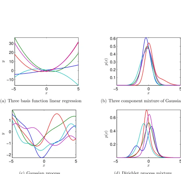
Nonparametric methods allow the number of parameters to grow with the sam-ple to better fit the data.1 _{In Bayesian methods, we must specify a prior on the} parameters before we observe the data, or even the sample size, which precludes us from changing the number of parameters as the sample size grows. Ferguson [1973] observed that the solution to this dilemma is for nonparametric Bayesian methods to place priors directly on infinite dimensional objects. We must make the “parameters” θ infinite dimensional.2 For instance, they can be functions (_RD _→ _R) as in Gaussian processes, over probability distributions M(_RD) as in Dirichlet processes (DPs), or over infinite binary matrices (_N_×_N _{→ {}0,1_}) as in the Indian buffet process. A corollary of the parameters θ being infinite dimensional is that the data cannot be summarized by any bounded finite num-ber of sufficient statistics as the data set grows. In fact, Hipp [1974] showed that only finite dimensional exponential family models summarize the data with sufficient statistics of bounded dimension. In other words, when making predic-tions we need to keep all the training data in memory; we cannot summarize the data by its sample mean and variance as in the parametric Gaussian case, i.e. TIM. We illustrate the more complex distributions that can be expressed by a nonparametric approach in Figure1.5.

Nonparametric methods are often motivated by making some set of param-eters in a parametric model infinite. For instance, Gaussian processes can be motivated as Bayesian linear regression with an infinite number of basis func-tions. Likewise, Dirichlet process mixtures (DPMs) are motivated as mixture models where the number of mixture components M become infinite. Paradox-ically, this often makes the algorithms more efficient. This is often because the computational complexity _O(_·) of a parametric (finite) model contains the num-ber of components M. Using nonparametric methods forces the modeler to use an efficient representation that is invariant to M since doing otherwise would

1_{In “All of Nonparametric Statistics”}_Wasserman_[₂₀₀₆_{, Ch. 1] infamously does not define} nonparametric statistics as to avoid inviting controversy. We take a more bold approach.

2_{The term nonparametric causes quite a deal of confusion as it often leads people to believe} we are working with models with zero parameters when in fact we are referring to models with an infinite number of parameters!

(34)

cause the computational complexity to become infinite when working with the nonparametric version.

A common question to ask is whether nonparametric models offer any ad-vantage over their parametric counterparts when the number of components M

is relatively large. In the nonparametric model the number of parameters (infi-nite) is always much larger than the number of data points; in the parametric case, there is alwayssome data setN where the parameters no longer outnumber the data points. Realistically, we may never reach that regime. However, recall Ferguson [1973] noted that in a perfectly coherent Bayesian setting the number of data points N should not affect our model choice. Often, it is merely more elegant to let the number of parameters become infinite than pick some large, but still arbitrary, number.

(35)

−5 0 5 −10 0 10 20 30 x y

(a) Three basis function linear regression

−5 0 5 0.1 0.2 0.3 0.4 0.5 0.6 x p ( x )

(b) Three component mixture of Gaussians

−5 0 5 −2 −1 0 1 x y (c) Gaussian process −5 0 5 0.2 0.4 0.6 x p ( x )

(d) Dirichlet process mixture

Figure 1.5: Sample draws illustrating the difference between nonparametric and parametric distributions. The top row shows parametric models while the bottom row shows their nonparametric extension. The left column is for regression while the right column is density estimation.

(36)

1.3 Overview of Time Series Data

In this section we describe the time series data paradigm, challenges in modeling real world time series, and the two main modeling approaches. All probabilis-tic time series models are based on either the autoregressive or the state space approach (known as data driven and parameter driven models, respectively, in econometrics [Francis et al., 2011]). Accounting for many aspects of real world time series, such as periodicity and missing data, is an often ignored part of the literature, but is important in application. We build on this section’s introduc-tion to the autoregressive approach in Chapter3. Likewise, we build on the state space approach in Chapter 4.

Time series are quantities that vary through time. They often consist of continuous measurementsytthat can be sampled at any point in time, arbitrarily. Examples include circuit voltage, atmospheric temperature, and stock market returns. In more precise terms, time series data maps from a time indext_{∈ T} to a measurementyt∈R. Time series can be in discrete time (T =Z) or continuous time (_T = _R), meaning discrete time is a special case of continuous time. For example, if we measure the voltage exactly once per hour we model it as discrete time where the time index is how many samples have been taken so far. We call this caseuniform sampling. However, if voltages are measured at arbitrary times or with changing sampling rates it is more convenient to model it as a continuous time process. To simplify the analysis we often, but not always, focus on discrete time processes.

If we are looking at multivariate time series, for example if we are considering a circuit’s voltage and current in the same model, then it is easier if we have

synchronized sampling. The sampling is synchronized if the different quantities, also referred to as channels, are sampled at the same time. In the multivariate case, y_t _∈ _RD_{, we treat a time series as discrete if the sampling is uniform and} synchronized. Otherwise, it makes more sense to use continuous time models. Note that discrete time still allows for missing data. If the data is sampled at one minute intervals but occasionally there are two or three minute gaps between data points then we model it as discrete time with missing data.

(37)

Model Decision Memory

Figure 1.6: Black box model of a time series method. This is the temporal analog to the iid black box in Figure 1.4. The model is the same as in the earlier iid black box except we now have a memory unit drawn on the bottom of the model. This signifies that information from recent data points is stored for predictions. The time series comes in one step at a time in yt along with its external inputs, also known ascovariates orcontrol inputs, xt.

1.3.1 Challenges in Time Series Data

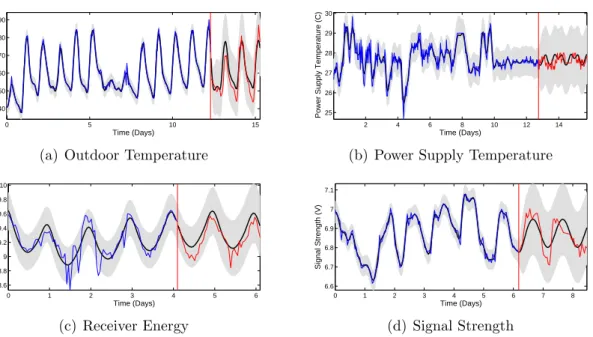
Throughout this thesis we discuss approaches to handling features often found in real world time series. In this section we give an overview of the challenges often present. These challenges are often ignored since they are not theoretically interesting, and are therefore under emphasized. However, we motivate aspects of the models constructed in later chapters based on these ideas. Furthermore, we take these challenges into consideration during the evaluation of the methods. The challenges in this section are illustrated on a real example in Figure 1.7.

Trends The most common time series feature to account for is trends. For instance, if there is a clear linear trend in the time series, it is inadvisable to use a model that aggressively reverts to the mean when extrapolating. However, simple linear models are even worse for extrapolating as they assume a time series will keep increasing or decreasing forever. Trends can also be removed through differencing. Exponential trends can sometimes be elegantly handled by moving

(38)

0 5 10 15 40 50 60 70 80 90 Time (Days) Outside Temperature (F)

(a) Outdoor Temperature

2 4 6 8 10 12 14 25 26 27 28 29 30 Time (Days)

Power Supply Temperature (C)

(b) Power Supply Temperature

0 1 2 3 4 5 6 8.6 8.8 9 9.2 9.4 9.6 9.8 10 Time (Days) Rx Eb/No (dB) (c) Receiver Energy 0 1 2 3 4 5 6 7 8 6.6 6.7 6.8 6.9 7 7.1 Time (Days) Signal Strength (V) (d) Signal Strength

Figure 1.7: We illustrate some of the challenges of real time series data on four examples from an electronic communication system. In each of the figures, the blue line represents the time series in the past while the red line represents it in the future. The black line and gray region represent the mean and 95% error bars in an example time series analysis on each time series; The region after the vertical red line is a forecast based on the data before the red line. Periodicity, at a daily period, is present to some degree in all the examples. Likewise, all the time series have some degree of a smooth underlying pattern, a short term correlation, not explained by the periodicity. The outside temperature and power supply temperature show obvious change points. The power supply temperature is visibly discretized to 1 C levels.

to the “return” space:

rt := log yt yt−1 = log(yt)−log(yt−1). (1.6)

The term return space is used as this formula converts between prices and returns when working with financial data. Using Gaussian process methods, covered in Chapter 3, the model can automatically and implicitly difference, or move to return space, time series when appropriate. We can strike an appropriate balance between aggressive extrapolation and mean reversion in a model based manner.

(39)

Gaussian noise then the noise variance in yt−yt−1 is twice that in yt. However, there is no loss in information as differencing is an invertible operation. A model on the differenced time series merely implies a different model on the original time series. We can work with the differencing level that is most compatible with a given model. Therefore, although differencing increases the “noise level” differencing does not necessarily lower performance.

Periodicity Many real world time series involve periodic patterns, especially on natural time scales, such as days, weeks, or years. A common approach to periodicity is to look at the Fourier transform of the time series and find frequen-cies with large power. Sinusoids at this frequency are then removed (band-pass filtering) [Baxter and King,1999]; however, this requires setting arbitrary thresh-olds. Differencing over the time of a period can also be applied. These ad hoc approaches can introduce artifacts and be counter-productive [Nelson and Kang, 1981]. In Chapter 3 we illustrate how model based approaches to handle peri-odicity are more elegant and effective. If the periperi-odicity occurs in multiplicative fashion, preprocessing with a log-scale transform can be useful.

Outliers Outliers could be the result of an unusual effect in the actual pro-cess being observed. Financial returns are notorious for being “heavy tailed” and many traders have been ruined for making erroneous Gaussian assumptions [Crouhy et al., 2005, Ch. 14]. However, the outliers in question may simply be “junk data.” For instance, missing data may be mistakenly entered as a mea-surement of zero due to careless programming. Outliers may also be the result of sensor anomalies, where a sensor gets stuck at a certain value. Machine learning methods for sensor failure detection were explored inOsborne et al. [2010].

Standardizing In general, it is advisable to standardize (linearly transform the data y_1:_T to have mean zero and unit variance) a time series before applying a method to it. Firstly, it may help if a method is not appropriately scale invariant. Additionally, standardization may alleviate numerical problems. Data whitening [Bishop, 2007, Ch. 12] can be applied to multivariate data to make each channel uncorrelated.

(40)

Standardizing allows the data to subtly influence the prior, which is illegal in a strict Bayesian formalism. In other words, standardizing induces a data dependent prior. For instance, placing the mean of the prior of the data at zero and then standardizing the data is the same as placing the prior at the sample mean of the data.

If we are willing to learn the mean by maximum likelihood anyway then standardizing does nothing more than avoid potential numerical problems. If we are trying to do full Bayesian inference, standardizing the data will usually only give the prior a small peek at the data and make little difference to the resulting inferences. However, recent developments suggest this is not always the case in nonparametric models such as Dirichlet process mixtures [Darnieder, 2011].

If the training set is continuously growing, we want our methods to learn the scale of the data. They should be robust enough to work without any standard-izing. However, we can standardize the data to some initial estimate of the scale of the data anyway, to limit the potential for numerical difficulties.

Short-term correlations Short-term correlations can be visualized by auto-correlation functions (ACF), partial ACFs (PACF), and scatter plots. The ACF on a time series y_1:_T is defined as:

ACF(p) := Corr [yt, yt−p] =

Cov [yt, yt−p]

p

Var [yt] Var [yt−p]

, (1.7)

and the PACF is:

PACF(p) := Corryt, yt−p|yt−p+1:t−1 (1.8) = Cov yt, yt−p|yt−p+1:t−1 q Varyt|yt−p+1:t−1 Varyt−p|yt−p+1:t−1 . (1.9)

The methods of Chapter 3 fit “hand-in-glove” for directly modeling short-term correlations.

(41)

Change points Parameters in the generative process may suddenly change. Typically we would expect that the more data is observed the better a model will perform at predicting. However, in time series analysis there are times in practice where using old data is counter-productive. Many ad hoc approaches [Anagnos-topoulos et al.,2008] have been developed to throw away old data, most of which involve placing some form of “forgetting factor” in a parameter estimator to im-plement a Robbins-Monro like scheme [Robbins and Monro,1951]. The methods in Chapter5automatically phase old data out as it becomes less accurate in mak-ing predictions. Such change points methods work in a fully coherent Bayesian manner without resorting to approximate inference.

Missing data Missing data is the source of many real data statistical headaches. Substituting zero or some other value for missing data is a naive, yet sometimes used method. An advantage of a fully probabilistic approach is that it allows for a principled way to deal with missing data. A missing variable is simply marginal-ized out instead of conditioned on. A matter of concern is themissing at random

assumption [Little and Rubin, 1987]. Does observing the data point as missing provide information of its latent value? This issue arose in the NetFlix challenge and was studied by Marlin et al. [2007]. When NetFlix users are rating movies, the fact that they have not rated a movie means they have decided not to watch it. Contrary to the missing at random assumption, this provides information that they may not rate the movie highly. We emphasize the distinction between the

observation that data is missing and theassumption that it is missing at random.

Censored data Sensors often have minimum and maximum values that are sometimes exceeded in the data. For instance, a thermometer might only return data in a range of 0 C to 100 C. Properly modeling the observation using P(x_≥

100) may give much different results than p(x= 100).

Discretization Sensor data is often coarsely discretized to ∆x intervals. A sensor might be designed to only report as many significant digits as it is confi-dent in. For instance, a thermometer might only report to the nearest ∆x= 1 C. Numerical and other problems can result when applying a method that expects

(42)

the data to be continuous to discrete data. For instance, a long stream of iden-tical measurements x, which should not happen in continuous data, may cause problems when attempting to infer the variance.

The most principled approach is to consider the latent value of the continuous time series prior to discretization xcont

t , which is within a certain range of the observed discretized value xt. Meaning we work with P(xcontt ∈[xt−∆x/2, xt+ ∆x/2]) rather than p(xcont

t =xt). We can also add a minimum noise level in the model according to the discretization level ∆x. However, a simple fix that works with any black box method, is to add salt to the data x to arrive at salted data

s:

st :=xt+t, t∼ U[−∆x/2,∆x/2]. (1.10) The more rigorous approach would be to create many salted versions of a train-ing set and average the predictions. However, a strain-ingly salted method may give approximately the same answer if the added noise is very small relative to the signal.

We justify salt by the following setup. Suppose we are given a black box that computes p(θ_|xcont

1:T ), possibly the posterior on some parameters or a posterior predictive. However, since we only have x1:T we must use this black box to compute p(θ_|x1:T). We see that

p(θ_|x1:T) =

Z

p(θ_|xcont_1:_T )p(xcont_1:_T _|x1:T)dxcont1:T , (1.11) p(xcont_1:_T _|x1:T)∝P(x1:T|xcont1:T )p(x cont 1:T ) (1.12) (1.10) = p(xcont_1:_T ) T Y t=1 I{xcontt ∈[xt−∆x/2, xt+ ∆x/2]}. (1.13)

If ∆xis small enough such that the prior predictivep(xcont

1:T ) is approximately con-stant within the small region near x1:T then the posterior will be approximately

(43)

uniform: p(θ_|x1:T)≈ Z p(θ_|xcont_1:_T ) T Y t=1 U[xcont_t _{| −}∆xt/2,∆xt/2]dxcont1:T (1.14) ≈ 1 N N X i=1 p(θ_|si_1:_T), (1.15) where si

t is the ith out of N iid draw of st from (1.10). We arrive at the salted algorithm by averaging over many salted versions, which effectively reduces the variance from Monte Carlo error in (1.10).

Non-uniform sampling Data analysis is simplest when a sensor is sampled on a periodic interval, e.g. exactly every 600 s. Uniform sampling makes the data naturally suited towards discrete time methods. However, this is not always the case in real world data, which gives an advantage to time series methods that work in the continuous time domain.

Point masses Point probability masses often occur in what might be assumed as a continuous variable. For instance, we could treat daily snowfall as a contin-uous variable with a smooth density. However, there is a positive probability of seeing exactly 0 cm of snowfall in a day. In this case, we might want to use a clas-sifier to estimate the probability that it snows paired with a regression method to predict the log snowfall conditional that it does snow.

Summary This description of challenges is by no means exhaustive, but should have sufficient coverage. Details of certain challenges given an emphasis in this thesis are: periodicity, short-term correlations, and change points. Discretization is present to some degree in all data sets. Discretization is often, but not always, neglected. In later chapters, we discuss continuous time models that can handle non-uniform sampling without difficulty. These challenges provide a context for other parts of the thesis.

Much of the literature on these challenges in machine learning is augmented by similar literature in signal processing, for instance: censored data [Olofsson, 2005], a review of the long studied connection between the ACF/PACF and the

(44)

frequency domain [Oppenheim and Schafer, 1989], a review of “robust” signal processing for handling outliers [Kassam and Poor, 1985], extensions to non-uniform sampling [Marvasti,2001], and handling missing data [Cooke et al.,2001].

1.3.2 Modeling Approaches

Discrete time data is modeled using either autoregressive or state space ap-proaches. State space models are based on the notion that there is an unobserved true state of the system, or latent state, evolving over time that can only be ob-served indirectly. For example, the location of a car can only be obob-served through noisy observations from either an odometer or a GPS. Tracking and control as well as unsupervised tasks like visualization or time dependent dimensionality reduction depend on the notion of a state space. Other applications, such as finance, are more interested in predicting future observations than finding the latent state. There, the latent state is merely a tool, which may or may not be beneficial for prediction.

The most basic state space model with continuous valued latent state is the linear dynamical system (LDS), which is the discrete time analog of a linear differ-ential equation. The hidden Markov model (HMM) [Baker, 1975] is the discrete space analog of an LDS. LDS methods treat predictable nonlinear behavior as noise to a large degree. Many approaches have been invented to make predictions in nonlinear dynamical systems (NLDS), Section 4.1.3.

To make the state space/autoregressive dichotomy concrete, suppose we have a time series of length T, Y := [y₁, . . . ,y_T]. In an autoregressive approach we directly model the function mapping the last p values1 _of _y _{to the next value of} y. A model of the form:

y_t _∼p(y_t_|Y(p), θ) (1.16)

is an autoregressive model of order p with parameters θ. We typically restrict

1 _{We use the shorthand of (}_N_{) := (}_t

−N):(t₋1) for the last N elements before a time indext.

(45)

(a) Autoregressive model (b) State space model

Figure 1.8: Graphical models for autoregressive and state space models. The autoregressive model shown here happens to be of order two. These graphical models show the difference in conditional independence assumptions between the two approaches. The dark blue shading signifies an observed node (variable) while the light blue signifies a latent variable.

ourselves to consider the case where:

p(y_t_|Y(p), θ) =N(f(Y(p)),Σ), (1.17)

for some function f _∈_RD×p _→ _RD and noise covariance Σ _∈_SD. By contrast, a state space model would be of the form:

xt∼pf(xt−1|θ), yt∼pg(xt|θ), (1.18) where typically onlyy_t is directly observable. Similar to the autoregressive case, we typically restrict ourselves to consider the case where:

pf(xt|xt−1, θ) =N(f(xt−1),Σf), pg(yt|xt, θ) = N(g(xt),Σg), (1.19) where f _∈ _RD _→

RD and Σf ∈ SD are the system function and system noise covariance, respectively. Likewise, g _∈ _RM _→

RD and Σg ∈SM are the

observa-tion funcobserva-tion andobservation noise covariance, respectively. If we further restrict ourselves to linear systems we are left with the form:

xt∼ N(Axt−1,Σf), y_t_{∼ N}(Cxt,Σg).

(1.20)

Some draws from systems (1.17) and (1.18) are shown in Figure 1.8.

(46)

(POE).1 If we summarize our prior on the model as p(θ), we summarize the autoregressive form as:

p(Y, θ) = p(θ) T

Y

t=1

p(y_t_|Y(p), θ). (1.21)

Where as in the state space form:

p(X,Y, θ) = p(θ) T

Y

t=1

p(y_t_|xt, θ)p(xt|xt−1, θ). (1.22)

In the case of nonparametric models θ might be infinite dimensional and we cannot work with p(θ) explicitly, as mentioned in 1.2, requiring us to write the POE after integrating out θ. For the autoregressive model this is:

p(Y) = T

Y

t=1

p(y_t_|Y1:t−1), (1.23)

which is merely the standard one-step-ahead predictive formulation of the marginal likelihood p(Y), also known as the evidence. For the state space model:

p(X,Y) = T

Y

t=1

p(y_t_|X1:t,Y1:t−1)p(xt|X1:t−1). (1.24)

Both of these reductions are merely using the marginalization rules of probability.

We can convert between modeling data y_t in autoregressive or in state space form. Just as we integrate outθ from the state space form to get (1.24), we can further marginalize outxt from a state space model leaving us with a predictor in autoregressive form (1.23), albeit with potentially infinite order. In practice, we may predict with the marginals of bounded order p(y_t_|Y(p)) instead of using all

the informationp(y_t_|Y1:t−1). We can approximate a state space model via a finite

order autoregressive model. If we are using the negative log likelihood (NLL) as the loss measure, we quantify the loss in predictive accuracy from truncating the

(47)

model order using mutual information:

I(y_t;Y1:t−p−1|Y(p)) (A.43)

= H[y_t_|Y1:t−p−1]−H[yt|Y1:t−1] (1.25) (A.45)

= _E[NLL under order pmodel]₋_E[NLL under state space model] . (1.26) This quantifies how much information is thrown away by discarding Y1:t−p−1

when making predictions.

Alternatively, we convert an autoregressive model into a state space form by “storing” the previous observations in the latent space. We use the following setup:

yt=xt,1 ∈R, xt,1 ∼p(xt−1,1:p|θ), xt,i =xt−1,i−1, i∈2:p , (1.27)

where p is the autoregressive predictor from (1.16) substituting xt−1,1:p for y(p).

Therefore, a state space model with latent dimension D=p_×E would be more generic than an autoregressive model of order p.

The distinction of state space models and autoregressive models provides a good first level splitting in the taxonomy of time series methods. In physical systems, prior knowledge often tempts the use of state space models. Knowledge of the equations of motion, for example, makes the representation of a state space model much more natural. State space models also have the advantage of not requiring the specification of an arbitrary order parameter. However, when inference becomes difficult the direct approach of autoregressive models can be advantageous.

1.3.3 Online Algorithms

Many applications demand online algorithms, meaning they are able to incor-porate a new data point without repeating the entire training procedure. More generally an offline algorithm is known as a batch method.

In the state space community, online and retrospective inference tasks are known as filtering and smoothing, respectively. We consider the case of a

(48)

ve-hicle tracking system to illustrate the distinction. When we are designing an autonomous navigation system; we would like to perform filtering. The system must decide where to steer the vehicle next based on its current location. The system must use the latest information from its sensors to detect oncoming obsta-cles. By contrast, a system on a Google street view1 _{car is capable of smoothing.} Street view must tag GPS locations to the street view photographs before being used. The street view system uses GPS and odometer measurements taken be-fore and after the photo was taken. Street view has the luxury of using past and future GPS information in a retrospective context.

A subset of online methods is stream processing methods; these methods not only update to new points but do not have to keep the previously observed data in memory. These methods are memory efficient since they only need to keep

sufficient statistics of the data.

Summary We have discussed the two different approaches to time series mod-els: autoregressive and state space. In each framework we can use either linear or nonlinear models. Most of the classical methods are linear, but may struggle to fully account for the common features in time series discussed. Methodology in Chapter 3 covers nonlinear versions of autoregressive models and Chapter 4 covers nonlinear versions of state space models. Both chapters embrace a non-parametric Bayesian approach. These extensions help us deal with the frequent time series challenges, periodicity, change points, non-uniform sampling, etc., in a principled manner.

(49)

Chapter 2 Data Sets

In this chapter we provide a preview of the data sets used in the experimental results, Section1.3.1. This provides a context in which to view the methodological developments in the following chapters. We use six real data sets: Nile, well log, snowfall, bee dance, industry portfolios, and “fish killer.” These data sets vary greatly in size and dimensionality. They each contain different aspects of time series mentioned in Section5.5. We aim to best visualize each of the data sets to assist in noticing each of these time series features. We summarize the data sets used throughout this thesis in Table 2.1. Additionally, we provide the source of each data set in Table 2.2.

Name T domain units SF US SS labels

Nile 663 _R+ _mm _{1 year} _Yes _N/A _No

Well Log 4,050 _R+ - - Yes N/A No

Snowfall 13,880 _R+ _cm _{1 day} _Yes _N/A _No

Bee Dance 4,960 _R2_×_[0_,₂_π_] _{px px rad} _{1/15 s} _Yes _Yes _Yes

Portfolios 11,455 (_R+)30 USD 1 day No Yes No Fish Killer 45,175 _R+ _m _{15 min} _Yes _N/A _Yes

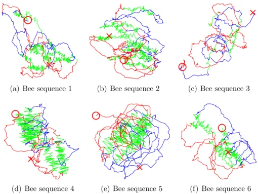
Table 2.1: Summary of data sets used. Sampling frequency is abbreviated as SF, while uniform sampling is abbreviated as US, and synchronized sampling as SS. The US dollar is abbreviated as USD. The bee data is made up of six sequences of length: 1,057, 1,124, 602, 756, 813, and 608. This gives a total of 4,960 frames. The x and y coordinates are measured in pixels (px) while the angle is radians (rad).

(50)

Name Source

Nile http://lib.stat.cmu.edu/S/beran

http://mldata.org/repository/data/viewslug/nile-water-level/ Well Log Schlumberger

http://mldata.org/repository/data/viewslug/well-log/ Snowfall http://www.climate.weatheroffice.ec.gc.ca/

Whistler Roundhouse station, identifier 1108906 http://mldata.org/repository/data/viewslug/ whistler-daily-snowfall/

Bee Dance http://www.cc.gatech.edu/~borg/ijcv_psslds/ http://mldata.org/repository/data/viewslug/bee/

Portfolios http://mba.tuck.dartmouth.edu/pages/faculty/ken.french/Data_ Library/det_30_ind_port.html

http://mldata.org/repository/data/viewslug/industry-portfolio/ Fish Killer Aquatic Informatics

http://mldata.org/repository/data/viewslug/fish_killer/

Table 2.2: Sources of data sets used. We summarize the original source of each data set used. We also provide the location of the data set on the http: //mldata.org/ data set repository.

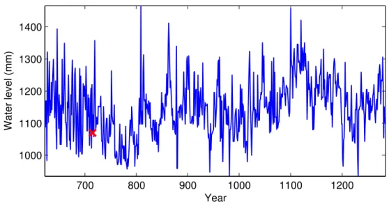
Nile data We consider the Nile data set [Beran,1994], which has been used to evaluate many change point methods [Garnett et al.,2009;Whitcher et al.,1998]. The data set, shown in Figure 2.1, is a record of the lowest annual water levels on the Nile river during 622–1284 measured at the island of Roda, near Cairo, Egypt. Domain knowledge in geophysics suggests a change point in year 715 due to an upgrade in ancient sensor technology to the nilometer. Eltahir and Wang [1999] provides evidence that anomalies in the Nile record can be used to infer years of El Ni˜no. The installation of the nilometer is the most visually noticeable change in the time series.

Bee waggle dance data Honey bees perform what is known as a waggle dance on honeycombs. The three stage dance is used to communicate with other honey bees about the location of pollen and water. Ethologists are interested in iden-tifying the change point from one stage to another to further decode the signals bees send to one another. The bee data set contains six videos of sequences of bee waggle dances [Oh et al.,2008]. The video files have been preprocessed to extract the bee’s position and head-angle at each frame, which is shown in Figure 2.2. While many in the literature have looked at the cosine and sine of the angle, we