R E S E A R C H
Open Access
A Bayesian robust Kalman smoothing
framework for state-space models with
uncertain noise statistics
Roozbeh Dehghannasiri
*, Xiaoning Qian and Edward R. Dougherty
Abstract
The classical Kalman smoother recursively estimates states over a finite time window using all observations in the window. In this paper, we assume that the parameters characterizing the second-order statistics of process and observation noise are unknown and propose an optimal Bayesian Kalman smoother (OBKS) to obtain smoothed estimates that are optimal relative to the posterior distribution of the unknown noise parameters. The method uses a Bayesian innovation process and a posterior-based Bayesian orthogonality principle. The optimal Bayesian Kalman smoother possesses the same forward-backward structure as that of the ordinary Kalman smoother with the ordinary noise statistics replaced by their effective counterparts. In the first step, the posterior effective noise statistics are computed. Then, using the obtained effective noise statistics, the optimal Bayesian Kalman filter is run in the forward direction over the window of observations. The Bayesian smoothed estimates are obtained in the backward step. We validate the performance of the proposed robust smoother in the target tracking and gene regulatory network inference problems.
Keywords: Kalman smoother, Robust filtering, Bayesian robustness, Innovation process, Orthogonality principle
1 Introduction
Classical Kalman filtering is defined via a set of equations that provide a recursive evaluation of the optimal lin-ear filter output to incorporate new observations [1]. The filtering procedure assumes a state-space model consist-ing of a transition equation and an observation equation. There are three filtering paradigms [2]: the Kalman fil-ter estimates the signal at the most recent observed time point, the Kalman predictor estimates the signal at a future time point, and the Kalman smoother estimates the signal at an intermediate observation time point. The equations for the filter and predictor are closely related, so that solving one provides an immediate solution for the other, whereas the smoother requires further work.
The issue that concerns us here is how to proceed when the model is not fully known. Classically, a precondi-tion for optimal filtering is to have complete knowledge of the random process model; however, this assumption
*Correspondence:[email protected]
Department of Electrical and Computer Engineering, Texas A&M University, College Station, Texas 77843, USA
is not always realistic in many practical settings such as target tracking [3–7]. Over the years, various adaptive procedures have been developed that essentially provide improving model estimates with increasing numbers of observations [8,9]. More recently, the problem has been addressed under the assumption that the model belongs to an uncertainty class of models governed by a prior proba-bility distribution, thereby placing the matter in a Bayesian framework with the aim being to find a recursive filter that is optimal over the uncertainty class.
There are two existing viewpoints for designing robust filters: minimax robustness, which involves designing a filter with the best worst-case performance [10–12], and Bayesian robustness, which involves designing a robust fil-ter with the optimal performance on average relative to a prior (or posterior) distribution governing the uncertainty class [13–16]. When designing a Bayesian robust filter, if optimization is not constrained, meaning that it is over the entire class of filters of a particular type, then the fil-ter is called anintrinsically Bayesian robust filter when optimality is relative to the prior distribution, and called anoptimal Bayesian filterwhen optimality is relative to
the posterior distribution. This kind of uncertainty mod-eling has been applied to linear and morphological filter-ing, both with and without incorporating the information embedded in the observations into the prior distribution [15,17]. In the case of Kalman filtering, the problem has been addressed for the filter and predictor without prior updating [16], which is called an intrinsically Bayesian robust Kalman filter, and with updating based on new data [18], which is called anoptimal Bayesian Kalman filter. In this paper, we find the optimal Kalman smoother relative to the probability mass governing the uncertainty.
In a Bayesian robustness setting, the prior (posterior) distribution is on the model of the underlying random process, meaning that it refers directly to our scien-tific uncertainty. The general aim is to find an operator that is optimal with respect to both the stochasticity in the nominal problem, for which the underlying model is fully known, and the model uncertainty. The aim can be achieved by replacing model characteristics and statis-tics in the solution to the nominal problem with their effective counterparts, which incorporate model uncer-tainty in such a way that the equation structure of the nominal solution is essentially preserved in the Bayesian robust solution. This approach has been used for classi-fication [19], linear and morphological filtering [15,17], signal compression [20], and Kalman filtering [16]. For example, in optimal wide-sense stationary linear filtering, the power spectra are replaced by effective power spec-tra [15] or in Gaussian classification, the class-conditional densities are replaced by effective class-conditional densities [19].
Anintrinsically Bayesian robust Kalman filter(IBR-KF) has been proposed in [16] that is optimal relative to the prior distribution of noise parameters. The theory of the IBR-KF is rooted in the Bayesian orthogonality principle and the Bayesian innovation process, which are the extended versions of their ordinary counterparts when applied to the prior distribution. Innovation pro-cesses have long been used for Kalman filtering, dating back to 1968 when Kailath proposed the first instance of an innovation-based approach for Kalman filtering [21]. Building on the IBR-KF theory developed in [16], an optimal Bayesian Kalman filter (OBKF) achieving opti-mality on average relative to the posterior distribution of the noise parameters when observations are incorporated into the prior distribution was proposed [18]. The OBKF shares the theoretical foundation of the IBR-KF, the differ-ence being the distribution relative to which the Bayesian innovation process and Bayesian orthogonality principle are stated. It is the prior distribution in the latter [16] and the posterior distribution in the former [18].
Kalman smoothing is an offline signal processing tool where both past and future observations are used for making estimations [22–29]. Kalman smoothers can be
classified as fixed-point, fixed-lag, and fixed-interval smoothers [30]; however, the term Kalman smoother gen-erally refers to the fixed-interval case in which the goal is to estimate the sequence of states over a finite time window using all observations in the same window.
In this paper, we assume that the parameters character-izing the second-order statistics of process and observa-tion noise are unknown and propose anoptimal Bayesian Kalman smoother(OBKS) framework to obtain smoothed estimates that are optimal relative to the posterior dis-tribution of the unknown noise parameters. Referring to our method as an “optimal Bayesian” smoother is consis-tent with the terminology used in other works devoted to the design of optimal Bayesian filters when a prior dis-tribution is assumed for the unknown parameters in the random process model [17,18].
In a sense, this paper fills in the last block of a six-part Kalman filtering paradigm: (1) filter/predictor under known model, (2) smoother under known model, (3) adaptive filter/predictor under unknown model, (4) adap-tive smoother under unknown model, (5) optimal fil-ter/predictor relative to an uncertainty class of models, and (6) optimal smoother relative to an uncertainty class of models. This is not to say that all problems have been solved. There can be many adaptive approaches. There are also many ways in which there can be uncertainty in the state-space model, and optimality relative to that uncertainty can be defined via different cost functions. In the four uncertainty settings referred to here, the covari-ance matrices for the process and observation noise are assumed to be unknown (in a manner to be precisely defined in the sequel).
two forward steps. In the first step, theposterior effective noise statisticsare computed. Then, the optimal Bayesian Kalman filter is designed relative to the obtained posterior effective noise statistics and is run in the forward direction over the window of observations. Finally, in the backward step, the Bayesian smoothed estimates are obtained.
This paper is organized as follows. In Section 2, we provide the theoretical foundation and derive the recur-sive equations for the proposed optimal Bayesian Kalman smoother. Section3is devoted to the experimental evalu-ation of the proposed OBKS method using two examples: target tracking and gene regulatory network inference. Finally, concluding remarks are given in Section4.
Here, we summarize the notations employed through-out the paper. We use uppercase and lowercase boldface letters to denote matrices and vectors, respectively.MT,
|M|, and Tr{M}represent the transpose, determinant, and trace (sum of diagonal elements) operators for matrix
M, respectively. Also, diag[·] represents the diagonal ele-ments of a diagonal matrix. The value of a time-dependent matrix at timekis denoted byMk. Let(P,,E)be a
prob-ability space, then E[·] denotes the expectation relative to the probability measureP. In a real-valued random vector
x=[x(1), ...,x(k)], each component is a real random vari-ablex(i): →R, 1≤i ≤k. We use E[x] and cov[x]= ExxT to denote the mean vector and the covariance matrix, respectively. Finally,N(x;μ,)denotes a multi-variate Gaussian function relative to random vectorxwith the mean vectorμand the covariance matrix.
2 Optimal Bayesian Kalman smoother
2.1 Problem formulation and theoretical background
In this paper, we consider the following parameterized state-space model:
the state vector and observation vector, respectively.k,
Hk, andk are matrices of sizen×n,m×n, andn×p
called the state transition matrix, observation transition matrix, and the process noise transition matrix, respec-tively. We letzθ1
vectors representing the process noise and observation noise, respectively, being zero-mean discrete white-noise processes. The unknown noise covariance matrices of the process and observation noise are given by
E
lection of all possible realizations for θ, governed by a prior distribution π(θ). We assume that θ1 and θ2 are
independent. Note that while the observation vector yθk
depends on bothθ1andθ2, the state vectorxθk1 depends
only onθ1.
Considering a state-space model according to (1) and (2) and an observation windowYLθ =yθ0,yθ1, ...,yθL of sizeL, we desire anoptimal Bayesian Kalman smoother(OBKS) that is a fixed-interval smoother involving finding the esti-mates of statesxθ1
0,x
θ1
1, ...,x
θ1
L in the same window. In this
context, the Bayesian smoothed estimatexθk|Lofxθ1
k , which
is the output of the OBKS at timek, has the following form
xθk|L=
L
l=0
Gk,lyθl, (5) such that the average MSE relative to the posterior distri-butionπθ|YLθis minimized: expectation relative to the prior distribution π(θ). Fur-thermore, E[θ] and Eθ|YLθrepresent the expectation of parameterθ relative toπ(θ) andπθ|YLθ, respectively. It is worth mentioning that the optimal Bayesian Kalman predictor and the optimal Bayesian Kalman filter pro-posed in [18] correspond toL = k−1 andL= kin (5), respectively. Also, if instead of Eθ∗[·], Eθ[·] is used in (6), the estimators corresponding toL = k−1 and L = k in (5) are called the intrinsically Bayesian robust Kalman predictor and filter, respectively [16].
Before developing the OBKS equations, we state a theorem and a lemma required for deriving equations whose proofs can be found in [16].
The next theorem is a restatement of the classical orthogonality principle relative to the inner product defined by Eθ∗[E[·] ] applied to xθ1
k , yθl, andxθk|L,
keep-ing in mind that xθ1
k depends only on θ1, whereas xθk
depends on θ =[θ1,θ2]. As originally stated in [16],
Theorem 1 (Bayesian Orthogonality Principle) The Bayesian smoothed estimate obtained in (5) satisfies (6) (having minimum average MSE relative to the posterior distribution) if and only if
Eθ∗ predictor at timek, then theBayesian innovation process is defined as [16]
zθk =yθk−Hkxθk|k−1. (8)
It can be shown that [16]
Eθ∗
is the Bayesian prediction error covariance matrix relative toθ. Note that ifzθ1
The following lemma, which can be proved similar to the proof given in [16], helps us find the Bayesian smoothed estimates using the Bayesian innovation pro-cess.
Lemma 1 (Bayesian Information Equivalence)The Bayesian smoothed estimatexθk|Lforxθk based upon obser-vations yθl, 0 ≤ l ≤ L, can be found by computing the Bayesian smoothed estimate based upon the Bayesian innovation processzθl,0≤l≤L.
2.2 Update equation for Bayesian smoothed estimate
We now proceed to develop the recursive structure of the OBKS based on the theoretical foundation laid out in the previous subsection.
Using Lemma1, we can have the following form for the Bayesian smoothed estimatexθk|Ldefined in (5):
xθk|L=
L
l=0
Gk,lzθl, (12)
wherexθk|L obtained in (12) should satisfy the Bayesian orthogonality principlerelative tozθl, forl≤L,
After some mathematical manipulations and also using (9), one can verify that
Gk,l=Eθ∗
Plugging (14) in (12) yields
xθk|L=
relative toθat timekand its auto-correlation E
due to the Bayesian orthogonality principle and vθ2
l is
independent fromxθk andxkθ|k−1 for k < l. Therefore, substituting (16), (15) becomes
Keeping in mind that we want to find a backward
recur-Considering (17) and (18), one can conclude that obtain-ing an update equation forxθk|Lrequires a recursive
rela-tionship between Eθ∗
is called theeffective Kalman gain matrix[18]. Also, we call Eθ∗Qθ1 and E
θ∗Rθ2 the posterior effective
pro-cess noise statisticsand theposterior effective observation noise statistics, respectively. As has been shown in [18], Eθ∗Qθ1is required for updating E
Using (22), we have
Eθ∗
where the second equality is obtained because, forl ≥ k, future process noiseuθ1
l and observation noisev
θ2
l are
independent fromxθk. Now plugging
Eθ∗
derived in [16], in (23) yields the following recursive equation for Eθ∗
where the second equality is obtained by multiplying E−θ∗1
is used to obtain the last equality.
Substituting (25) in (17) yields the update equation forxθk|L
as
where the third equality is obtained due to (18) and
Ak =Eθ∗
is called theeffective Kalman smoothing gain.
2.3 Update equation for the Bayesian smoothed error
covariance matrix Lettingxθk|L = xθ1
k −xθk|L be the Bayesian smoothed
xθk|L=xθ1 Taking the covariance matrix of both sides of (30) rela-tive to Eθ∗[E[·] ] yields
Due to the Bayesian orthogonality principle, for the left-hand side of (31),
Eθ∗
Similarly, regarding the right-hand side of (31),
Eθ∗
Thus, (31) can be simplified to
Eθ∗
Finally, (34) can be rearranged to obtain an update equation for Eθ∗
Finding the average Bayesian smoothing error covari-ance matrix in (35) completes all equations needed for implementing the OBKS framework.
The forward step of the OBKS involves running the OBKF and in the backward step the Bayesian smoothed estimates are obtained. We should point out that in prac-tice for the OBKF, the posterior effective noise statistics are updated sequentially for each k because filtering is an online estimation scheme. However, here since we use OBKF as the forward step of the OBKS, which is an offline estimation, we use the posterior effective noise statis-tics Eθ|YLθ relative to the whole observation window for the OBKF-based estimation from the beginning. In other words, the OBKF used in the forward step, is in fact
the IBR-KF designed relative to the posterior distribution
πθ|Yθ L
.
To better understand the similarity between the recur-sive structures of the proposed OBKS and the ordi-nary Kalman smoother, Table 1 compares the recursive equations required for these two smoothers. As this table suggests, the recursive structure of the proposed OBKS framework is similar to that of the classical Kalman smoother except that it employs effective characteristics, namely, the effective Kalman gain matrix Kk, effective Kalman smoothing gain matrix Ak, and the posterior effective noise statistics Eθ∗Qθ1and Eθ∗Rθ2.
If the state vector x0 is characterized by E[x0] and
cov[x0], then the forward step of the OBKS is initialized
as Eθ∗
2.4 Computing posterior effective noise statistics The forward step in the OBKS requires the posterior effective noise statistics Eθ∗Qθ1 and E
θ∗Rθ2. These
expectations should be computed relative to the poste-rior distributionπθ|YLθ. Since the closed-form solution
Table 1Comparison of the recursive equations for the classical and the proposed optimal Bayesian Kalman smoothers
of the distribution is not available, these expectations can be approximated via a Metropolis Hastings Markov chain Monte Carlo (MCMC) approach as proposed in [18]. To implement the MCMC method, we need to com-pute the likelihood function f YLθ|θ. Here, we outline the main steps needed to compute the likelihood func-tion and refer to [18] for more details. Taking into account the Markov assumptions in the state-space models, the likelihood function can be written as
f function for which we can use a sum-product algorithm called the factor graph [34]. Utilizing factor graphs, it can be seen that the likelihood function can be obtained as [18]
andL,ML, andSLare computed recursively utilizing the
following expressions fromk=0 tok=L−1:
wherekandWkare obtained as
k=
E[x0]. A pseudo-code outlining the computational steps
needed for computing the likelihood function is available in Additional file1.
The likelihood function fYLθ|θ is needed in a Metropolis Hastings MCMC method to decide whether the generated MCMC samples should be rejected or accepted into the sequence. In this MCMC method, a sequence of samples is generated sequentially where at each step, a new sampleθ(new)is generated based on the last accepted sample θ(old) according to a proposal dis-tributionf
θ(new)|θ(old). The new sampleθ(new)will be either accepted or rejected based on an acceptance ratior computed as follows: puted via the set of equations given in (39)–(46). The new sampleθ(new) will be accepted into the sequence of MCMC samples with probabilityr. Otherwise, it will be discarded and the last sampleθ(old)will be repeated in the sequence. When enough MCMC samples are generated, the posterior effective noise statistics Eθ|YLθare approx-imated as the average of the generated samples. When a symmetric proposal distribution, i.e.,f
θ(old)|θ(new) =
f
θ(new)|θ(old), such as a Gaussian distribution is used in our simulations, then (47) can be further simplified. Also, more explanation and a pseudo-code on how the recursive calculations in (42)–(46) should be performed are provided in Additional file1.
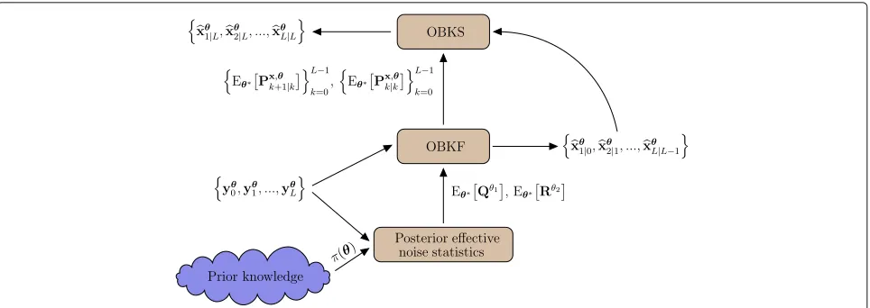
Fig. 1Illustrative view of the proposed OBKS framework. This figure presents the general framework of the proposed optimal Bayesian Kalman smoothing framework. The posterior effective noise statistics are obtained by integrating the data in the observations window into the prior distributionπ(θ), which are used to run the OBKF in the forward direction. Then, the Bayesian smoothed estimates are obtained in the backward direction as the outputs of the OBKS
the by-products of the OBKF in the forward direction. Also, all computational steps for the OBKS are sum-marized in Algorithm 1. The inputs are the prior dis-tribution, the matrices that characterize the state-space model, and the observations over the observation window.
Algorithm 1 Optimal Bayesian Kalman Smoother (OBKS)
1: input:π(θ),k,Hk,Qθ1,Rθ2,k,YLθ = {yθ0,yθ1, ...,yθL}
2: output:xθ0|L,xθ1|L,. . .,xθL|L 3: Eθ∗[Qθ1] , E
θ∗[Rθ2]←MCMC(Yθ
L,π(θ))
4:xθ0|0←E[x0]
5:xθ1|0←0E[x0]
6: Eθ∗P0x,|θ0←cov[x0]
7: Eθ∗P1x,|θ0←0cov[x0]T0 +0Eθ∗Qθ1cov[x
0]T0
8: fork=1, ...,Ldo 9: zθk ←yθk−Hkxθk|k−1
10: Kk ←EθPkx,|θk−1HTkEθ−∗1HkPkx|,θk−1HTk +Rθ2
11: xθk|k←xθk|k−1+Kkzθk 12: xθk+1|k ←kxkθ|k−1+kKkzθk 13: Eθ∗Pkx,|θk←(I−KkHk)Eθ∗Pkx,|θk−1 14: Eθ∗Px,θ
k+1|k
← kI−KkHk
Eθ∗
Pxk,|θk−1
T
k +kEθ∗Qθ1T
k
15: fork=L−1,L−2, ..., 0do 16: Ak ←Eθ∗Pxk,|θkTkE−θ∗1Pkx,+θ1|k
17: xθk|L←xθk|k+Akxθk+1|L−xθk+1|k 18: Eθ∗Pxk,|θL ← Eθ∗Pxk,|θk + Ak
Eθ∗
Pxk,+θ1|k
−Eθ∗
Pxk,+θ1|LAkT returnxθk|L
The outputs are the Bayesian smoothed estimates of the unknown states over the window obtained by the OBKS. There are four main steps in this algorithm. First, in line 3, the posterior effective noise statistics are estimated using the MCMC approach, as explained in Section 2.4, which are later used in the OBKF. Then, we need to initialize the OBKF as outlined in lines 4–7. Lines 8–14 are devoted to the OBKF, which is run in the forward direction. Finally, lines 15–18 show how the Bayesian smoothed estimates are obtained.
Also, in order to study the computational complexity of the proposed OBKS, since the proposed recursive struc-ture is completely similar to that of the ordinary Kalman smoother except using the posterior effective noise statis-tics, which are approximated using MCMC samples, we only need to analyze the complexity of the MCMC step. In the MCMC step, in order to obtain a sequence of MCMC samples, the likelihood function in (36) should be computed for each generated MCMC sample by iter-ating the equations given in (42)–(46) from k = 0 to k = L−1. Therefore, the dimensions of the state vector
xand the observation vectory, the size of the windowL, and the number of generated MCMC samples can affect the complexity. We should point out that some matrix calculations such as inversions, multiplications, and deter-minants might need to be performed only one time for each generated MCMC sample. For example, when the process noise covariance matrix is known and the system
is stationary, it is enough to computeTk
Qθ1
k
−1
once and then use it for the rest of the calculations.
3 Simulation results and discussion
matrix Pθk|,Lθ that characterizes the performance of the Kalman smoother designed by the assumption of θ =
θ
1,θ2
when applied to a model with the actual noise parametersθ =[θ1,θ2], which is given by [35] smoothing gain and Kalman gain matrices of the Kalman smoother and filter designed relative toθ, respectively, and matricesDθkandLθkcan be found recursively via
The initial conditions for these two matrices areDθL−1= KθLHLandLθ
L−1=Kθ
L−1HL−1.
We compare the OBKS with the steady-state minimax Kalman smoother, intrinsically Bayesian robust Kalman smoother (IBR-KS), and the model-specific Kalman smoothers designed relative to all possible values ofθ. The minimax Kalman smoother has the best worst-case per-formance among all possible model-specific smoothers and is defined by
θmm=arg min in the middle of the observation window, as the steady-state performance of a smoother occurs for the middle points in an observation window. The IBR-KS is simi-lar to the OBKS except that the optimization is relative to the prior distributionπ(θ). To design an IBR-KS, one can use the OBKS equations in Table 1 with expectations relative to the prior distribution rather than the poste-rior distribution. Therefore, for the IBR-KS the MCMC step is not needed. The IBR-KS approach provides optimal smoothing performance relative to the prior distribution.
3.1 Target tracking example
Let the dynamic of a vehicle at each time step be deter-mined by the state vectorxk =[pxvxpyvy]T, wherepx,vx,
py, andvyare the horizontal position, horizontal velocity,
vertical position, and vertical velocity, respectively. If the vehicle possesses a constant speed and the measurements are made with intervalsτ, then a state-space model with
the following matrices can characterize the dynamic of the vehicle at each time step [36–38]:
k =
The covariance matrices of the process noise and obser-vation noise are
whereqdetermines the process noise intensity. In the sim-ulations, we assume that the measurement interval isτ = 1 and the initial conditions are E[x0]=[ 100 10 30 −10]T
and cov[x0]=diag[ 25 2 25 2].
It is worth mentioning that when the process noise tran-sition matrixk is not an identity matrix, since the effect ofkon the Kalman equations is only through the covari-ance matrix of the process noise, a state-space model with the process noise covariance matrix Q and the process noise transition matrixk is equivalent to a state-space model with the process noise covariance matrix Qeqk =
kQTk and the process noise transition matrixkeq = I. With this in mind, we can consider the simulation results of the above target tracking example for an equivalent state-space model with the process noise transition matrix
k=
0.4719 0 0 0.8817
0 −0.8817 0.4719 0 0 0.4719 0.8817 0
⎤ ⎥ ⎥ ⎦,
and the covariance matrixQ = q×diag[ 0.0657 0.0657 1.2676 1.2676], where Q is the diagonal matrix of the eigenvalues andk is matrix of the eigenvectors forQ, i.e.,
Q = Q()T is the eigen-decomposition ofQ. There-fore, the simulations for the target tracking example can also be regarded for the case that the process noise transi-tion matrix is not an identity matrix.
various Kalman smoothing approaches. To do so, for a given sequence of observations YLθ, we find the error of each Kalman smoothing approach for eachkby first com-puting the error covariance matrix using (48), whereθ is replaced by Eθ|YLθ, E[θ], and θmm for the OBKS,
IBR-KS, and the minimax Kalman smoother, respectively, and then, the MSE at time k is obtained by finding the sum of diagonal elements of the error covariance matrix. The MSE for the optimal Kalman smoother designed relative to the actual θ value is obtained according to
Pk|L in Table 1. The reported average MSE is obtained
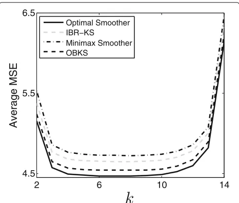
over 30 different assumed values of θ and 10 different observation sequences for each value (300 simulations in total). Figure2a presents the average MSE across the observation window obtained for each smoothing scheme. As can be seen, OBKS outperforms IBR and minimax approaches and its performance is close to the average of the optimal MSEs obtained by the optimal smoothers. Figure 2b shows the average MSE for the middle state (k = 8) in the observation window. In addition, this figure presents the average MSE of each model-specific Kalman smoother designed relative to value θ. Note that the difference between the definitions of the opti-mal smoother and the model-specific smoother is that the optimal smoother is designed relative toθ and always applied to model θ, but the model-specific smoother is designed relative to θ and then applied to the model
θ. This figure suggests the better performance of the OBKS compared to the IBR, minimax, and model-specific Kalman smoothers.
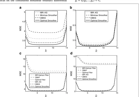
Figure 3a, b illustrate the performances of different Kalman smoothers for the observation noise variances
θ = 0.5 and θ = 4, respectively. Although θ is fixed, since the OBKS performance depends on the generated observations, we report the average MSE taken over 300
different generated observation sequencesYLθ. It can be seen that the OBKS has its performance close to the opti-mal Kalman smoothers and much better compared to other robust Kalman smoothers. Since the IBR approach is optimal on average relative to the prior distribution, not for each possible model within the class, it is not guar-anteed that the IBR-KS performs well for each model, an example being θ = 4 where minimax outperforms the IBR approach. However, even for models for which the IBR approach does not perform well, OBKS still gives promising results.
In Fig. 3c, d, in addition to the MSE values for dif-ferent smoothers, we also present the MSEs of various Kalman filters for each time step k. For different fil-ters, we compute Pθk|,kθ, as derived in [16], and report Tr0Pθk|k,θ1, whereθis replaced byθmm, E[θ], and E
θ|Yθ L
for the minimax, IBR, and OBKF approaches, respec-tively. Since the error covariance matrix of the filter is used as the initial value for the error covariance matrix of the corresponding smoother, fork = 15, the MSE of each smoother equals that of its corresponding filter. As expected, for other time indiceskwithin the observation window, the MSE of the smoother is always lower than that of the filter. Note that due to the range of they-axis in Fig.3c,d, the MSEs of various smoothing approaches might not be distinguishable. The difference between the performances of different smoothers is visible in Fig.3a,b.
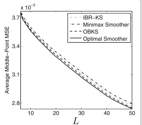
Next, we analyze the smoothing performance for different numbers of observations (observation window length) L. Figure 4 presents the average MSE of differ-ent Kalman smoothers at time stepL/2 (middle state) as L changes from 6 to 50. The average MSE for eachLis obtained in the same way as in Fig. 2. We can observe
a
b
a
b
c
d
Fig. 3Performance analysis of different smoothers for the target tracking example over the observation window.aMSE of different smoothers for
θ=0.5.bMSE of different smoothers forθ=4.cMSE of different smoothers and filters forθ=0.5.dMSE of different smoothers and filters forθ=4
Fig. 4Average middle-point MSE of different Kalman smoothers for different observation window lengthL
that when the number of observations is small, the per-formances of OBKS and IBR-KS are close because the expectation of θ relative to the posterior distribution is close to the expectation relative to the prior distribution; however, as the number of observations increases, the average MSE of the OBKS gets closer to that of the opti-mal smoothers because the expectation of the unknown parameter tends to the true parameter value. Moreover, both the OBKS and IBR-KS always outperform the mini-max Kalman smoother in terms of average MSE.
In the next set of simulations, we consider the case that both the process noise parameterqand the observation noise parameter rare unknown, being denoted by uni-form random variablesθ1andθ2over intervals [ 3, 5] and
[ 0.25, 5], respectively. Regarding the MCMC step, we use a multivariate Gaussian distribution with the mean vec-tor being the vecvec-tor of last accepted samples forθ1 and
θ2and a diagonal covariance matrix whose diagonal
and 10 different sets of observations for each pair of true values (2000 simulations in total) in Fig.5. As shown in the figure, the OBKS outperforms other robust smoothers and performs closely to the optimal smoother designed relative to the underlying true model.
In Fig. 6, we analyze the average MSE at k = 8, the middle point in the observation window. The white sur-face represents the average middle-point MSE for each model-specific Kalman smoother designed relative to the process noise parameterθ1 and observation noise param-eterθ2. We also show the average middle-point MSEs for the IBR-KS, minimax smoother, and OBKS, and the aver-age of the optimal middle-point MSEs obtained by the optimal smoothers by constant planes. This figure sug-gests that compared to other robust smoothers, the OBKS achieves the closest average middle-point MSE to that of the optimal smoothers.
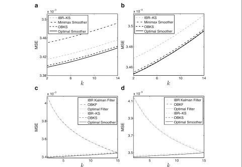
Figure 7 shows the performance of different smooth-ing approaches for two specific state-space models cor-responding to certain values of θ1 and θ2. Figure 7a, c
correspond to θ1 = 4.5 and θ2 = 1, respectively, and
Fig. 7b, dcorrespond toθ1 = 3.2 and θ2 = 4,
respec-tively. The figures in the first row report the MSE of different smoothers for each time instance within the observation window. For both state-space models, we see the promising performance of the OBKS. In addition to the MSEs of different smoothers, the second row gives the MSEs of different Kalman filters. The MSE of each smoother is initialized by the MSE of the corresponding filter, and then, it decreases as we proceed in the back-ward direction. The difference between the performances
Fig. 5Performance analysis over the observation window for the target tracking example with unknownrandq. Average MSE of different smoothers for eachkover the observation window when bothqandrare unknown
of different smoothers is visible in Fig.7a,b, which focus on a shorter range for the smoothing performance.
Figure 8 studies the effect of the size of the observa-tion window on the performances of different smoothing approaches. We vary the size of window L from 6 to 50 and report the average middle-point MSEs of various smoothers for eachL. WhenLis small, the performances of the OBKS and IBR-KS are close but as L increases, the performance of the OBKS tends to that of the opti-mal smoother. This is because the posterior effective noise statistics converge to the underlying true values as the number of observations increases.
In Fig. 9, we analyze the complexity of the proposed OBKS framework and how its runtime changes with the size of the window and the number of MCMC samples. We consider the target tracking example when the size of the window changes from 4 to 50 and the number S of generated MCMC samples is 5000, 10,000, and 15,000. Computations were performed on a machine with 16 GB RAM and Intel®CoreTMi7 2.5 GHz CPU. As can be seen, the run time tends to grow linearly withLandS. In our simulations, we set the number of samples in the MCMC step to 10,000 to obtain acceptable estimates at tolerable computational complexity.
Also, in Fig. 10, we study the effect of the number of MCMC samples, used to compute the posterior effec-tive noise statistics, on the OBKS performance. Similar to Fig.3a, we assume that the observation noise varianceθ is unknown and its true value is 0.5. We consider three different observation window sizes atL = 10, 15, 20 and vary the number of MCMC samples from 100 to 10,000. For eachLand number of MCMC samples, we report the middle-point MSE (MSE atk = L/2) over 300 different observation sequences generated based on the underlying true state-space model. As can be seen, as the number of MCMC samples increases (especially when the number of MCMC samples is not large enough), the OBKS per-formance gets better because more accurate posterior effective noise statistics can be obtained via more MCMC samples. However, after collecting enough MCMC sam-ples, the performance of the OBKS converges, and further increase of MCMC samples has little additional perfor-mance improvement. In our simulations throughout the paper, we used 10,000 MCMC samples.
3.2 Gene regulatory network inference
Fig. 6Average middle-point MSE of different Kalman smoothers for the target tracking example with unknownrandq. The average performance of each model-specific Kalman smoother corresponding to the noise parametersθ1andθ2is shown. The average MSE for the IBR-KS, minimax, OBKS, and the average of optimal MSEs are shown as constant planes
hidden states. Since acquiring exact knowledge of noise statistics is highly difficult due to the complexity of biolog-ical systems and other practbiolog-ical limitations, it is prudent to utilize a robust Kalman approach for inference. We focus on the continuous nonlinear ordinary differential
equation model [39], where the value of each genegi, 1≤
i≤n,nbeing the total number of genes in the network, is characterized as
˙
gi=ηi(g1, ...,gn)+vi,
a
b
c
d
Fig. 8Effect of the size of observations on the smoother performance in the target tracking example with unknownrandq
where g˙i, vi, and ηi(·) are the derivative of the
gene-expression value relative to the time variable, the exter-nal noise, and the regulatory function, respectively. The regulatory function ηi is a linear combination of some nonlinear terms [39]:
ηi(g1, ...,gn)=
Ni
j=1
[(αij+uij)ij(g1, ...,gn)] ,
whereNiis the number of nonlinear terms inηi,ij(·)is
thejth nonlinear term inηiwith corresponding coefficient
αijand parameter noiseuij.
The inference problem for this model involves estimat-ing the values of coefficients αij from time series data, generated from the underlying true GRN model. To esti-mate unknown coefficients from data, following [16,39],
Fig. 9Processing time required for implementing the OBKS for the target tracking example relative to the size of the windowLand the number of MCMC samplesS
Fig. 10Effect of the number of MCMC samples on the performance of the OBKS
we build a state-space model with vectors formed by stacking coefficients αij, parameter noise uij, and
exter-nal noisevi in place of the state vectorxk, process noise
vector uk, and observation noise vectorvk, respectively.
In the state-space model, we have k = Iandk = I. The observation vector yk and the observation
transi-tion matrixHk are formed using gene-expression values
gi and the nonlinear termsij, respectively. More details
on constructing the state-space model for this inference problem can be found in [16,39]. In this paper, we work out the inference problem for the yeast cell cycle network [39], which hasn = 12 genes and 54 coefficients to be inferred. For this network, the state vector is of size 54 and the observation vector is of size 12. To evaluate the performance of the OBKS for network inference, we use the synthetic time series data generated according to the regulatory equations given in [39].
In our simulations, we assume Q = 10−7 × I and
R=θ×Iin whichθis unknown and belongs to [0.25, 6]. Let the initial conditions be E[x0]= 054×1and cov[x0]=
a
b
Fig. 11Performance comparison of different Kalman smoothers for network inference.aAverage MSE across the observation window.bAverage middle-point MSE
show the average of the optimal MSEs obtained by the optimal smoothers. This figure verifies the promising per-formance of the OBKS approach.
Figure 12 illustrates the performance of different approaches for two specific state-space models
corres-ponding to θ = 1.5 andθ = 5. For each assumed true value, the results are averaged over 200 different obser-vation sequences generated based on the underlying true value ofθ. In Fig. 12a andb, we only show the perfor-mance of different smoothers, but in Fig.12c andd, we
a
b
c
d
Fig. 12Performance comparison relative to specific state-space models.aMSE of different smoothers forθ=1.5.bMSE of different smoothers for
show the performances for both the smoothing and filter-ing schemes. We can see that the OBKS performs much better compared to other robust approaches.
The effect of the observation window size on the performance of Kalman smoother-based network infer-ence is studied in Fig. 13. For each window size L, we report the average MSE for k = L/2 correspond-ing to each Kalman smoothcorrespond-ing strategy. For each L, the average MSEs are obtained in the same way as Fig. 11. As shown in the figure, the performance of the OBKS gets closer to that of the optimal smoother for larger L, which is what we expect from the OBKS as the posterior effective noise statistics, relative to which the OBKS is designed, eventually converge to the underlying true values.
4 Conclusions
We proposed an optimal Bayesian Kalman smoothing framework that provides the optimal smoothing per-formance relative to the posterior distribution of the unknown noise parameters. Thanks to the effective Kalman smoothing gain that is applied to the poste-rior distribution, the structure of the proposed OBKS is analogous to that of the classical Kalman smoother. In the absence of the prior update step via factor graph, one can employ the IBR Kalman smoother to obtain the optimality relative to the prior distribution. The optimal Bayesian smoothing framework can play a major role in applications where data are rare or expensive, such as in genomics.
There are a few avenues of research in which our future work can proceed. One future direction is to address prior
Fig. 13Average middle-point MSE of different smoothing approaches for different observation window lengthLfor the network inference example with unknownθ
construction for the proposed OBKS framework, which involves optimizing the prior distribution such that it can reflect the available prior knowledge as perfectly as pos-sible. For example, this has been done for genomic clas-sification by utilizing gene signaling pathway knowledge to optimize prior distribution parameters [40]. Another avenue is to extend the OBKS framework to other state-space models in which noise is not white or the state-state-space model is not linear, which takes the OBKS to the realm of extended Kalman filters.
Additional file
Additional file 1:Supplementary materials. This is a file in PDF format that provides a pseudo-code outlining the required steps for the factor graph-based approach for computing the likelihood function. (PDF 253 kb)
Funding
This work was funded in part by Award CCF-1553281 from the National Science Foundation.
Availability of data and materials
Data and MATLAB source code are available from the corresponding author upon request.
Authors’ contributions
RD conceived the method, developed the algorithm, performed the simulations, analyzed the results, and wrote the first draft. XQ analyzed the results and edited the manuscript. ERD conceived the method, oversaw the project, analyzed the results, and edited the manuscript. All authors read and approved the final manuscript.
Competing interests
The authors declare that they have no competing interests.
Publisher’s Note
Springer Nature remains neutral with regard to jurisdictional claims in published maps and institutional affiliations.
Received: 21 January 2018 Accepted: 13 August 2018
References
1. R.E. Kalman, A new approach to linear filtering and prediction problems. J. Basic Eng.82(1), 35–45 (1960)
2. C.K. Chui, G. Chen, et al.,Kalman filtering. (Springer, Cham, 2017) 3. C.C. Drovandi, J.M. McGree, A.N. Pettitt, A sequential Monte Carlo
algorithm to incorporate model uncertainty in Bayesian sequential design. J. Comput. Graph. Stat.23(1), 3–24 (2014)
4. N. Chopin, P.E. Jacob, O. Papaspiliopoulos, SMC2: an efficient algorithm for sequential analysis of state space models. J. R. Stat. Soc. Ser. B Stat Methodol.75(3), 397–426 (2013)
5. D. Crisan, J. Miguez, et al., Nested particle filters for online parameter estimation in discrete-time state-space Markov models. Bernoulli.24(4A), 3039–3086 (2018)
6. L. Martino, J. Read, V. Elvira, F. Louzada, Cooperative parallel particle filters for online model selection and applications to urban mobility. Digit. Signal Proc.60, 172–185 (2017)
7. I. Urteaga, M.F. Bugallo, P.M. Djuri´c, inStatistical Signal Processing Workshop (SSP), 2016 IEEE. Sequential Monte Carlo methods under model uncertainty (IEEE, 2016), pp. 1–5
8. K.A. Myers, B.D. Tapley, Adaptive sequential estimation with unknown noise statistics. IEEE Trans. Autom. Control.21(4), 520–523 (1976) 9. R.K. Mehra, On the identification of variances and adaptive Kalman
10. H.V. Poor, On robust Wiener filtering. IEEE Trans. Autom. Control.25(3), 531–536 (1980)
11. S. Verdu, H. Poor, On minimax robustness: a general approach and applications. IEEE Trans. Infor. Theory.30(2), 328–340 (1984)
12. V. Poor, D.P. Looze, Minimax state estimation for linear stochastic systems with noise uncertainty. IEEE Trans. Autom. Control.26(4), 902–906 (1981)
13. A.M. Grigoryan, E.R. Dougherty, Design and analysis of robust binary filters in the context of a prior distribution for the states of nature. Math. Imag. Vision.11(3), 239–254 (1999)
14. A.M. Grigoryan, E.R. Dougherty, Bayesian robust optimal linear filters. Signal Process.81(12), 2503–2521 (2001)
15. L. Dalton, E. Dougherty, Intrinsically optimal Bayesian robust filtering. IEEE Trans. Signal Process.62(3), 657–670 (2014)
16. R. Dehghannasiri, M.S. Esfahani, E.R. Dougherty, Intrinsically Bayesian robust Kalman filter: an innovation process approach. IEEE Trans. Signal Process.65(10), 2531–2546 (2017)
17. X. Qian, E. Dougherty, Bayesian regression with network prior: optimal Bayesian filtering perspective. IEEE Trans. Signal Process.64(23), 6243 (2016)
18. R. Dehghannasiri, M.S. Esfahani, X. Qian, E.R. Dougherty, Optimal Bayesian Kalman filtering with prior update. IEEE Trans. Signal Process.66(8), 1982–1996 (2018)
19. L.A. Dalton, E.R. Dougherty, Optimal classifiers with minimum expected error within a Bayesian framework–part I: discrete and Gaussian models. Pattern Recogn.46(5), 1301–1314 (2013)
20. R. Dehghannasiri, X. Qian, E.R. Dougherty, Intrinsically Bayesian robust Karhunen-Loève compression. Signal Process.144(Supplement C), 311–322 (2018)
21. T. Kailath, An innovations approach to least-squares estimation–part I: linear filtering in additive white noise. IEEE Trans. Autom. Control.13(6), 646–655 (1968)
22. A. Bryson, M. Frazier, inProceedings of the Optimum System Synthesis Conference. Smoothing for linear and nonlinear dynamic systems (DTIC Document, Ohio, 1963), pp. 353–364
23. H. Rauch, Solutions to the linear smoothing problem. IEEE Trans. Autom. Control.8(4), 371–372 (1963)
24. H.E. Rauch, C. Striebel, F. Tung, Maximum likelihood estimates of linear dynamic systems. AIAA J.3(8), 1445–1450 (1965)
25. J.S. Meditch, Orthogonal projection and discrete optimal linear smoothing. SIAM J. Control.5(1), 74–89 (1967)
26. H. Zhao, P. Cui, W. Wang, D. Yang,h∞fixed-interval smoothing estimation for time-delay systems. IEEE Trans. Signal Process.61(2), 316–326 (2013) 27. B. Ait-El-Fquih, F. Desbouvries, On Bayesian fixed-interval smoothing
algorithms. IEEE Trans. Autom. Control.53(10), 2437–2442 (2008) 28. D. Fraser, J. Potter, The optimum linear smoother as a combination of two
optimum linear filters. IEEE Trans. Autom. Control.14(4), 387–390 (1969) 29. M. Briers, A. Doucet, S. Maskell, Smoothing algorithms for state–space
models. Ann. Inst. Stat. Math.62(1), 61–89 (2010)
30. J.S. Meditch, On optimal linear smoothing theory. J. Inf. Control.10(6), 598–615 (1967)
31. T. Kailath, P. Frost, An innovations approach to least-squares estimation–part II: linear smoothing in additive white noise. IEEE Trans. Autom. Control.13(6), 655–660 (1968)
32. S. Nakamori, A. Hermoso-Carazo, J. Linares-Pérez, Design of a fixed-interval smoother using covariance information based on the innovations approach in linear discrete-time stochastic systems. Appl. Math. Model.30(5), 406–417 (2006)
33. S. Nakamori, A. Hermoso-Carazo, J. Linares-Pérez, M. Sánchez-Rodrıguez, Fixed-interval smoothing problem from uncertain observations with correlated signal and noise. Appl. Math. Comput.154(1), 239–255 (2004)
34. F.R. Kschischang, B. J. Frey, A. H-Loeliger, Factor graphs and the sum-product algorithm. IEEE Trans. Inf. Theory.47(2), 498–519 (2001) 35. R.E. Griffin, A. P. Sage, Sensitivity analysis of discrete filtering and
smoothing algorithms. AIAA J.7(10), 1890–1897 (1969)
36. S. Challa, M.R. Morelande, D. Musicki, R.J. Evans,Fundamentals of object tracking. (Cambridge University Press, Cambridge, 2011)
37. J.L. Williams, Marginal multi-Bernoulli filters: RFS derivation of MHT, JIPDA, and association-based MeMBer. IEEE Trans. Aerosp. Electron. Syst.51(3), 1664–1687 (2015)
38. H. Liu, S. Zhou, H. Liu, H. Wang, inRadar Conference (Radar), 2014 International. Radar detection during tracking with constant track false alarm rate (IEEE, 2014), pp. 1–5
39. L. Qian, H. Wang, E.R. Dougherty, Inference of noisy nonlinear differential equation models for gene regulatory networks using genetic
programming and Kalman filtering. IEEE Trans. Signal Process.56(7), 3327–3339 (2008)
40. M.S. Esfahani, E.R. Dougherty, Incorporation of biological pathway knowledge in the construction of priors for optimal Bayesian