Wayne State University Dissertations
1-1-2015
Object Tracking: Appearance Modeling And
Feature Learning
Raed Almomani
Wayne State University,Follow this and additional works at:http://digitalcommons.wayne.edu/oa_dissertations Part of theComputer Sciences Commons
This Open Access Dissertation is brought to you for free and open access by DigitalCommons@WayneState. It has been accepted for inclusion in Wayne State University Dissertations by an authorized administrator of DigitalCommons@WayneState.
Recommended Citation
Almomani, Raed, "Object Tracking: Appearance Modeling And Feature Learning" (2015).Wayne State University Dissertations.Paper 1111.
by
RAED ALMOMANI DISSERTATION
Submitted to the Graduate School of Wayne State University,
Detroit, Michigan
in partial fulfillment of the requirements for the degree of
DOCTOR OF PHILOSOPHY
2015
MAJOR: COMPUTER SCIENCE Approved by:
RAED ALMOMANI 2015
This thesis is dedicated
To
My parents
My wife
My kids: Lama, Faris, Aleen and Ameer
My Brothers and Sisters
First and foremost, I am deeply grateful to my advisor, Prof. Ming Dong, for his continuous support and guidance in the Ph.D. program. Prof. Ming Dong is an excellent role model for any young researcher to emulate. During my Ph.D. study in the department of computer science at Wayne State University, Prof. Dong has tirelessly spent numerous hours with me discussing new ideas and writing papers. I also thank Prof. Dong for appreciating my research strengths and patiently encouraging me to improve my weak points. Prof. Dong has been available to me all the time whenever I needed his feedback. This dissertation would not haven been possible without him.
Furthermore, I am very grateful to my committee members Prof. Xue-wen Chen, Prof. Jialiang Le, and Prof. Loren Schwiebert for giving me constructive suggestions and comments on the dissertation.
In addition, I would like to give my heartfelt appreciation to my parents, who brought me up with their love and encouragement me to pursue advanced degrees. A spacial thanks to my brother, Nedal, for his helping and supporting all the time.
Finally, and most importantly, I would like to thank my wife, who has accompanied me with her love, unlimited patience, understanding, helping and encouragement. Without her support, I would never be able to accomplish this work. Thank you!
Dedication . . . ii
Acknowledgments . . . iii
List of Tables . . . vii
List of Figures . . . viii
Chapter 1 INTRODUCTION . . . 1
Chapter 2 RELATED WORK . . . 8
2.1 Appearance Representation . . . 8
2.1.1 Global Appearance Representations . . . 8
2.1.2 Local Appearance Representation . . . 11
2.2 Statistical Modeling for Tracking . . . 13
2.2.1 Mixture Generative Appearance Models . . . 14
2.2.2 Kernel-Based Generative Appearance Models. . . 14
2.2.3 Boosting-Based Discriminative Appearance Models. . . 14
2.2.4 SVM-Based Discriminative Appearance Models. . . 16
2.2.5 Randomized Learning-Based Discriminative Appearance Models. . . . 16
2.2.6 Hybrid Generative-Discriminative Appearance Models. . . 16
Chapter 3 A MULTIPLE OBJECT TRACKING SYSTEM WITH OCCLUSION HANDLING . . . 17
3.1 almomani2012building . . . 17
3.2 The Proposed System . . . 17
3.2.1 Background Subtraction . . . 18
3.2.2 The Improved KLT Tracker . . . 18
3.2.3 The Kalman Filter to Predict Object Position . . . 23
3.3 Experimental Results . . . 24
3.4 Summary . . . 27 iv
OBJECT SEGMENTATION . . . 28
4.1 Introduction . . . 28
4.2 SegTrack . . . 28
4.2.1 Background Subtraction. . . 28
4.2.2 KLT Tracker. . . 29
4.2.3 Silhouette Segmentation Algorithm . . . 30
4.2.4 Person Re-identification. . . 33
4.3 Experimental Results . . . 34
4.3.1 Background Subtraction . . . 35
4.3.2 Tracking During Partial Occlusion . . . 36
4.3.3 Tracking During Full Occlusion . . . 38
4.4 Summary . . . 38
Chapter 5 ROBUST OBJECT TRACKING VIA A BAYESIAN HIERARCHI-CAL APPEARANCE MODEL . . . 40
5.1 Introduction . . . 40
5.2 Bayesian Hierarchical Appearance Model . . . 41
5.2.1 Chinese Restaurant Process . . . 42
5.2.2 BHAM . . . 43
5.2.3 Model Structure . . . 46
5.2.4 Bayesian Decision . . . 48
5.3 Static Camera Tracking System . . . 49
5.4 Moving Camera Tracking System . . . 52
5.5 Experiments . . . 55
5.5.1 Image Features . . . 55
5.5.2 Evaluation of Clustering Results . . . 57
5.5.4 Moving Camera Tracking System . . . 64
5.6 Summary . . . 67
Chapter 6 LEARNING GOOD FEATURES TO TRACK . . . 69
6.1 Introduction . . . 69
6.2 Learning Good Features to Track . . . 69
6.2.1 Unsupervised Feature Training . . . 71
6.2.2 Supervised Feature Training . . . 72
6.3 The Tracking System . . . 73
6.4 Experimental Results . . . 75 6.5 Summery . . . 81 Chapter 7 CONCLUSION . . . 82 Bibliography . . . 84 Abstract . . . 100 Autobiographical Statement . . . 102 vi
Table 4.1: Average center location error (pixels). Red indicates the best performance, blue indicates the second best. . . 36 Table 5.1: Summary of BHAM for the tracked object in Fig. 5.5. The number refers
to the number of instances in each cluster (C) under each view angle. . . 56 Table 5.2: The average center location errors (pixels) between the tracking results and
the corresponding ground truth for the videos in Figs. 5.8 and 5.9. Red indicates the best performance and blue indicates the second best. . . 59 Table 5.3: The mean center location errors (pixels) between the tracking system results
and their ground truth for the videos in Fig. 5.12. Red indicates the best performance and blue indicates the second best. . . 65 Table 6.1: Average center location errors (pixels) between the tracking results and the
ground truth. Red indicates the best performance and blue indicates the second best. . . 76
Figure 3.1: The KLT features before (left) and after (right) deleting the inaccurate fea-tures. . . 19 Figure 3.2: Motion Histogram is used to estimate the number of objects in blobs. (a) The
original frame with the estimated number of objects in each blob. (b) The KLT features of comparing the frame in (a) with the previous frame. (c) The histogram of the left blob that has two objects (The man and the lady). (d) The histogram of the right blob that has one object (The man). . . 21 Figure 3.3: Histogram projection is used to estimate the number of objects in blobs. a)
Orig-inal frame with the estimated number of objects in each blob. b) The foreground/ background of the image in (a) where two objects are in the left blob and one ob-ject is in right blob. c) The histogram of the left blob that has two obob-jects. d) The histogram of the right blob that has one object. . . 22 Figure 3.4: Tracking multiple objects with occlusion handling. (a) The foreground/background
image of frame 1436 shows the occlusion. (b) The result of our tracking system of frame 1436. (c) The foreground background image of frame 4484 shows the occlusion. (b) The result of our tracking system of frame 4484. . . 25 Figure 3.5: The result of our tracking system for multiple objects in frames 1337, 1347, 1357,
1367, 1377, and 1387 of AVSS 2007 video. The original frames have the tracking results and foreground background images show the partial occlusion of one car by another. . . 25 Figure 3.6: The result of our tracking system for multiple cars. . . 26 Figure 3.7: The result of tracking an object by using Predator (first row) and our system
(sec-ond row). . . 27 Figure 4.1: Results from SegTrack. The first column shows a person stops for a long
time and remains as a foreground object. The second column shows a person starts moving after he stops for a while, and the ghost foreground is detected and deleted. The third column shows tracking results with simple and severe partial occlusions. The fourth column shows the tracking results with full occlusion. . . 29 Figure 4.2: Result of comparing two consecutive frames. . . 32 Figure 4.3: Error plots for three video clips. . . 35 Figure 4.4: Stop-then-move and move-then-stop problems, traditional mixture of
Gaus-sians results (second row) and SegTrack results (third row). . . 36 viii
Figure 4.6: Screen shots of tracking results during full occlusion. . . 38 Figure 5.1: BHAM distributes target instances to different groups based on view
an-gles. Each group instances are clustered dynamically based on visual sim-ilarity. . . 41 Figure 5.2: Bayesian Hierarchical Appearance Model (BHAM). . . 46 Figure 5.3: The pipeline of our static camera tracking system. . . 50 Figure 5.4: The pipeline of the moving camera tracking system. Our system distributes
target instances to positive and negative samples. Each group instances are clustered dynamically based on visual similarity. . . 53 Figure 5.5: Clustering results of the target instances under different view angles.
Illu-mination change and self occlusion made different clusters under the same view angle. . . 56 Figure 5.6: Comparing clustering results between EM and BHAM. Red indicates the
best performance and blue indicates the second best. . . 57 Figure 5.7: The center location errors for videos from the AVSS, CAVIAR, ViSOR and
PETS 2006 datasets . . . 60 Figure 5.8: Comparative tracking results on the AVSS, CAVIAR, ViSOR and PETS
2006 datasets. The tracked target is highlighted by different colors: TLD (cyan), VTD (blue), MIL (green), JointSeg (yellow), LSH (magenta), DF (white) and our system (red). . . 61 Figure 5.9: Comparative tracking results on the AVSS, CAVIAR, ViSOR and PETS
2006 datasets. The tracked target is highlighted by different colors: TLD (cyan), VTD (blue), MIL (green), JointSeg (yellow), LSH (magenta), DF (white) and our system (red). . . 62 Figure 5.10: Recognizing targets after full occlusion. The systems are TLD (cyan), VTD
(blue), MIL (green), JointSeg (yellow), LSH (magenta), DF (white) and our system (red). . . 63 Figure 5.11: The center location error plots. . . 66 Figure 5.12: Comparative tracking results of selected frames. The tracking results by
TLD, VTD, MIL, LSH, DF, and ours, are represented by cyan, blue, green, yellow, magenta, white and red rectangles, respectively. . . 67 Figure 6.1: The architecture of Online Convolutional Neural Networks (OCNN). . . 70
data. In tracking, the collected positive (the patches on the target) and neg-ative (the patches around the target) samples from the previously tracked frames are used to train and update the appearance tracker and OCNN. The appearance tracker and OCNN work cooperatively to estimate the new tar-get location. . . 74 Figure 6.3: Center location errors for videos: Sylvester, Occluded Face and Pedestrian. 76 Figure 6.4: Tracking examples. Tracking results of TLD, VTD, MIL, DF, LSH and
our system are represented by green, yellow, blue, cyan, magenta and red rectangles, respectively. The corresponding first layer feature mapping ker-nels of OCNN are shown in the first two columns, while feature changes between the current frame and the first frame are shown in the third and fourth columns. . . 78 Figure 6.5: The results of running some convolutional layer kernels from the first and
second layers on an image. . . 79 Figure 6.6: The tracking results of the appearance model tracker without OCNN (the
first row) and the appearance model tracker with OCNN (the second row). . 80 Figure 6.7: The tracking results of three different tracking systems: the appearance
tracker (the first row), the appearance tracker with static CNN features (sec-ond row) and the appearance tracker with OCNN (the third row). . . 80
CHAPTER 1
INTRODUCTION
Object tracking is the process of locating objects of interest in video frames. Tracking systems are increasingly used in various applications such as surveillance, security and robotic vision. Although many object tracking systems have been proposed, tracking is still one of the most challenging research topics in computer vision. In tracking, one of the major challenges comes from handling appearance variations caused by changes in scale, pose, illumination and occlusion [137].
Appearance modeling systems consist of two main components: appearance representation and statistical modeling. Appearance representation focuses on using one or more of the ob-ject features to construct discriminative and robust obob-ject descriptors. Many tracking systems applied target motion features (e.g., Kalman filter [30] and particle filter [100, 80, 55, 142]), while others represented the target appearance by using intensity [103], color [100], texture [14], Haar-like features [46, 44, 16, 64] or superpixels [129].
Statistical modeling focuses on building mathematical models to identify objects during tracking. Current statistical modeling methods can be grouped in two main categories: dis-criminative and generative approaches. Disdis-criminative approaches deal with object tracking as a binary classification problem by finding the best location that separates the target from the background. For example, Avidan [13] trained Support Vector Machine off-line and Lepetit et al. [77] trained randomized trees. The main problem with these methods is that a comprehen-sive training dataset that covers all appearance variations and different backgrounds is required beforehand. Other approaches applied adaptive classifiers where tracking results are used for classifier adaptation. For example, Lim et al. [81] employed incremental subspace learning; Avidan [14] applied adaptive ensemble classifiers; Grabner and Bischof [44] used online boost-ing; Kalal et al. [64] applied bootstrapping binary classifiers; Babenko et al. [16] used online
multiple instance learning and Williams et al. [133] applied sparse Bayesian learning. How-ever, adaptive discriminative methods suffer from drifting problem caused by the accumulation of updating errors.
Generative approaches search in a video frame for the most similar location based on a target appearance model [7, 27, 30, 92]. The previously observed target instances are used to learn the appearance model before adopting it to the current frame. Many generative methods learn a static appearance model before adopting it to the current frame. The training sets of static appearance models are collected manually or from the first frame only [59, 76, 48, 22, 29, 6]. Generally, they are unable to cope with the sudden appearance changes, especially when prior knowledge about the target is limited. Subsequently, adaptive appearance models are proposed where a model is constantly updated during tracking [60, 90, 103]. Similar to the adaptive discriminative methods, adaptive generative approaches suffer from drifting.
In this dissertation, we address these challenges by introducing several novel tracking tech-niques, which can be grouped into three categories: occlusion handling, appearance modeling and feature learning.
Occlusion Handling. Occlusion is one of the main challenges when building an object
tracking system. The occlusion could be a full or partial occlusion. A common approach to handle full occlusion is to use the object previous information to predict the object new location in next frame by using linear or nonlinear motion model, such as the Kalman filter that is used for predicting the location and motion of objects and the particle filter that is used for state estimation. Partial occlusion is more complex than full occlusion since it is difficult to separate between objects during occlusion. Appearance models such as color histogram and mixture of Gaussians are used to separate objects during partial occlusion [50, 91, 102]. In addition, some researchers added the position of merged objects to detect and solve partial occlusion [36, 89]. Silhouette-based approaches and contour-based approaches are common approaches too [25, 32, 37]. Generally, the silhouette-based approaches are more stable in noisy images
than contour-based approaches. More complicated tracking systems assume that each person is a connected set of blobs, such as a person’s shirt and pants, and track each part individually [35, 69]. The object motion is also used to build tracking systems [62]. Tracking during full or partial occlusion in complex scene is still very challenging. As a result, some systems do not address the occlusion at all [15]. Other systems minimize the occlusion issues by using multiple camera inputs [34] or selecting appropriate positions for cameras [23].
As challenges still exist in handling appearance changes, we propose a novel multiple ob-jects tracking system in video sequences that deals with occlusion issues. The proposed system is composed of two components: An improved KLT tracker, and a Kalman filter. The improved KLT tracker uses the basic KLT tracker and an appearance model to track objects from one frame to another and deal with partial occlusion. In partial occlusion, the appearance model (e.g., a RGB color histogram) is used to determine an object’s KLT features, and we use these features for accurate and robust tracking. In full occlusion, a Kalman filter is used to predict the object’s new location and connect the trajectory parts. The system is evaluated on different videos and compared with a common tracking system.
Another common method widely studied in computer vision to solve the occlusion problem is segmentation by using a fixed rectangle size [93]. For example, Khan et al. [70] used multivariate Gaussian over the brightness of object’s pixels for tracking. Nguyen et al. [96] used Bayesian inference for tracking and a probabilistic principal components analysis for updating the multivariate Gaussian. However, the tracking breaks down in occlusion because fixed size rectangle will have pixels from different objects. Many tracking systems also include object segmentation as a fundamental step. For instance, CAMSHIFT [24] builds a probability model from the segmented object pixels, then uses the model to detect the object pixels in the next frame.
Typically, using a larger or smaller mask will lead to loss of tracked objects. In this dis-sertation, we propose an object tracking system (SegTrack) that deals with partial and full
oc-clusions by employing improved segmentation methods. Our improved mixture of Gaussians segments foreground objects from the background and solves stop-then-move and move-then-stop problems. Then, the KLT tracker tracks objects in consecutive frames and detects partial and full occlusions. In partial occlusion, a novel silhouette segmentation algorithm evolves the silhouettes of occluded objects by matching the location and appearance of occluded objects between successive frames. In full occlusion, one or more feature vectors for each tracked object are used to re-identify the object after reappearing. Our experimental results show that SegTrack provides more accurate and robust tracking when compared to other state-of-the-art trackers.
Appearance Modeling. Appearance model based tracking system can be build based on
single appearance models or multiple appearance models. In single appearance models, pre-viously observed target instances are used to train the model, then the model is adapted to the current frame. Collins and Liu [27] utilized target instances to learn the discriminative color features that distinguish the target from the background. Aeschliman et al. [7] proposed a probabilistic framework for solving segmentation and tracking problems. However, due to the limitation of building only one appearance model that covers all target appearance changes, these methods update the model from subsets of the previous target instances [13, 14, 27] or the most recent ones [16, 44]. Therefore, they are intolerant of sudden appearance changes.
Multiple appearance models overcome the limitation by establishing several models and allowing each one to represent a specific target situation. Kwon and Lee [71] decomposed the target appearance and motion into several models and assigned a tracker for each one. Liu et al. [84] used the sparse representation to extract samples from the training set with minimal reconstruction errors. However, the performance of such models generally depends on the availability of comprehensive training sets and fine tuning of the model parameters for each video.
only the object [103, 17] or the object and the background [82, 45, 86, 14, 13, 127, 27]. In the last decade, great progress has been obtained from modeling the object and the background. The training data can be chosen by taking the current tracker location as a positive sample and the samples around the tracker location as negative samples. Having a strong tracker is impor-tant while providing unprecise location will degrade the model and end with a drift problem. On the other hand, many approaches sample multiple positive samples taken from a small area around the tracker location and the negative samples after that area. Multiple positive samples have negative effects on the model discriminative power and confuse the model. Alternatively, Grabner et al. [46] proposed a semi-supervised approach where only the samples extracted from the first frame are considered as labeled data and all extracted samples after that are left unlabeled. This method provides good results specially in full occlusion scenarios.
In this dissertation, we propose a novel Bayesian Hierarchical Appearance Model (BHAM) for robust object tracking. Our idea is to model the appearance of a target as combination of multiple appearance models, each covering the target appearance changes under a specific cri-teria (e.g. view angle). Specifically, target instances are modeled by Dirichlet Process and dynamically clustered based on their visual similarity. Thus, BHAM provides an infinite non-parametric mixture of distributions that can grow automatically with the complexity of the ap-pearance data. To show the effectiveness of using BHAM, we plugged BHAM into static and moving camera tracking systems. In the static camera tracking system, we integrated BHAM with background subtraction and the KLT tracker. In the moving camera tracking system, we applied BHAM to cluster negative and positive target samples. In our tracking systems, the target object can be chosen arbitrary with no prior knowledge except its location in the first frame. Our experimental results on real-world videos show that our systems have superior performance when compared with several state-of-the-art trackers.
Feature Learning. With a wide range of applications of object tracking, it is important to
environ-ments. Our idea here is inspired by the recent development of deep learning [19]. Deep learning is a machine learning method based on learning representations. It addresses the problem of what makes better representations and how to learn them. Involving artificial neural network in deep learning is considered as one of the most important reasons for success. Many deep neural network architectures can be viewed as hierarchical layers where each layer consists of non-linear filtering and pooling stages. Recent research shows incredible results of using deep networks for learning features in either supervised [74, 111] or unsupervised manner [123]. In many situations where labeled data is limited or not available, deep learning is shown to have the capability to produce good features for generic object reconstruction and provide excellent results for object classification.
Many methods applied static discriminative classifiers in tracking. A comprehensive train-ing dataset that covers all appearance variations and different backgrounds is required for these approaches to obtain good results. In cases that few prior training data are available, tracking results are used for classifier adaptation. Garbner et al.[46] applied semi-online boosting and used both labeled and unlabeled data to update the classifier. Usually, adaptive discriminative methods suffer from drifting caused by the accumulation of updating errors. To this end, meth-ods combining two or more trackers are proposed [107]. More recently, unsupervised feature learning, e.g., sparse representation, has been introduced in tracking. Mei et al. [92] built the appearance model from object images and solved the `1 minimization problem to track the object, specially during occlusions. Jia et al. [61] proposed a tracking method based on local, sparse and fixed number of discriminative features. In general, these methods depend on cer-tain kind of image features for tracking and fail when those features are not suitable anymore due to appearance variation. In real-world scenarios, good features to track could be different from one video to another and from one frame to another.
Conventual Neural Network (CNN) is a multistage HubelWiesel architecture [74] that pro-vides good performance for visual classification and recognition tasks. Sharing weights is
considered the main property of CNN. Serre and Poggio [112] trained CNN by hard-wired Ga-bor filters for object recognition. However, fixed filters are not well suited for object tracking as they can not cover all variations of the target appearance. In addition, training with compre-hensive datasets using huge networks [33] is time consuming and generally not applicable to real time tracking, even though it is very successful in tasks such as image classification.
As tracking accuracy depends mainly on finding good discriminative features to estimate the target location, we propose online feature learning in tracking and propose to learn good features to track generic objects using online convolutional neural networks (OCNN). OCNN has two feature mapping layers that are trained offline based on unlabeled data. In tracking, the collected positive and negative samples from the previously tracked frames are used to learn good features for a specific target. OCNN is also augmented with a classifier to provide a decision. We built a tracking system by combining OCNN and a color-based multi-appearance model. Our experimental results on publicly available video datasets show that the tracking system has superior performance when compared with several state-of-the-art trackers.
The remaining of the dissertation is organized as follows. We review related work in Chap-ter 2. Then, we present our multiple object tracking system with occlusion handling in ChapChap-ter 2.2.6. Next, we present SegTrack: a novel tracking system with improved object segmentation in Chapter 3.4. In Chapter 4.4, we present a robust object tracking system via a Bayesian hi-erarchical appearance model. In Chapter 6, we show how feature learning can help us achieve robust tracking. Finally, Chapter 7 concludes.
CHAPTER 2
RELATED WORK
In this section, we provide essential background on appearance model-based tracking sys-tems and review related work in the literature. Appearance model-base tracking syssys-tems gener-ally consists of two components [137, 79]: appearance representation and statistical modeling. In the following sections, we review both in details.
2.1
Appearance Representation
In tracking systems, object appearance representations can be grouped into global appear-ance representations and local appearappear-ance representations. The global appearappear-ance representa-tions focus on the global statistical properties of object appearance and the local appearance representations focus on the statistical properties of certain interest points in the object appear-ance. In the following sections, we provide a brief review for both approaches.
2.1.1
Global Appearance Representations
Global appearance representations are applied for online tracking systems because of their simplicity and efficiency. The main disadvantage of the global appearance representations is their sensitivity to global appearance changes, such as illumination variation. To deal with this problem, many tracking systems combine global appearance representations and other object information (e.g. shape, position, and texture) to achieve better performance. In general, global appearance representations can be categorized into five groups: raw pixel representation, optical flow representation, histogram representation, texture representation and active contour representation.
Raw pixel representation
The color (e.g. RGB and HSV) or intensity values of the image pixels are directly used to represent object appearance. Raw pixel representation can be created in two ways: vector-based [117, 103] and matrix-vector-based [56, 131]. As raw pixels are susceptible to image noise, researchers combined raw pixel representation and other object information such as edges [126] and texture [9] to build robust tracking systems.
Optical flow representation
Optical flow is a set of displacement vectors for the translation of certain region pix-els caused by the relative motion between objects and background. Typically, optical flow representation can be categorized into two groups: Constant-Brightness-Constraint (CBC) [88, 54, 132, 113, 104, 107] and Non-Brightness-Constraint (NBC) [21, 108, 48, 20, 57, 135]. The CBC optical flow representation is computed based on colors. So, illumination changes and image noise have a negative impact on CBC. To deal with illumination variations, the NBC optical flow representation is computed based on image geometric information instead of image color information.
A common method in optical flow representation is the KLT detector. The KLT detector finds the interest points by converting color images into gray-scale images first. Then, the directional intensity variations in the gray-scale images are computed by applying the first order image derivative on the Ix andIy directions and computing the second moment matrix
M: M = P Ix2 P IxIy P IxIy PIy2 (2.1)
And the suitability(S)for each pixel is calculated by using the following equation:
S =det(M)−k.trace(M)2 (2.2)
wheredet(M) = determinant(M) = λ1.λ2,trace(M) = λ1λ2, (λ1, λ2)are the eigenvalues
of the matrixM andkis a constant.
Finally, the point that shows strong intensity variation regarding to its neighbors -S is greater than a threshold- is considered as an interest point. The KLT detector eliminates all candidate points that are close to each other than a threshold. The remaining interest points that are provided by the KLT detector are invariant to rotation and translation.
Histogram representation
Many tracking systems applied histogram to effectively and efficiently capture the dis-tribution characteristics of the object appearance features. HSV (Hue-Saturation-Value) is a common color space for building object appearance histograms. Bradski [24] applied HSV color histogram for object appearance representation and CAMSHIFT for statistical modeling when building a tracking system. Comaniciu at al. [30] applied weighted RGB color histogram to avoid losing spatial appearance information because of using HSV color histogram directly. Histogram representation captures the distribution characteristics of the object appearance but not the structural information. So, the histogram representation is often affected by the background, especially when there is a high color similarity between the tracked object and the background. To deal with this problem, many proposed tracking systems enhanced the tracking results by combining the histogram representation and other object information. For example, Nejhum et al. [95] divided the object region into patches and built a color histogram for each patch. Haritaoglu and Flickner [50] represented the object appearance by applying the color histogram and edge density information. Wang and Yagi [128] applied weighted shape information and weighted color space histograms for object appearance representation. Ning
et al. [97] proposed a robust object tracking system by combining color histogram and texture histogram.
Texture representation
Texture features are not as sensitive to illumination as color features, which is considered as the main advantage of using texture to represent object appearance. Texture representation starts by filtering the object image in different scales and directions as a preprocessing step. Then, the statistical properties (e.g. texture histograms) of the object appearance are obtained from the output image. For example, He et al. [51] applied Gabor filters on images to get the texture information of the object appearance.
Active contour representation
Active contour representation is widely used to track complex nonrigid objects [31, 9, 119]. In active contour representation, the energy function is computed for each interest object to evolve the closed contour to the object’s boundary. The energy function has three values: internal energy (internal constraints), external energy (likelihood of pixels to belong to the target) and shape energy (shape prior constraints).
2.1.2
Local Appearance Representation
Local appearance representation provides local structural appearance information of the target. In general, local appearance features are more stable than global appearance feasters regarding global appearance changes such as illumination changes, partial occlusion and rota-tion. Noise and background information have bad effect on the accuracy of the local appearance representation. The most common local appearance representation are: local-template based representation, segmentation based representation, SIFT based representation, SURF based representation and local feature pool based representation.
Local template-based representation
The object region is divided into a set of templates where each template carries both spatial and appearance information. This explains the ability of local template to deal with partial occlusion effectively when compared with global template. For example, Lin et al. [83] utilized hierarchical local template for human segmentation and detection.
Segmentation-based representation
Segmentation algorithms divide the image into perceptually similar regions and track the interest regions. Commaniciu and Meer [28] proposed a cluster approach (Mean-Shift) that uses color and spatial location information to find clusters. The accuracy of the Mean-Shift results depends on tuning the Mean-Shift parameters correctly. Wang et al. [129] combined between local template-based representation and superpixel segmentation where a set of super-pixels are used to represent the target.
SIFT-based representation
The Scale Invariant Feature Transform (SIFT) [87] detector depends on the structural in-formation of the object region to introduce robust points under different transin-formations. The detection is performed in four steps: 1) convolving the image at different scales with chosen Gaussian filters, 2) computing the difference image from the successive convolved images and selecting the candidate interest points regarding the maxima and minima in the difference im-age, 3) updating the candidate location by interpolating candidate nearby data and rejecting the candidates along the edges or with low contrast, and 4) a descriptor vector for each interest point is computed.
Zhou et al. [141] proposed a consistent and stable tracking system by applying SIFT and Mean Shift. First, Mean Shift is applied to find the similar regions via color histograms. Then, SIFT features are applied to find correspondences between regions in consecutive frames.
However, recent research papers show that the SIFT detector is not robust to viewpoint change [101] and not suitable for sever change in rotation and scaling [136].
SURF-based representation
Speeded Up Robust Feature (SURF) [18] is a faster version of SIFT with scale-invariant, rotation-invariant and computational efficiency properties (less computation time than SIFT). Recently, He et al. [53] proposed a tracking system that employs SURF for object appearance representation to track the target.
Local feature pool-based representation
Many researchers proposed using ensemble learning method based on local feature pool-based representation where the local features are collected from the object representations. Usually, many weak classifiers are constructed from a large number of different features. Then, the weak classifiers are combined together to provide one strong classifier. The strong classifier is applied to segment the target from the background. The most common features that are used in local feature pool-based representation are color, texture (e.g. Gabor filters), Haar-like features and histogram of oriented gradients. For example, Grabner and Bischof [44] built an ensemble classifier from many weak classifiers, where each classifier is trained to distinguish between the target and the background regarding to one of the following feature: Haar-like features, histograms of oriented gradient and local binary patterns.
2.2
Statistical Modeling for Tracking
Object tracking is the process of locating objects of interest in video frames. Current track-ing methods can be grouped in three main categories: generative, discriminative and hybrid generative-discriminative models. Generative approaches search in a video frame for the most similar location based on a target appearance model. Discriminative approaches deal with object tracking as a binary classification problem by finding the best location that separates
the target from the background. As generative and discriminative appearance models have different advantages and disadvantages, researchers proposed hybrid generative-discriminative appearance models to achieve better performance. However, hybrid appearance models are not guarantee to provide better performance than either model alone.
2.2.1
Mixture Generative Appearance Models
Typically, mixture models learn multiple components to capture all the object appearance variations. Gaussian mixture models are common methods for mixture models. In Gaussian mixture models, the approximation density function of the object appearance is computed by applying multiple of Gaussians [130, 139, 49]. Wang et al. [126] captured the spatial object layout and the object color information by applying a mixture of Gaussians appearance model. In practice, selecting the correct number of components (e.g. number of Gaussians, mean, covariance and weight) is a difficult task. Many researcher applied heuristic criteria to solve the problem, which generally depends on the data availability.
2.2.2
Kernel-Based Generative Appearance Models.
Kernel-based generative appearance models represent the target objects by applying kernel density estimation to build kernel-based visual representations, and then applying mean shift for estimating the object location. In this direction, Comaniciu et al. [30] applied mean shift and Bhattacharyya distance for estimating the new target location and used color histograms for target appearance. Kernel models are very sensitive to occlusion and background clutters. So, many researchers applied other object information (e.g. shape and edges) in addition to the kernel-based model to build their tracking systems.
2.2.3
Boosting-Based Discriminative Appearance Models.
Boosting-based discriminative appearance models are generally applied to online tracking systems because the training to find discriminate features in boosting models can be done quakily. Regarding the learning strategy, boosting models can be grouped into self-learning or co-learning. In self-learning, the first classifier training set is collected regarding the chosen
target (e.g. positive and negative samples). The collected training set is applied to train a classifier to distinguish the target from background and other objects. Then, the classifier is applied to evaluate the object representation in the current frame. Finally, a set of positive and negative samples are collected regarding to the current tracker result and applied to update the classifier. Appearance changes have negative effects on the reliability of the collected samples which could leads to inaccurate tracking and, ultimately, the loss of the object due to the drifting problem. The second type of boosting-based models is co-learning boosting models that collect the samples from multiple sources. The collected samples are applied to train multiple classifiers, each classifier for a certain type of samples (source). All classifiers are combined together to build one strong classifier.
Alteratively, boosting models can be grouped into two groups regrading object visual rep-resentation: single instance and multiple instances. In single instance case, only one instance is used to update the classifier, so the precise object location is important to avoid the drift problem. When detecting the precise object location under different appearance changes (e.g. partial occlusion) is a challenge, multi-instances are applied. In multi-instance case, the track-ing system utilizes the current tracker location to collect multiple image patches around the tracker location. Then, the collected patches are applied to update the classifier.
Many tracking systems have applied different boosting models. For example, Parag et al. [99] built a tracking system based on self-learning and single-instance strategies. The tracking system depends on weighted weak classifiers. The system updates the classifiers parameters regarding the scene changes. The flexibility of the tracker is limited in practice because of using fixed number of classifiers. As self-learning suffers from drifting, Liu et al. [85] applied co-learning strategy and update all classifiers while other researchers updated only the strong classifier. To solve the sever appearance change problem, Li et al. [78] built a tracking sys-tem (MIL: Multiple Instance Learning) based on self-learning and multi-instance appearance model.
2.2.4
SVM-Based Discriminative Appearance Models.
SVM-based discriminative appearance models aim to train SVM classifier and apply the trained SVM classifier to segment the target from the background. The availability of training sets for all target objects is considered as the main problem that prevents us from using these systems as general tacking system. For example, Tian et al. [121] applied weighted linear SVM classifiers in a tracking system where the classifier weight could be changed during the time regarding discriminative ability. In general, SVM-based models need heuristically positive and negative samples collected around the current tracker location to update the SVM classifier.
2.2.5
Randomized Learning-Based Discriminative Appearance Models.
Randomized learning-based discriminative appearance models aim to train multiple classi-fiers by using random feature selection and random input selection. The main advantages of using Randomized learning models are the computational efficiency and the ability to execute the method on multi-core or GPU [115]. However, due to using random feature selection, the performance of these models varies even for the same target in the same situation. Random-ized learning models are else applied to tracking systems. For example, Godec et al. [43] used online random naive Bayes classifier to build a tracking system.
2.2.6
Hybrid Generative-Discriminative Appearance Models.
As each type of the appearance models (generative or discriminative appearance models) has different advantages and disadvantages, many tracking systems have been proposed to combine them to achieve a better performance. Usually, a weight is given to each generative or discriminative model to generate better tracking results[68]. For example, Lei et al. [75] built a tracking system by using a discriminative classifier and Gaussian mixture as a generative model. Furthermore, Everingham and Zisserman [39] used a discriminative classifier to detect and estimate the target pose. Then, a generative model is applied to find the target identity. However, combining generative and discriminative models does not guaranty getting better results than using only one generative or discriminative model.
CHAPTER 3
A MULTIPLE OBJECT TRACKING SYSTEM WITH
OCCLUSION HANDLING
3.1
almomani2012building
Video tracking systems are increasingly used day in and day out in various applications such as surveillance, security, monitoring and robotic vision. While the problem of robust object tracking in the presence of occlusion has been studied in literature, to the best of our knowledge none of these methods provide accurate tracking of the occluding objects. In this chapter, we propose a novel multiple objects tracking system in video sequences that deals with occlusion issues [10]. The proposed system is composed of two components: An improved KLT tracker, and a Kalman filter. The improved KLT tracker uses the basic KLT tracker and an appearance model to track objects from one frame to another and deal with partial occlusion. In partial occlusion, the appearance model (e.g., a RGB color histogram) is used to determine an object’s KLT features, and we use these features for accurate and robust tracking. In full occlusion, a Kalman filter is used to predict the object’s new location and connect the trajectory parts. The system is evaluated on different videos and compared with a common tracking system. The rest of this chapter is organized as follows: Section 3.2 describes the proposed system, and Section 3.3 presents the experimental results on different testing videos. Finally, Section 3.4 summary.
3.2
The Proposed System
In the proposed system, we automatically search for tracking multiple objects and dealing with occlusion issues. The whole proposed tracking system is described in detail as follow.
3.2.1
Background Subtraction
The first step in tracking objects is to separate the objects from the background. Background subtraction is a straightforward and widely used method [94, 134]. Background subtraction is performed by finding the difference between the current frame and an image of the statistical background image. The statistical background image can be built by using a single Gaussian kernel with YUV color space [134] or a Gaussian mixture model with RGB color space [118] that is used in our system. After removing shadows and reflections [63] then small blobs, a set of foreground blobs will be the result of our background subtraction system where each blob is one object or overlapped objects.
3.2.2
The Improved KLT Tracker
The foreground blobs are tracked from one frame to another by using the KLT (Kanade, Lucas and Tomasi) tracker [116]. The KLT tracker identifies the most significant features to track (e.g., the KLT features) by comparing consecutive frames and using the foreground image from the background subtraction step as a mask. The goal of finding the KLT features is to determine distance (d) between the KLT feature at location (x) in the first frame (I) and the new location (x +d) in the second frame (J) that minimizes dissimilarity () where the dissimilarity computes from Equation 3.1 and the residual is minimized by solving Equation 3.2 [42]: = Z Z w [J(x+d)−I(x)]2dx (3.1) Zd =e (3.2)
Where: Z = Z Z w gx2 gxgy gxgy gy2 dx (3.3) e= Z Z w [I(x)−J(x)] gx gy dx (3.4)
I(x)denotes the intensity of the feature pointx = [xy]in image (I),J(x +d)denotes the intensity of the feature point with constant displacement (d) in image (J), w is the window size,gx andgy are the intensity gradients forx andy directions.
Figure 3.1: The KLT features before (left) and after (right) deleting the inaccurate features.
Some KLT features are not accurate and could have a negative effect on the tracking results as show in Fig.3.1. We improve the KLT tracker by removing the KLT features that are longer than the max speed of the objects in the previous frame. After the removal, the system uses the remaining KLT features to find the relationship between the blobs in the previous frame with the blobs in the current frame by counting the number of KLT features and connect between blobs that have the max number of features. For each blob in the current frame, there are four cases: New blob, existing blob, splitting blob and merging blob. These cases are described in detail as follow.
• New blob: There is no match between the blob in the current frame with any blob in the database that has all the active blobs. We add the blob to the database as a new blob and extract four types of features: Location, area, variance of motion direction and centroid.
• Exiting blob: There is a match between the blob in the current frame and a blob in the
database. We update the blob information in the database.
• Splitting blob: There are more than one new blob in the current frame that are matched
to one blob in the database. We add the new blobs to the database as new blobs.
• Merging blob: There is one new blob in the current frame that is matched to more than
one blob in the database. The basic KLT tracker alone is not enough in this case to keep tracking each blob individually because it cannot separate each blob’s KLT features from the other merged blob features. The improved KLT tracker is used to keep tracking partial occlusion blobs by building a RGB color histogram for each overlapped blob by using the information of the blobs before they merge. Then, the KLT features in the overlapping area are classified and assigned to each blob based on the histograms and the RGB color of the KLT features. The KLT features of each blob are used to determine the blob’s bounding box. Finally, KLT features in each bounding box are used to match the blob with an existing blob in the database.
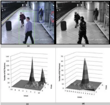
For each blob that is added to the database as a new blob, our system runs two methods, motion histogram and histogram projection [114], respectively, to estimate the number of ob-jects in the blob. Motion histogram is built by using KLT features since the magnitude and direction of KLT features of an object are mostly the same. The number of objects in the blob can be estimated by the number of peaks in the motion histogram. The motion histogram gives a correct estimation when the objects in the blob have different magnitude or direction and separates them in different bounding boxes. Each bounding box is built to include all the KLT features of a peak in the motion histogram. Figurer 3.2 (a) shows the original image with the
Figure 3.2: Motion Histogram is used to estimate the number of objects in blobs. (a) The original frame with the estimated number of objects in each blob. (b) The KLT features of comparing the frame in (a) with the previous frame. (c) The histogram of the left blob that has two objects (The man and the lady). (d) The histogram of the right blob that has one object (The man).
estimated number of objects in each blob and the corresponding KLT features are shown in Figurer 3.2 (b). Figure 3.2 (c) shows the motion histogram of the left blob that has two objects and Figure 3.2 (d) shows the motion histogram of the right blob that has one object. Clearing, in this case the motion histogram correctly estimates the number of object where the number of peaks refers to the number of objects.
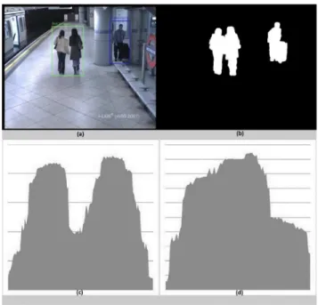
When objects are located different distances away from the camera (i.e., in the Y direc-tion), their KLT features usually have different magnitude, resulting in a correct estimation by the motion histogram. However, this may not be the case for the objects with similar Y coor-dinates. To this end, we further employ the histogram projection in the X direction for a more accurate estimation in each bounding box. The histogram projection is built by counting the foreground pixels on each point in the X direction. The number of peaks in the histogram refers to the number of objects in the blob. Figure 3.3 (a) shows the result of running the histogram
Figure 3.3:Histogram projection is used to estimate the number of objects in blobs. a) Original frame with the estimated number of objects in each blob. b) The foreground/ background of the image in (a) where two objects are in the left blob and one object is in right blob. c) The histogram of the left blob that has two objects. d) The histogram of the right blob that has one object.
projection on a frame that has two blobs. The left blob has two objects (the two ladies) and the right blob has one object (the man). Figure 3.3 (b) shows the foreground/background for the image in (a). Figures 3.3 (c) and (d) show the result of building the histogram projection for the two blobs. Clearly, in this case the histogram projection can correctly estimate the number of objects in each blob based on the number of peaks in the projection. The system repeats the examination of the blob for a number of successive frames and uses the average of the results to represent the number of objects in the blob. The system tracks the objects in the blob as one blob and tracks each object individually when it separates from the blob.
For all blobs in the database that cannot be matched in the current frame, there are two scenarios: The blob is either fully occluded or it is a stopped object. For the first case: Our system runs a Kalman filter to predict each blob’s position as we are going to explain later. The system tries to find a match between these positions and the positions of the blobs that are
added to the database as new blobs, and we update the active blob database for each match. For the second case: Our system checks the centroid of the blob in the last few frames. If there is a little change, it is considered as a stopped object and marked accordingly in the database. Finally, a blob is deleted from the database when it has no match and the prediction of the Kalman filter is out of the frame.
3.2.3
The Kalman Filter to Predict Object Position
The Kalman filter [67] is a mathematical method that uses the previous object information to predict the state of the object in the next frames. In this section, a Kalman filter is used to predict the object location after the object is full occluded or has no KLT features. Let the state vector isX = [x,y,Sx,Sy,Ax,Ay], where[x,y]is the object location,[Sx,Sy]is the object speed in thex andy directions, and [Ax,Ay]is the object area. So, the Kalman filter system model and Measurement model are:
xk =F xk−1+wk (3.5)
where: F = 1 0 1 0 0 0 0 1 0 1 0 0 0 0 1 0 1 0 0 0 0 1 0 1 0 0 0 0 1 0 0 0 0 0 0 1 (3.7) H = 1 0 0 0 0 0 0 1 0 0 0 0 (3.8)
wk :N(0,Cov1)is the process noise andvk :N(0,Cov2)is the observation noise.
3.3
Experimental Results
The proposed system can track multiple objects in real-time and efficiently deal with partial and full occlusions. Our system draws a bounding box with different color to each tracked object in the scene. A line that has the same color of the object’s bounding box is used to show the object’s trajectory. The two numbers at the top of the bounding box are used to provide the blob ID and the estimated number of objects in the blob, respectively.
We have tested the system on a computer that has AMD Sempron 2.10 GHz processor and 2.00 GB RAM. Four publicly videos are used to evaluate our proposed system. These videos consists of indoors/outdoors and one object / multiple objects testing environments.
Figure 3.4 shows an example of tracking multiple objects with partial and complete oc-clusions. The video is from the AVSS 2007 dataset. The AVSS 2007 dataset is provided by the 2007 IEEE International Conference on Advanced Video and Signal based Surveillance. Each video is digitized with a frame size 720 by 520 and rate of 25 FPS. The video includes moving persons and trains. Figure 3.4-(a) shows the foreground/background of frame 1436 in
Figure 3.4: Tracking multiple objects with occlusion handling. (a) The foreground/background image of frame 1436 shows the occlusion. (b) The result of our tracking system of frame 1436. (c) The foreground background image of frame 4484 shows the occlusion. (b) The result of our tracking system of frame 4484.
Figure 3.5: The result of our tracking system for multiple objects in frames 1337, 1347, 1357, 1367, 1377, and 1387 of AVSS 2007 video. The original frames have the tracking results and foreground background images show the partial occlusion of one car by another.
Figure 3.6:The result of our tracking system for multiple cars.
Figure 3.4-(b), and three objects are merged together. Cleary, our system tracks the two per-sons after they disappear behind the pole (full occlusion) and show up again. In addition, the three objects -the two guys and the lady- are tracked during the partial occlusion as shown in Figure 3.4-(b). Figure 3.4-(c) shows the foreground/background of frame 4484 from the same video sequences and the two guys are merged in one blob. Each object of the three objects in the frame 4484 is tracked individually without any effect to partial occlusion as shown in Figure 3.4-(d). So, a correct segmentation is made during the partial occlusion and each object is tracked individually.
Figure 3.5 shows an example of tracking multiple objects during partial occlusion. The video is from the AVSS 2007 dataset. The video includes moving persons and cars. Figure 3.5 shows the result of tracking multiple cars where one car is partially occluded by another one for about 50 frames as the foreground background images show. Our system smoothly and nicely tracks the multiple objects with and without occlusion.
Figure 3.6 shows the result of tracking multiple objects in video sequences that are selected from are real surveillance videos that are taken on intersections during daytime. The moving cars are tracked nicely as shown by the different colors for the bounding boxes and trajectories as Figures 3.6 (a) and (c) show. For a more complex scene, Figure 3.6-(b) shows multiple stop-and-go cars, in which some cars stop for a short time before the traffic light and then start
Figure 3.7:The result of tracking an object by using Predator (first row) and our system (second row).
moving again. Our system keeps tracking them and maintains a bounding box around each car. We also compared our system with a state-of-the-art tracking system that is called Predator [64] as Figure 3.7 shows. The first row in Figure 3.7 shows the results of using Predator to track an object in a subway and the second row shows the results of tracking the same object by using our system. The object is tracked nicely in our system where Predator failed.
3.4
Summary
In this chapter, we have proposed a novel tracking system for effectively tracking objects in surveillance videos. The proposed system is composed of two components: An improved KLT tracker, and a Kalman filter. The improved KLT tracker uses the basic KLT tracker and an appearance model to track objects from one frame to another and deal with partial occlusion. In partial occlusion, the appearance model (e.g., a RGB color histogram) is used to determine an object’s KLT features during partial occlusion, and we use these features for accurate and robust tracking. In full occlusion, a Kalman filter is used to predict the object’s new loca-tion and connect the trajectory parts. The experimental results demonstrated that our system successfully tracks multiple objects with partial or full occlusions.
CHAPTER 4
SEGTRACK: A NOVEL TRACKING SYSTEM WITH
IMPROVED OBJECT SEGMENTATION
4.1
Introduction
Most tracking methods depend on a rectangle or an ellipse mask to segment and track objects. Typically, using a larger or smaller mask than the actual object will lead to loss of tracked objects. In this section, we propose SegTrack [11] : an object tracking system that is more efficient in dealing with partial and full occlusion as shown in Fig. 4.1. Our improved mixture of Gaussians segments foreground objects from the background and solves stop-then-move and stop-then-move-then-stop problems. Then, KLT tracker tracks objects in consecutive frames and detects partial and full occlusions. In partial occlusion, a novel silhouette segmentation al-gorithm evolves the silhouettes of occluded objects by matching the location and appearance of occluded objects between successive frames. In full occlusion, one or more feature vectors for each tracked object are used to re-identify the object after reappearing. SegTrack is evaluated by comparing it with other state-of-the-art methods on public video datasets. The rest of this chapter is organized as follows: Section 4.2 describes the SegTrack system, and Section 4.3 presents the experimental results on different testing videos. Finally, Section 4.4 summarizes.
4.2
SegTrack
4.2.1
Background Subtraction.
The first step in SegTrack is segment the foreground object from the background by apply-ing background subtraction [134] as explain in 3.2.1. In SegTrack, the statistical background model is built by using a mixture of Gaussians [63]. The output of the background subtrac-tion module is a set of foreground blobs where each blob consists of one or more (overlapped) objects.
Figure 4.1: Results from SegTrack. The first column shows a person stops for a long time and remains as a foreground object. The second column shows a person starts moving after he stops for a while, and the ghost foreground is detected and deleted. The third column shows tracking results with simple and severe partial occlusions. The fourth column shows the tracking results with full occlusion.
Adapting the mixture of Gaussians at a slower rate than the foreground scene produces false foreground areas (ghosts) [110], a problem referred as the ”stop-then-move” problem. SegTrack determines if a blob is a ghost based on the ratio between the ghost pixels and the border pixels, where a border pixel is a contour pixel whose eight neighborhood contains non-foreground pixels, and a ghost pixel is a border pixel and does not belong to any neighborhood Gaussian models. If the ratio is bigger than a threshold, the blob is deleted from the foreground. The second problem is move-then-stop problem where stopped object may become as a part of the background model after a few frames. SegTrack deals with the problem by preventing the blob regional pixels from participating in the background updates if there is no change to the blob location (stopped blob).
4.2.2
KLT Tracker.
The foreground blobs are tracked from one frame to another by using the improved KLT tracker as explain in Section 3.2.2. After removing inaccurate KLT featuers, SegTrack uses the remaining KLT features to connect between blobs in consecutive frames. KLT tracker detects the partial occlusion if a new blob in the current frame is matched to more than one blob in the previous frame. In this case, a silhouette-based segmentation method is used to evolve
each object’s silhouette in the occluded region. Then, the KLT features are used to match the evolved blobs with the previous existing blobs. All old blobs that cannot be matched in the current frame are considered as fully occluded blobs.
4.2.3
Silhouette Segmentation Algorithm
Many tracking systems use probabilistic model to segment objects during occlusions. Pre-vious knowledge and learning are main concerns as no information in real time video about tracked objects is known until they appear at the first time. In addition, some of these systems evaluate all foreground pixels with the probabilistic model without using the object’s previous location, which is critical in tracking. Our silhouette segmentation algorithm uses the objects locations in previous frame to improve the segmentation results and reduce the number of eval-uated foreground pixels. The silhouette segmentation algorithm is run only when the merged blobs (partial occlusion) are detected as we explained in the previous section. The silhouette for each object is evolved as follows:
First: The Teh-Chin chain approximation algorithm is used to evolve the contour of each
blob (B) in the previous frame (Fi = {Bi1, Bi2, ..., Bin}). The algorithm determines the sup-port region of a point (pi) as follows [120]:
D(pi) = {pi−k, ..., pi−1, pi, pi+1, ..., pi+k} (4.1)
The length of the support region (k) starts with k=1 and keeps increasing by one until inequality (4) or both inequalities in (5) hold:
or dik lik ≥ di,k+1 li,k+1 for dik >0 (4.3) dik lik ≤ di,k+1 li,k+1 for dik <0
where the length of the chord joining the pointspi−kandpi+k islik =|pi−kpi+k|, and(dik)is the perpendicular distance of the pointpito the chordpi−kpi+k. Each point should survive from the following operations, whereSis the measure of significance andCU Ris the curvature (see [120] for more details):
|S(pi)| ≥ |S(pj)| for allj: |i−j| ≤ki/2 (4.4)
CU Ri1 = 0
if([kiofD(pi)] = 1)and(pi−lorpi+lstill survived)then
if(|S(pi)| ≤ |S(pi−l)|)or(|S(pi)| ≤ |S(pi+l)|)then further suppress pi
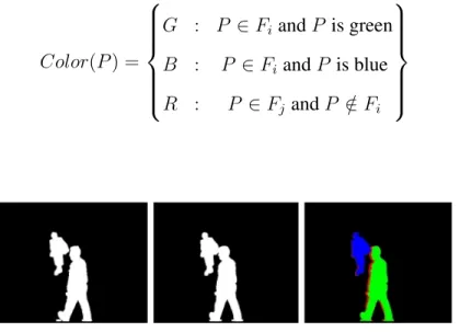
Second: One contour from the list of contours that are computed in first step is chosen as
our target contour. A green color (G) is given to the target contour pixels (P) and a blue color (B) is given to all other contour’s pixels as follows:
Color(P) = G : P ∈Bik. B : P ∈Bitandk 6=t. (4.5)
Third: Match the result from step two with the current foreground image (Fj) and color
(4.6). Fig. 4.2 shows the result of matching two consecutive foreground images. Color(P) = G : P ∈Fi andP is green B : P ∈FiandP is blue R : P ∈Fj andP /∈Fi (4.6)
Figure 4.2: Result of comparing two consecutive frames.
Fourth: For each red pixel (Pr), it is used as a centroid of a rectangle (Rct) whose size
is determined by the maximum moving speed of the tracked objects in this blob. The green (Pg) and blue (Pb) pixels in the previous frame, before objects merging, are used as a base of comparing as we know which pixel belongs to which object exactly. The comparison is done using the nearest neighbor algorithm by computing the Euclidean distance (ED) in theRGB
color space. The red pixels are the recolored as follows:
∀Pg ∈Rct and ∀Pb ∈Rct (4.7)
Find ED(RGB(Pr∈Fj), RGB(Pg ∈Fi))
Find ED(RGB(Pr∈Fj), RGB(Pb ∈Fi))
Keep the Nearst NeighborP(PN N)
Color(Pr) = G : PN N is Green B : PN N is Blue
distance to other objects is larger than the target object’s speed. This is important to maintain a sufficient space between tracked objects to obtain accurate contours for the next iteration. Then open morphology is run to smooth the contour for current object (green pixels). The new foreground image is used as a base of matching with the next frame if occlusion is detected. Otherwise, the foreground image from background subtraction will be used. Finally, if the size of an object becomes very small due to heavy occlusion, for example, less than 10% of its original size before occlusion, SegTrack treats it as a full occluded object.
4.2.4
Person Re-identification.
Object re-identification solves full occlusion cases that are detected in the KLT tracker as explained in section 4.2.2. We cast the object re-identification problem into a distance problem. For blob (A) that is marked as a full occluded blob in the database, we need to successfully identify the blob if it is recaptured elsewhere in space and time. This can be achieved by using a distance functionD(B1, B2)so that:
D(B1, B2)< threshold (4.8)
where B1 and B2 are different blobs for the same target blob (A). Due to computing time
concerns, we use a fast distance matching method, i.e., the Bhattacharyya distance [47] defined in Equation (4.9), D(V1, V2) = s 1− p 1 ¯ V1V¯2N2 X p V1.V2 (4.9)
whereV1 andV2 are the feature vectors forB1 andB2, respectively, andN is the vector length
The feature vector for each target is built by dividing the target image into three horizontal strips: head, upper body and lower body with (1:2:3) as the ratio. Because the head does not have many distinctive features, it is not used. For the upper and lower body, the RGB and HSV are computed and represented as histograms. Each channel is represented by a16dimensional
histogram vector, and thus each target image is represented by a192dimensional feature vector. The RGB and HSV are common color spaces to represent a object’s appearance [140]. However, viewing condition, occlusion, and illumination and pose changes will cause signif-icant appearance variations. Finding distinctive and stable features are extremely hard if not impossible. To deal with this issue, more than one feature vector are built for each tracked blob. The first feature vector is obtained when a blob is added to the database as a new blob. Another feature vector is added for the same blob during tracking when the matching distance between the current feature vector and all other feature vectors of the same blob is higher than a threshold.
4.3
Experimental Results
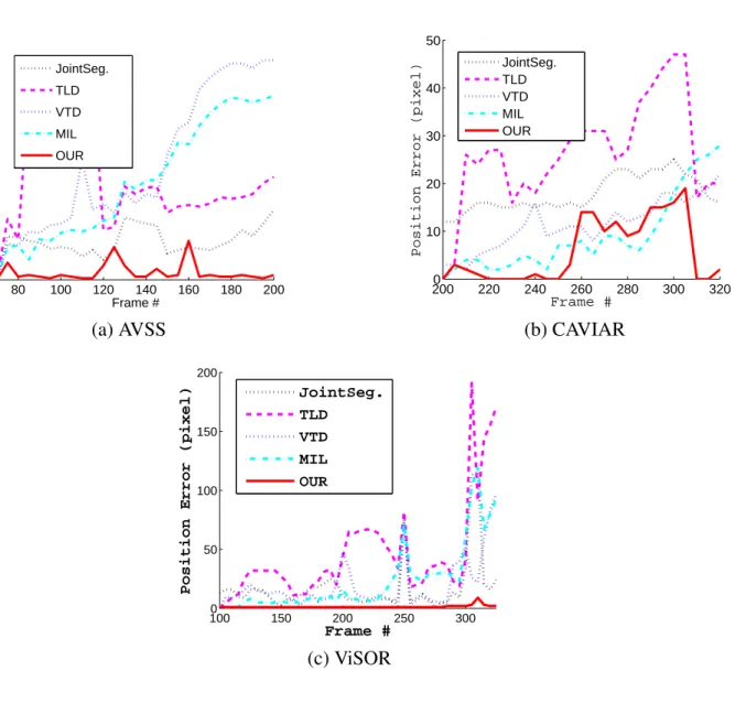
We tested SegTrack on several challenging video sequences from PETS 2006 [3], CAVIAR [1], AVSS 2007 [4] and ViSOR [5] datasets. We compare SegTrack results with several state-of-the-art tracking methods, i.e., TLD [64], Joint Seg. [7], MIL [16] and VTD [71]. Specifi-cally, TLD uses positive and negative samples that are collected during tracking to build and improve the performance of a detector. KLT features are used to track the object. The detector is employed to find the object if the tracker fails. Joint Seg. uses a probabilistic framework based on background subtraction and pixel-level segmentation method to track objects. The MIL method builds and updates a detector with a set of the object images even though the image is not precisely for the object. The VTD method uses multiple observation and motion models, each of which covers a different type of observation or motion. Then, the results are integrated into one tracking system.
SegTrack is implemented using OpenCV and C++ language on a machine that has a Quad (2.83GHz and 3.01GHz) processor and 4GB RAM. The codes for TLD, Joint Seg., MIL and VTL are obtained from the authors with default parameter setting. For all the video sequences that are used in our experiments, we manually labeled the ground truth center of each object every 5 frames. The average center location error is used as a comparison base. The average
80 100 120 140 160 180 200 0 50 100 150 Frame #
Position Error (pixel)
JointSeg. TLD VTD MIL OUR (a) AVSS 2000 220 240 260 280 300 320 10 20 30 40 50 Frame #
Position Error (pixel)
JointSeg. TLD VTD MIL OUR (b) CAVIAR 1000 150 200 250 300 50 100 150 200 Frame #
Position Error (pixel)
JointSeg. TLD VTD MIL OUR (c) ViSOR
Figure 4.3: Error plots for three video clips.
center error was computed only for the frames in which a method was able to track all targets. The quantitative results are summarized in Table4.1 and Fig.4.3.
4.3.1
Background Subtraction
The background subtraction, the first step in SegTrack, is used to segment foreground ob-jects with an average frame rate of42frame per second. Fig. 4.4 shows results of our improved mixture of Gaussians method, where the move-then-stop and stop-then-move problems are solved. The first row shows the original four frames from the PETS 2006 dataset where a