Learning to Map the Visual and Auditory World

(1)

University of Kentucky University of Kentucky

UKnowledge

Theses and Dissertations--Computer Science Computer Science

2019

Learning to Map the Visual and Auditory World

Tawfiq Salem

University of Kentucky, [email protected] Author ORCID Identifier:

https://orcid.org/0000-0001-6232-0542

Digital Object Identifier: https://doi.org/10.13023/etd.2019.340

Right click to open a feedback form in a new tab to let us know how this document benefits you. Right click to open a feedback form in a new tab to let us know how this document benefits you.

Recommended Citation Recommended Citation

Salem, Tawfiq, "Learning to Map the Visual and Auditory World" (2019). Theses and Dissertations--Computer Science. 86.

https://uknowledge.uky.edu/cs_etds/86

This Doctoral Dissertation is brought to you for free and open access by the Computer Science at UKnowledge. It has been accepted for inclusion in Theses and Dissertations--Computer Science by an authorized administrator of UKnowledge. For more information, please contact [email protected].

(2)

STUDENT AGREEMENT: STUDENT AGREEMENT:

I represent that my thesis or dissertation and abstract are my original work. Proper attribution has been given to all outside sources. I understand that I am solely responsible for obtaining any needed copyright permissions. I have obtained needed written permission statement(s) from the owner(s) of each third-party copyrighted matter to be included in my work, allowing electronic distribution (if such use is not permitted by the fair use doctrine) which will be submitted to UKnowledge as Additional File.

I hereby grant to The University of Kentucky and its agents the irrevocable, non-exclusive, and royalty-free license to archive and make accessible my work in whole or in part in all forms of media, now or hereafter known. I agree that the document mentioned above may be made available immediately for worldwide access unless an embargo applies.

I retain all other ownership rights to the copyright of my work. I also retain the right to use in future works (such as articles or books) all or part of my work. I understand that I am free to register the copyright to my work.

REVIEW, APPROVAL AND ACCEPTANCE REVIEW, APPROVAL AND ACCEPTANCE

The document mentioned above has been reviewed and accepted by the student’s advisor, on behalf of the advisory committee, and by the Director of Graduate Studies (DGS), on behalf of the program; we verify that this is the final, approved version of the student’s thesis including all changes required by the advisory committee. The undersigned agree to abide by the statements above.

Tawfiq Salem, Student Dr. Nathan Jacobs, Major Professor Dr. Miroslaw Truszczynski, Director of Graduate Studies

(3)

Learning to Map the Visual and Auditory World

DISSERTATION

A dissertation submitted in partial fulfillment of the requirements for the degree of Doctor of Philosophy in the

College of Engineering at the University of Kentucky

By Tawfiq Salem Lexington, Kentucky

Director: Dr. Nathan Jacobs Associate Professor of Computer Science

Lexington, Kentucky 2019

(4)

ABSTRACT OF DISSERTATION

The appearance of the world varies dramatically not only from place to place but also from hour to hour and month to month. Billions of images that capture this complex re-lationship are uploaded to social-media websites every day and often are associated with precise time and location metadata. This rich source of data can be beneficial to improve our understanding of the globe. In this work, we propose a general framework that uses these publicly available images for constructing dense maps of different ground-level at-tributes from overhead imagery. In particular, we use well-defined probabilistic models and a weakly-supervised, multi-task training strategy to provide an estimate of the ex-pected visual and auditory ground-level attributes consisting of the type of scenes, objects, and sounds a person can experience at a location. Through a large-scale evaluation on real data, we show that our learned models can be used for applications including mapping, image localization, image retrieval, and metadata verification.

KEYWORDS: computer vision, machine learning, deep neural networks, remote sensing, geospatial analysis, mapping

Author’s signature: Tawfiq Salem

(5)

By Tawfiq Salem

Director of Dissertation: Nathan Jacobs

Director of Graduate Studies: Miroslaw Truszczynski

(6)

This work is dedicated to the memory of my parents, Mousa and Huda Salem. I would have never become who I am now without their inspiration and limitless love and support.

They taught me the importance of commitment, hard work, and going above and beyond to achieve my goals and dreams.

(7)

ACKNOWLEDGMENTS

I would like to express my sincere appreciation and gratitude to my advisor, Dr. Nathan Jacobs, for his constant encouragement, support, and guidance throughout my doctoral program. Dr. Jacobs was always there to listen to me and to give me sincere advice. He showed me different ways to approach a research problem. More importantly, he inspired me to work hard by being a role model himself. I would have never completed my research work without his help, guidance, and support.

My sincere thanks go to the rest of my committee members, Dr. Seales, Dr. Yang, and Dr. Cheung for their helpful feedback and discussions which helped me curate this docu-ment and present my work in a meaningful way. Special thanks to Dr. Sama for agreeing to be my outside examiner in my defense. I am grateful to the graduate coordinator, Dr. Mirek Truszczynski, for his encouragement and support during my Ph.D. studies. I would also like to extend my thanks to all the faculty members of the computer science department for providing me with a solid foundation, not only in computer science but also in academia.

I will forever be thankful to my lab-mates, including Scott Workman, Menghua Zhai, Zach Bessinger, Connor Greenwell, Weilian Song, M. Usman Rafique, Hunter Blanton, and others. We have all been there for one another and have taught ourselves and each other many tools and skills. I know that I could always ask them for advice, opinions, and ideas on different research problems. Thank you all for the fun and support. I am eagerly looking forward to having all of you as colleagues in the years ahead.

Last but not least, I would like to thank my family, whose continuous love, support, and encouragement have been the light of my life. My brothers and sisters, thank you for your support, and special thanks goes to my brother, Saeed Salem, who was the first person to encourage me to pursue a graduate education. And, of course, thanks for the constant support through the ups and downs of my academic career. To my son Bilal and my daughters Jena and Huda, you have always been a source of joy, inspiration, and encouragement to work hard toward achieving my goals. To my wife, Wafaa, who inspired me all the time and for the endless love and support she provided during my journey.

(8)

3.3 Visual appearance changes dramatically due to differences in location and time. Our work takes advantage of sparsely distributed, ground-level image data, with associated location and time metadata, in conjunction with overhead im-agery to construct dynamic maps of visual appearance attributes. . . 14

4.1 An overview of our network architecture. . . 18

4.2 For a given ground image, we show the top-3 overhead images that give the highest probability for the given image. The top row is based on Places, the second on Imagenet, and the last on Object counts. . . 20

4.3 Given a query ground-level image (left), we can construct a heatmap (right) that represents the score where the greener the dot on the map the more likely the image was taken in that location. . . 21

4.4 Localization accuracy of the different learned probabilistic models on the test-set of the ground-level imagery . . . 22

4.5 Overhead images with the highest scores for thecarlabel. Theparklabel score is increased from left to right, transitioning the images from industrial to rural scenes while focusing on roads. Each column represents multiple images with similar scores for the query labels. . . 22

(11)

5.1 Visual appearance changes dramatically due to differences in location and time. Our work takes advantage of sparsely distributed, ground-level image data, with associated location and time metadata, in conjunction with overhead im-agery to construct dynamic maps of visual appearance attributes. . . 25 5.2 An overview of our network architecture, which includes the network we train

to predict visual attributes (left) and the networks we use to estimate visual attributes (right). . . 27 5.3 The spatial distribution of the dataset. The green (red) dots represent the

train-ing (testtrain-ing) data. . . 30 5.4 The temporal distribution of the dataset. . . 31 5.5 Dynamic visual attribute maps for different transient attributes and months. In

each, yellow (blue) corresponds to a higher (lower) value for the corresponding attribute. Each attribute exhibits unique spatial and temporal patterns, which closely match the authors’ personal travel experiences. . . 33 5.6 Dynamic visual attribute maps for different methods on the transient attribute

sunny. . . 33 5.7 For a given location and corresponding overhead image, predictions of the

sunrise-sunsetattribute at different hours for two different months. This high-lights that our model has learned that days are longer during the summer. . . 35 5.8 For each overhead image, we predict the visual attributes using our full model

and compute the average distance between them and those of the ground-level images in the test set. (left) The overhead images of two query locations. The closest images when using August at 5pm as input (middle) and when using August at 2am (right). . . 35 5.9 Localization accuracy as a function of candidate images searched. Our

ap-proach,image+time+loc, outperforms all baselines. . . 36 5.10 Given a query ground-level image (top), we show localization results (bottom)

for different scoring strategies, visualized as a heatmap. Red (blue) represents a higher (lower) likelihood that the image was captured at that location. . . 37

(12)

5.11 An example highlighting temporal patterns learned by our model. For each example, we show the original image and the overhead image of its location. For every possible hour and month, we use our full model to predict the visual attribute. The heatmap shows the distance between the true and predicted vi-sual attributes, with dark green (white) representing smaller (larger) distances. In the top example, there are two narrow bands of small distances, centered around dawn and dusk. In the top example, we see small distances during the

nighttime hours. . . 38

6.1 We propose a multimodal approach for relating overhead image appearance with sounds in order to map soundscapes. (left) Overhead image; (right) Simi-lar ground-level images and sounds output by our method. . . 42

6.2 An overview of our network architecture. . . 43

6.3 The distribution of the collected audio files in our CVS dataset. . . 44

6.4 A word cloud for the tags associated with the sounds in the CVS dataset. . . 45

6.5 The model architecture for predicting a distribution over sound clusters from an overhead image. . . 46

6.6 Our work explores the relationship between overhead image appearance and sound. Given an overhead image (top), our model outputs a distribution over sound clusters (bottom). . . 48

6.7 Block-level audio mapping: (left) An overhead image of a small geographical region on Miami beach. (right) A per-pixel labeling of sound clusters. . . 48

6.8 City-level audio mapping: (left) An overhead image covering New York City. (right) A per-pixel labeling of sound clusters. . . 48

6.9 Country-level audio mapping: visualizing the sound clusters over USA. Gaps (white) are regions where the CVUSA dataset does not have imagery. . . 49

(13)

LIST OF TABLES

5.1 Comparing performance on the visual attribute prediction task. . . 32

(14)

Chapter 1 Introduction

“Even before you understand them, your brain is drawn to maps.”

– Ken Jennings

Looking at the world from above, you will see a diverse range of scenery, from mountains to beaches, deserts to rainforests, and many other types of scenery. Furthermore, the ap-pearance of the same scene may change over time. For example, if we were to look at a forest in summer, we will expect to see green trees and sunny weather, whereas if we look at it in winter, we will likely see leafless trees and snowy weather. Depending on geoloca-tion and time, our world can look very different. One of the most efficient ways to represent these differences is by maps. Maps can represent our big world at a much smaller scale for people to explore and provide information that helps them decide where to live and how to travel from a location to another. Moreover, cities and countries often use maps for monitoring land-use and land-cover changes, especially those caused by human activities, and help them in making decisions toward planning and development.

There are many different types of maps based on the information they provide. For example, a street map shows you roads, their names, and different points of interests along these roads. A topographic map represents information about land elevations and features, a park map that shows you trails and playgrounds, and a city map shows the roads and locations of important buildings such as hospitals. Constructing such maps at a global scale can be very costly and time-consuming since there will be a need to collect information from all over the world.

Recently, the widespread use of social media and the increasing availability of smart-phones have conveniently allowed people to capture and share most of their life activities in terms of images and videos. This data is often associated with precise time and loca-tion metadata. Moreover, advances in remote sensing and satellite technologies enabled

(15)

Figure 1.1: The semantic content of the overhead image and the co-located ground level image are similar.

the accumulation of overhead imagery that covers most of the globe. Currently, billions of geotagged images are publicly available on the Internet. This rich source of images, com-ing from all over the world, could be very beneficial to better understand our globe. This dissertation proposes a general framework for utilizing these publicly available images for mapping different ground level attributes.

1.1 Image Driven Mapping

When we, as humans, look at an image it does not take much effort for us to recognize a cat or a human face in the image. Although humans perform these tasks effortlessly, these are actually hard problems to solve with a computer since computers see an image as a

(16)

matrix of numbers. In computer vision, researchers focus on how computers can learn to gain high-level understanding from digital images or videos. Different works in computer vision have focused on different ground-level image understanding tasks, such as image classification [26, 56] and object recognition [60, 74]. Researchers have also proposed algorithms for estimating image attributes including scene classification [64, 80], weather estimation [7, 33], and image geolocalization [25, 68].

Recently, with the availability of large datasets of geotagged images, different works have proposed methods for mapping ground-level attributes based on ground-level image appearance. Gebru et al. [19] proposed a method for estimating and mapping socioeco-nomic characteristics of different US cities using millions of Google street-view images. Another work by Arietta et al. [4] proposed a method for automatically identifying and mapping the relationships between the visual appearance of a city and its non-visual at-tributes including crime statistics, housing prices, and population density. Other proposed methods for mapping people’s visual appearance [10, 28]. Because of the sparsity of the existing ground-level imagery, methods proposed to map ground-level attributes based on ground-level images lack the ability to generate dense maps at a global scale. Furthermore, these methods are biased towards locations with large numbers of ground-level images.

1.2 Mapping Using Overhead Imagery

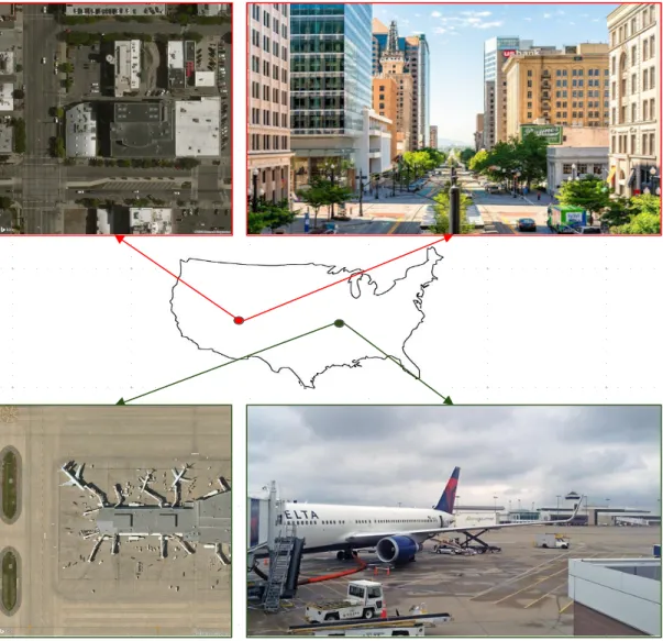
To tackle the problem of sparsely distributed ground-level imagery, this dissertation pro-poses a general framework for mapping ground-level attributes from overhead imagery. Although overhead imagery is uniformly distributed and available for almost every loca-tion on earth, the lack of annotated data for model training remains a challenge for learning from overhead imagery. However, pairing overhead and co-located ground images gives hope at tackling this challenge. If we were to look at the different pairs of overhead and the co-located ground-level images in Figure 1.1, we will notice the similarity in the semantic contents of the different views. The overhead image (left) in the top row shows an image covering a city with roads and buildings, and we can see similar content if one looks at the ground image (right) taken at the center of the overhead image. We can also notice the same observations in the bottom pair of images that cover an airport with runways, terminals, and airplanes.

Several existing works have approached this problem. For example, Lee et al. [35] proposed an approach to estimate geo-informative attributes such as population density and demographic properties. Similar to our approach, the work in [70] proposed a method for mapping between ground-level and overhead image and utilized the proposed method

(17)

for the problem of image localization. The previous methods assumed that the predictions of the ground-level images were distributed in a Gaussian manner, and only learned to predict the mean of the distribution. This is problematic when a particular overhead image could have multiple possible scenes. For example, the overhead image (left) in the top row in Figure 1.1 covering parks, stadium, and parking lots.

To capture this multi-label feature of images, we propose to learn probabilistic models that capture the distribution of the different ground-level image labels. We also introduce a method for constructing dynamic maps at a global scale, which is a probability distribution conditioned not only on the geographic location but also on time. These maps capture the change in different ground level attributes over time. To the best of our knowledge, our work is the first to integrate dense overhead imagery with location and time metadata to better model the relation between image appearance, location, and time. We further propose a method for mapping soundscapes to show the type of sounds one can hear at a given geolocation.

1.3 Contributions

In this work, we propose a general framework for mapping ground-level attributes from overhead imagery. We propose different models for constructing static and dynamic maps for different types of attributes. We also conduct different experiments to show the different applications of our proposed methods. For the purpose of the research in this dissertation, a map can be thought of as a probability distribution, conditioned on geographic location, over a collection of attributes; typical attributes include land cover, land use, elevation, or place name.

Main Contributions: The main contributions of this dissertation are:

• A general framework based on deep convolutions neural networks for mapping ground-level attributes.

• A model for constructing a static map that captures the change in the type of scenes, objects, and object counts from overhead imagery.

• A model for constructing dynamic maps for different ground-level attributes that change over time and geolocation.

• A model for understanding the types of sounds that could be heard at a specific geographic location and mapping the soundscapes at a global scale.

• A detailed evaluation, both quantitative and qualitative, of the learned models for a variety of different settings.

(18)

• Present different applications for these models, including mapping, image localiza-tion, image retrieval, and metadata verification.

1.4 Dissertation Outline

The remainder of this document consists of the following chapters:

• Chapter 2provides a technical background that is necessary for understanding the work in this dissertation. We provide an overview of related research works in three areas: learning with convolutional neural networks, transfer learning, and image at-tributes.

• Chapter 3 presents a general framework for mapping ground-level attributes from overhead imagery. A key element of our approach is that we use visual attributes present in ground-level images as a supervisory signal for model training, thus re-quiring no labeled overhead imagery.

• Chapter 4 introduces an approach that makes it possible to draw a variety of con-clusions from overhead imagery. In particular, we propose using well-defined proba-bilistic models and a weakly-supervised, multi-task training strategy to learn to pre-dict properties and their uncertainties for a given location. We show that our learned models can be used directly for applications in mapping and image localization. The material in this chapter has been published [50].

• Chapter 5introduces an approach for constructing dynamic maps of visual appear-ance attributes that can provide an estimate of the expected appearappear-ance at any ge-ographic location and time. Our approach integrates dense overhead imagery with location and time metadata. A key element of our method is that we use visual at-tributes present in ground-level images as a supervisory signal for model training, thus requiring no labeled overhead imagery. Through a large-scale evaluation on real data, we find that combining overhead imagery with metadata results in more accurate predictions and better performance on a variety of tasks.

• Chapter 6 explores the problem of mapping soundscapes, that is, predicting the types of sounds that are likely to be heard at a given geographic location. Using a novel dataset, which includes geo-tagged audio and overhead imagery, we develop an approach for constructing an aural atlas, which captures the geospatial distribution of soundscapes. We build on previous work relating sound to ground-level imagery

(19)

but incorporate overhead imagery to overcome the limitations of sparsely distributed geo-tagged audio. In the end, all that we require to construct an aural atlas is over-head imagery of the region of interest. We show examples of aural atlases at multiple spatial scales, from block-level to country. The material in this chapter has been pub-lished [52].

• Chapter 7summarizes the contributions of this dissertation and our most important findings. In addition, we discuss possible future research directions that will lead to improved methods for geo-visual analysis and understanding.

(20)

Chapter 2 Technical Background

In this chapter, we provide an overview of related research works in two areas: learning with convolutional neural networks and present the different techniques for transfer learn-ing.

2.1 Learning with Convolutional Neural Networks

A neural network is a computational model that is inspired by the way biological neural networks in the human brain process information. Convolutional Neural Networks (Con-vNets or CNNs) is a category of neural networks that has gained attention since Alex Krizhevsky [32] developed the AlexNet structure and used it in 2012 to win the ImageNet competition (classifying 1.2 million images to 1.000×103 classes). AlexNet consider-ably outperformed the previous state-of-the-art methods, dropping the classification error from 26% to 15%. Since then CNNs has generated a lot of excitement in research and industry. Researchers in computer vision continue using CNNs and have shown great suc-cess on traditional computer vision problems: image classification [26, 56], object recog-nition [60, 74], and scene classification [64, 80]. Furthermore, different big companies

(21)

started employing deep learning in their services, such as face recognition at Facebook, photo search at Google, product recommendation system at Amazon. One of the main reasons behind the great performance of CNNs is its ability to learn hierarchical features representation of the input images while traditional methods use hand-engineered features. How CNNs learns the hierarchical features representation of an image? computers see an image as an array of numbers with size equals width×height×channels. For example, in image classification the input is an image, array of numbers, and the expected output is a probability distribution over the different classes that the input image belongs to. To perform image classification, CNNs looks for low-level features such as edges and curves in the training images and then construct abstract concepts through a series of linear and nonlinear operations achieved by a combination of layers.

The major components of a CNNs model is a number of convolutional and subsam-pling layers optionally followed by fully connected layers. The excellent performance of CNNs most of the time come on problems that involve learning discriminative models that usually map a high-dimensional data (e.g. image) to a class label as shown in Figure 2.1. This learning approach, known as supervised learning, for training convolutional neural networks depend on large amounts of labeled samples (training data). Different problems lack the amount of labeled data required for training CNNs. The common practice in deep learning for such problems is to use transfer learning approaches.

2.2 Transfer Learning

The traditional method for training CNNs on a discriminative problem depends on the availability of labeled data. For example, the performance improvement achieved in Krizhevsky et al. [32] was only possible due to the existence of massive training labeled records (1.2 Million training-set). Nowadays, researchers rarely train an entire CNNs model from scratch (with random initialization), because it is hard and costly to have enough training labeled data [76]. Instead, it is a common practice to use and adapt pre-trained models for the new related task of interest. Next, we will explain in more details the different ways to use pre-trained models on a new related task.

2.2.1 Fixed feature extractor

Different works have shown that the features extracted from a model trained on a task can be useful for other related tasks. Razavian et al. [55] have shown that features extracted from OverFeat [54] that has the same structure as AlexNet and trained on ImageNet,

(22)

per-Figure 2.2: The common way of extracting features from a model is by removing the last couple of layers and use the rest of the model to extract features for input data from the new task.

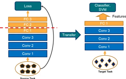
formed reasonably well on a whole variety of tasks, including image classification, and image retrieval. A common way of extracting useful features from a well-trained model such as pre-trained AlexNet is by removing the last fully-connected layer(s) and using the rest of the trained-model as a fixed feature extractor for the new data on the new domain. Different classifiers, e.g. SVM, can be applied over the extracted features as shown in Fig-ure 2.2. A recent work by Owens et al. [45] proposed a method for learning scenes and object detection by training a model for predicting the audio label from an image. Then, extracted the mid-level features from this model for thousands of images and found that different neurons are selective on specific objects and showed that these mid-level features can be very helpful for object and scene detection and classification.

2.2.2 Domain Adaptation

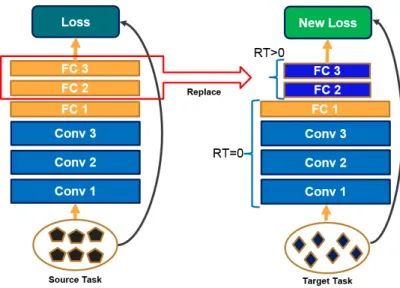
Would it be possible to do better than off-the-shelf features? the answer is yes in many of the cases by what is known as domain adaption. In domain adaptation, we start with a well-trained model for a ‘nearby’ task, such as AlexNet that has been trained on 1.2 million images for image classification, and you cut off the top layer(s) and replace it with a new layer(s) suitable for the new related task. We fine-tune the new network by running iterations of stochastic gradient descent and back-propagation on the training data for the new problem with new loss function as can be seen in Figure 2.3. It is possible to fine-tune all the layers of the new model or keep some of the earlier layers fixed and only fine-tune some higher-level portions of the network.

(23)

Figure 2.3: The general approach for fine-tuning a pre-trained model on a new related problem.

Figure 2.4: The general approach for model-to-model learning.

This is motivated by the observation that the earlier features of convolutional networks contain lower level features, e.g. edges and curves that should be useful to many differ-ent tasks, but the final layers of the convolutional networks learn high-level details of the classes contained in the original dataset. This approach usually results in faster training times than training new convolutional networks from scratch [16, 18, 22, 63].

(24)

2.2.3 Knowledge Distillation

Over the past few years, deep learning techniques have enabled rapid progress on different core problems in computer vision including, image classification and detection. One of the main challenges in training an efficient deep learning model on a new problem is the need for lots of data which is most of the time hard and costly to obtain. Recently, Ba et al. [6] proposed a training procedure to transfer knowledge from a previously trained model (teacher) that achieve high performance to a model on a related task (student) as shown in Figure 2.4. Different work recently used this approach, e.g., the work by Work-man [70] proposed a cross-view training approach for learning to predict the scenes cat-egories from overhead-imagery. Workman et al. [70] used the prediction of the last layer of the well-trained AlexNet-Places model that produces a categorical-distribution over250 scenes categories for any given outdoor ground-level image as a weak signal during train-ing. Another interesting work by Aytar et al. [5] proposed a method for transferring from vision to other modalities and built a model of learning sound features using two vision-based trained models, Places-CNN and ImageNet-CNN. Similar to this, in this work we use models trained on the ground-level to provide a supervisory signal to train models on co-located overhead imagery.

(25)

Chapter 3 General Framework for Mapping

Geospatial Attributes

This dissertation proposes a general framework that exploits the publicly available data and the similarity between overhead and ground imagery to make it possible to draw wide-ranging conclusions from overhead imagery. In particular, we propose leveraging the recent advances in ground-level image understanding to learn and map different ground-level attributes from overhead-imagery without requiring annotated data. The proposed approaches utilize pre-existing CNNs to extract categorical distributions of co-located ground-level images to provide a weak signal for training models on overhead imagery. The unique advantages of our proposed methods are: 1) it can operate at a global scale and 2) they are not prone to the bias of sparse data since overhead imagery is uniformly distributed and available for almost every location on earth.

3.1 Estimating Images Attributes

The word attribute is a generic term and it can refer to any property that is associated with the image’s appearance. It takes us, Humans, a single glance to make a higher-level judgment about a scene as a whole; whether it is a park, airport, or Museum as shown in Figure 3.1b. Different works in computer vision have focused on the problem of scene recognition. The work by Zhou et al. [80] proposed a model calledPlaces-CNNusing a neural network that has been trained on over two million images from 205 places cate-gories, and then the same authors proposed a new model calledPlaces2trained on over ten million images from 365 places categories. Other works have been proposed for estimating the age and gender based on the human appearance in an image [37, 75], the date of when

(26)

(a) Transient attributes. (b) Scene categories. Figure 3.1: Different models trained for estimating ground-level attributes.

(a) (b) (c)

Figure 3.2: Transient attributes of a scene change over time.

an image was captured [17, 30, 34, 46, 51, 78], and the geolocation of where an image was taken [25, 70].

Another interesting ground-level attributes that got attention recently is the problem of estimating weather conditions that exist in the input image ( Figure 3.1a). The work by Laffont et al. [33] proposed a method for predicting the presence of40transient attributes including winter and summer in an image and developed an interesting approach for out-door image editing based on these transient attributes. Another work by Baltenberger et al. [7] proposed a fast method based on deep learning for estimating the same40different transient attributes for an image. Automatically estimating the properties associated with an image have a lot of potential applications, including high-level image understanding, image geolocalization, image retrieval, image editing, and environmental monitoring.

3.2 Mapping Time-Variant Image Attributes

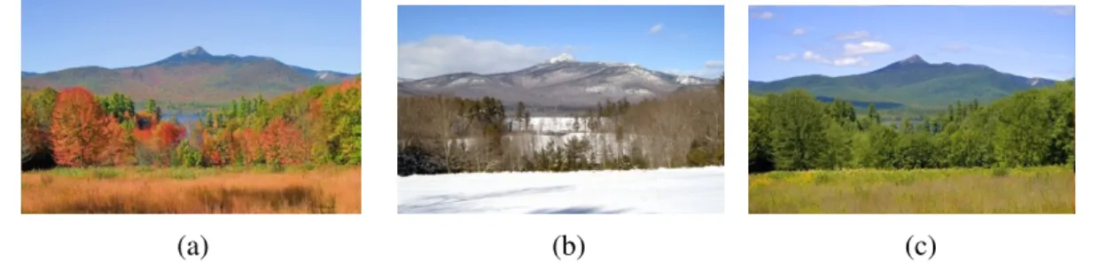
The time when an image was taken has a direct impact on many image attributes, such as transient attributes. Looking at an image of the same scene at different times as in Fig-ure 3.2, you can notice the obvious changes in the image appearance from summer to fall, and then to winter. Similarly, different other attributes changing over time, for example, people wear different types of clothes at different times of the year. In an image captured in summer, we will see people wearing shorts and t-shirts, whereas in winter they wear coats

(27)

Figure 3.3: Visual appearance changes dramatically due to differences in location and time. Our work takes advantage of sparsely distributed, ground-level image data, with associated location and time metadata, in conjunction with overhead imagery to construct dynamic maps of visual appearance attributes.

and jackets. Another interesting nonvisual attribute of an image that got less attention is the sound that you could hear at an image’s environment. If you were asked to predict the type of sounds you could hear in the environment of an image of a city that was taken at daytime, you will probably predict noisy and crowded sounds. Whereas if you were asked to predict the sound for another image of the same city taken at night, you will probably predict less noisy sounds.

3.3 General Framework for Mapping

Different works in computer vision have proposed approaches for constructing maps that show the differences of objects with respect to the image’s geolocations. Hayes et al. [25] proposed a method for mapping images appearance to geolocation. Other proposed meth-ods for mapping people’s visual appearance [10, 28]. Other works proposed methmeth-ods for mapping different geospatial attributes from ground-level images including household

(28)

in-come, education level, crime statistics, housing prices, and population density [4, 19]. Recently, different works have been proposed for estimating ground-level attributes from overhead imagery. Lee et al. [35] proposed an approach to estimate geo-informative attributes such as population density and demographic properties. Another work by Song et al. [58] proposed a method to estimate a road segment’s free-flow speed from over-head imagery and road metadata. Similar to our approaches, the work in [70] proposed a method for mapping between ground-level and overhead image and utilized the proposed method for the problem of image localization. But these methods ignore the fact that many attributes change not only over geolocation but also continuously changing over time.

In this work, we propose a general framework for image-driven mapping. In partic-ular, we propose a cross-modal distillation strategy to learn to predict the distribution of fine-grained properties from overhead imagery, without requiring any manual annota-tion of overhead imagery. With this strategy, we are able to estimate probability distri-butions over categories that would normally be considered too difficult for overhead im-agery understanding, due to the lack of available training data. By using large numbers of GPS-tagged consumer photographs, we use off-the-shelf networks including image classi-fication, scene classiclassi-fication, and weather condition estimation in ground-level images to build a sparse training dataset for overhead image understanding. Different ground-level attributes change for many reasons including the time and geolocation. Therefore, our framework has the option to integrate the time and geolocation for constructing dynamic maps.

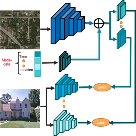
Figure 3.3 shows an overview of our architecture. We first construct a feature embed-ding for each conditioning variable (time, location, overhead image) using a set ofcontext

neural networks (top left). We combine these context features to predict the visual at-tributes that are coming from the co-located ground-level images usingestimatornetworks (top right). On the bottom left, we have a set of pre-trained networks that extract visual attributes from the ground-level images. These networks are only used for extracting visual attributes, which are used to train the context and estimator networks.

Our proposed approach has several advantages.

• it does not require any manually annotated training data.

• it can model spatiotemporal trends, without the need for overhead imagery at every time.

• it is extendable to a wide range of visual attributes.

In the next chapters, we demonstrate the effectiveness of our general framework on map-ping different ground-level attributes including places, objects, weather conditions, and sounds.

(29)

Chapter 4 Learning Static Maps of Visual

Appearance

4.1 Introduction

Traditional approaches to pixel-level labeling of remote sensed imagery rely on the manual specification of semantic categories. In our view, this limits the ability to predict categories for which a human annotator has low confidence. This means that we are unable to learn to make predictions about less certain categories. We propose to overcome this problem using a weakly-supervised learning strategy that uses manually specified labels in a domain for which humans are confident (ground-level imagery) but allows us to make less confident predictions for overhead imagery. With this strategy we are able to estimate probability distributions over categories that would normally be considered too difficult for overhead imagery understanding, due to the lack of available training data.

In particular, using large numbers of GPS-tagged consumer photographs, we use off-the-shelf networks for image classification, scene classification, and object detection in ground-level images to build a sparse training dataset for overhead image understanding. We extend the approach in [70] by modeling the distribution of labels. The previous work assumed that the predictions of the ground-level images were distributed in a Gaussian manner, and only learned to predict the mean of the distribution. This is problematic when a particular overhead image could have multiple possible interpretations from a ground-level perspective. For example, if the overhead image contains a beach and a parking lot, then the ground-level image may be of a beach or a parking lot, depending on the orientation.

(30)

as samples from a Dirichlet distribution. We use a multi-task approach and predict the parameters of prior distributions over three label spaces: scene categorization [79], image classification [32], and object detection [49].

4.2 Related Work

Many recent works jointly reason about ground-level and overhead image viewpoints. Zhai et al. [77] incorporate a transformation between co-located ground-level and overhead im-ages to learn semantic features for overhead imagery. Cross-view image geolocalization strategies [38, 39, 69, 70] learn a feature mapping between the two viewpoints in order to leverage densely available overhead imagery. Other works have used large-scale image collections to map properties of the world. For example, Lee et al. [35] estimate geo-informative attributes such as population density and demographic properties. Another work by Salem et al. [52] proposed an approach for constructing an aural atlas, which captures the geospatial distribution of soundscapes. Most similar to our work, Workman et al. [70] proposed an approach for cross-view training to learn similar feature representation for co-located ground and overhead images and use this for geolocalization. Greenwell et al. [23] proposed a similar cross-view learning approach to learn a model that is capable of predicting the type and count of objects that are likely to be seen from a ground-level per-spective conditioned on the overhead image. The previous two methods work on a single ground-level distribution. We propose a general architecture that can learn all labels that we can get from the ground perspective.

4.3 Approach

We propose a cross-view training strategy (Figure 4.1) that uses pre-existing CNNs to ex-tract categorical distributions of ground-level images to provide a weak signal for predict-ing the parameters of probabilistic models conditioned on co-located overhead imagery. We simultaneously learn three such probabilistic models that model separate ground-level distributions (Places categories, ImageNet categories, and MS-COCO object counts).

4.3.1 Dataset

In our work, we use the5.518 51×105 _{Flickr geotagged ground-level images contained in} the Cross-View USA (CVUSA) dataset [70]. For each ground-level image, we extracted two categorical distributions: one over 365-Places categories using a VGG16-Places365

(31)

Figure 4.1: An overview of our network architecture.

scene recognition model trained on Places2 [79], and another over 1.000×103_-Objects categories using VGG16-Imagenet trained for the task of image classification [32]. We also use the constructed histogram describing the objects present in each image following the work of Greenwell et. al. [23] that uses the output of Faster R-CNN ResNet 101 [49] detector trained on the MS-COCO challenge dataset [40]. To train our model, we split our data into93%training,2%validation, and5%testing.

4.3.2 Distribution Representation

We use two common distribution functions to model priors over ground-level image dis-tributions: Dirichlet and Poisson. The Dirichlet distribution is the conjugate prior of the categorical distribution, meaning samples drawn from a Dirichlet distribution are them-selves categorical distributions. Given parameters αi, the probability density function is given by the following equation:

f(x1, ..., xk;α1, ..., αk) = 1 B(α) k Y i=1 xαi−1 i (4.1)

whereB(α)is a normalizing constant. Using this we can model the one-to-many relation-ship between overhead imagery and potential ground-level scene and object probabilities

(32)

through a discrete set of parameters.

The Poisson distributions describe the likelihood of an event happeningktimes in some fixed interval. In our case, this will be the probability ofk objects of a class being present in the spatial extent of the scene. For each object class, the probability of k objects of that class appearing is given by the following equation, whereλis the interval rate, which varies per class.

P(k) = e−λλ

k

k! (4.2)

Using a Poisson distribution, we can directly model probabilities of not only the types of objects expected in a ground-level scene, but also the number of expected occurrences.

4.3.3 Network Architecture

Our network (Figure 4.1) has two main components, the first is a collection of pre-trained models that we use for extracting ground-level predictions. The second is a shared CNN which takes an overhead image as input and produces a feature which is passed to3 sepa-rate prediction heads. These heads sepasepa-rately predict 1) parameters of a Dirichlet distribu-tion over Places scene categories, 2) parameters of a Dirichlet distribudistribu-tion over ImageNet classes, and 3) parameters of Poisson distributions over the histogram of objects in the image for each overhead image. Each head consist of two fully connected layers. The first layer of each head contains1024neurons. The second layer is different for each task, 365, 1.000×103, and 91respectively. During training we use three losses, one for each distribution, that minimize the mean negative log-likelihood of the resulting probability distributions as in the following equations:

L=min 1

N

X

a

−log(p(g|a, w)) (4.3) whereg represents the distribution coming from the ground-level image,ais the overhead imagery, andwthe learned weights .

4.3.4 Implementation Details

Our model is implemented in TensorFlow. We trained ResNet-v2-50 [27] using the cross-view learning approach as in [52]. Specifically, the model is trained to predict distributions over ground-level scene and Imagenet categories from overhead imagery using the KL-divergence as a loss function. The trained ResNet is then frozen for subsequent training of the three prediction heads. The heads are initialized randomly using Xavier initialization.

(33)

(a) (b)

Figure 4.2: For a given ground image, we show the top-3 overhead images that give the highest probability for the given image. The top row is based on Places, the second on Imagenet, and the last on Object counts.

We optimize each head simultaneously by minimizing the negative log-likelihood (Equa-tion 4.3). For both ResNet pre-training and training of the predic(Equa-tion heads, we use the Adam optimizer with a learning rate of 0.001 and a weight decay factor of 0.0005 for 6 epochs with batch size32. The input images are re-sized to224×224, scaled to[−1,1], and augmented by random horizontal and vertical flipping.

4.4 Evaluation

We evaluated our learned models quantitatively and qualitatively on the test-set defined in the Dataset section.

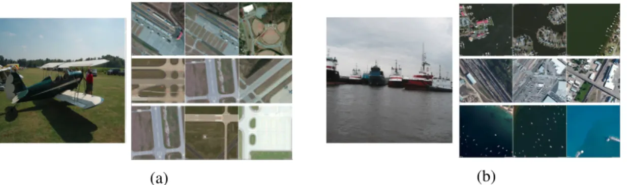
4.4.1 Cross-View Image Retrieval

For a given overhead image, we extract the output parameters to define the three distribu-tions. The distributions are used to compute the log-probability for any given ground-level image to identify the top-3 overhead images with highest probability. Two qualitative ex-amples are shown in Figure 4.2. The right image shows the ground-level image and on the left we show the top-3 overhead-images for each distribution. For example, in (a) the top row shows overhead images covering Baseball field andhighwayswhere in the middle and bottom coveringrunways.

4.4.2 Cross-View Localization

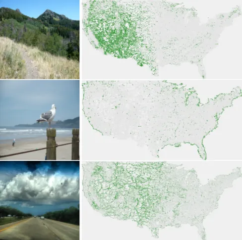
Our model can be used for ground-level image localization by defining the distributions for every overhead image in a reference dataset based on the predicted parameters. In Fig-ure 4.3, we took4.882 24×105_{overhead images from CVUSA. For each overhead image,}

(34)

Figure 4.3: Given a query ground-level image (left), we can construct a heatmap (right) that represents the score where the greener the dot on the map the more likely the image was taken in that location.

we predict the Places-Dirichlet distributions and, for any ground-level image, get a score for each reference image. The heatmap represents the score, where the greener the dot, the more likely the image was taken in that location. In the middle row, our method clearly identifies the image as having been captured in the coast of USA. Here we show results based on the Places-Dirichlet distribution, but the other two distribution can be used in the same way.

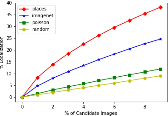
4.4.3 Localization Accuracy

We evaluated the accuracy of our learned probabilistic models on the task of localization. In Figure 4.4 the y-axis represents the accuracy and the x-axis is k, where top-k represents that the correct geolocation for the ground-level image appears ink%of the overhead im-ages. We can see that using the distribution based on Places gives the highest accuracy and the worst performance (but still better than random) is based on the Poisson distribution.

(35)

Figure 4.4: Localization accuracy of the different learned probabilistic models on the test-set of the ground-level imagery

Figure 4.5: Overhead images with the highest scores for thecarlabel. Theparklabel score is increased from left to right, transitioning the images from industrial to rural scenes while focusing on roads. Each column represents multiple images with similar scores for the query labels.

(36)

We suspect this is due to the fact that most of the 91 labels used to train the predicted pa-rameters for the Poisson distribution are difficult to learn from the overhead imagery, such as the labelstop sign.

4.4.4 Multi-Attribute Region Search

We find the geolocation based on the output images that give a high score for a search query attribute. For example, In Figure 4.5, images with the highest score forcar(an ImageNet label) are given, with increasing score forpark (a Places label) from left to right. While each image is centered around a large road, they transition from industrial to rural as the

parkscore increases.

4.5 Conclusion

We created a location-dependent model of geo-place understanding conditioned on over-head imagery. We show how our model can be used to generate maps at varying spatial scales. In the future, we will extend this work to include time, because what you can expect to see and experience at a location are highly dependent on time.

(37)

Chapter 5 Learning Dynamic Maps of Visual

Appearance

5.1 Introduction

Through experience, humans develop an understanding of the relationship between time, location, and the visual appearance of a scene. We learn to know, for example, when to expect it to be dark, whether a scene will likely contain snow, and where to stand for the best sunset. While this common sense, geo-visual understanding has many practical uses, relatively little research in the computer vision community has explored the problem. In this work, we present an important step towards the construction of a computational model of geo-visual understanding. Potential uses of our framework include verifying the integrity of image metadata, geolocalizing images, providing advice to photographers in search of a beautiful sunset, and enabling further studies of the relationship between the visual environment and health [53].

The field of computer vision has traditionally focused on the problem of extracting visual attributes of scenes captured from a human perspective. For example, categoriz-ing the scene type [79], estimatcategoriz-ing weather conditions [33], or predictcategoriz-ing demographic properties [19]. Recently, there has been a significant interest in the problem of image geolocalization, i.e., estimating the geographic location of the camera, or an object in the scene, given visual attributes extracted from the image. Solving this problem requires two elements: the ability to extract the visual attributes and an understanding of the geospatial distribution of these visual attributes. This naturally leads to the problem of image-driven mapping, in which we extract visual attributes from images with known geolocation and use these to construct a map of visual appearance.

(38)

Figure 5.1: Visual appearance changes dramatically due to differences in location and time. Our work takes advantage of sparsely distributed, ground-level image data, with associated location and time metadata, in conjunction with overhead imagery to construct dynamic maps of visual appearance attributes.

A map can be thought of as a probability distribution, conditioned on geographic lo-cation, over an attribute; typical attributes include land cover, land use, elevation, or place name. In this work, we propose to construct a map of visual attributes of the world. These attributes change for many reasons, including seasonal changes in plants and illumination changes due to the diurnal cycle. Therefore, we propose to build a dynamic map, which is a probability distribution conditioned on geographic location and time. The visual at-tributes of a ground-level image, such as those shown in Figure 5.1, are samples from this distribution.

We collect a large number of GPS-tagged and time-stamped images, extract visual features, and then learn to predict distributions over these features based on when and where the picture was captured. Directly predicting these features from geographic location alone is difficult because of the complexity of the distribution. We find that including the overhead image as a conditioning variable results in significantly better predictions. This is a promising approach because many features that relate the appearance of a place are

(39)

visible from above and high-resolution overhead imagery is available across the globe and is updated at increasing frequencies, some providers even promise daily updates [47].

In our work, we focus primarily on two visual attributes: the scene category [79], such as whether the image views an attic or a zoo, and transient attributes [33], which consists of time-varying properties such as sunny and foggy. We selected these because they are well known, easy to understand, and have very different spatiotemporal characteristics. The former is relatively stable over time, but can change rapidly with respect to location, especially in urban areas. The latter has regular, dramatic changes throughout the day and with respect to the season.

Contribution The key contribution of this work is a novel approach for image-driven mapping. Our approach has several advantages: it does not require any manually annotated training data; it can model differences in visual attributes at large and small spatial scales; it captures spatiotemporal trends, but does not require overhead imagery at every time; and is extendable to a wide range of visual attributes. We demonstrate the effectiveness of our approach through evaluation on large datasets for several different tasks. In each case, our model, which combines overhead imagery and metadata, is superior.

5.2 Related Work

A significant amount of research has sought to extract meaningful visual attributes from ground-level imagery. Dubey et al. [14] describe methods for quantifying the urban per-ception of safety, liveliness, wealth, and more. Laffont et al. [33] estimate attributes de-scribing scene appearance, such as if it is sunny or foggy. Other examples include in-terpreting weather conditions [41], estimating the local temperature [20], and predicting demographic properties [35]. When additional context about the imagery is known, such as the location or time of capture, these methods allow for characterizing properties of the underlying physical world.

Alternatively, studies have shown how additional image context can aid visual under-standing. Tang et al. [61] integrate the location an image was captured as an input to a framework for image classification and demonstrate improved results. Zhai et al. [78] de-scribe methods for learning geo-temporal features from location and time metadata. Wang et al. [65] use location information along with weather conditions to learn a feature repre-sentation for facial attribute classification. Unique from these works, we explore integrat-ing location and time metadata with overhead imagery to produce high resolution dynamic maps of visual attributes.

(40)

Figure 5.2: An overview of our network architecture, which includes the network we train to predict visual attributes (left) and the networks we use to estimate visual attributes (right).

Typically image-based methods for generating maps of visual attributes start by ex-tracting information from large-scale geotagged image collections and then apply a form of smoothing, such as locally weighted averaging, to produce a map. For example, Lee et al. [35] estimate geo-informative attributes such as population density and elevation. Wang et al. [67] create maps of snowfall by automatically recognizing snowy scenes. Bessinger et al. [10] map the visual appearance of people across the globe using a large corpus of geo-tagged face imagery. In our work, we integrate location and time as additional context in the learning process and take advantage of overhead imagery to produce higher resolution maps. There are numerous other papers that use similar approaches [36, 66, 73].

Imagery captured from an overhead perspective has been shown to aid ground-level image understanding. Luo et al. [42] use overhead imagery as additional context to im-prove event recognition in ground-level photos. Overhead imagery has also been used to synthesize images from a ground-level perspective [13, 48, 77]. Another research area has explored using ground-level imagery as a form of weak supervision for learning about over-head imagery. For example, Zhai et al. [77] introduce a method for labelling overover-head im-agery by learning a semantic transformation between co-located ground-level and overhead images. Other studies have explored the joint understanding of the two modalities. For in-stance, learning a feature mapping between ground-level and overhead image viewpoints enables image localization in regions without nearby ground-level images [38, 39, 69, 70]. More recently, Workman et al. [71, 72] integrate nearby ground-level images to improve the prediction of semantic properties.

Most relevant to our work, overhead imagery has been used to improve image-driven mapping by enabling fine-grained higher resolution maps. Workman et al. [71] combine overhead and ground-level imagery to map the scenicness of a region. Salem et al. [52]

(41)

proposed a method for constructing maps of soundscapes by relating overhead image ap-pearance to geolocated sounds. Our work extends this area by integrating location and time metadata as input to our framework.

5.3 Problem Definition

Our objective is to construct a map that represents the expected appearance at any geo-graphic location and time. The expected appearance is defined using a set of visual at-tributes, which could be low level, such as a color histogram, or higher-level, such as the scene category. For a given visual attribute,a, such a map can be modeled as a conditional probability distribution,P(a|t, l), given the time,t, and location,l, of the viewer.

We assume we are given a set of images,{Ii}, each with associated capture time,{ti}, and geo-location metadata, {li}. We assume these images are captured from a ground-level viewpoint. Furthermore, we assume we have the ability to calculate, or estimate with sufficient accuracy, each visual attribute from all images. The computed visual attributes, {ai}, can be considered samples from the probability distribution, P(a|t, l), and used for model fitting.

5.4 Dynamic Visual Appearance Mapping

We present a general approach to constructing a visual appearance map that works well across a broad range of tasks. We refine the distribution described in the previous sec-tion by adding an addisec-tional condisec-tioning variable. In particular, we define a condisec-tional probability distribution,P(a|t, l, I(l)), whereI(l)is an overhead image of the geographic location,l. Critically, the overhead image is not dependent on the time. This means that an overhead image is not required for every timestamp, t, of interest. An overhead image is

required for each location, but this is not a significant limitation given the wide availability of high-resolution satellite and aerial imagery.

5.4.1 Network Architecture Overview

Our model uses a mixture of convolutional and fully-connected neural networks to map from the conditioning variables to the parameters of distributions over a visual attribute,

P(a|F(t, l, I(l); Θ)), where Θare the parameters of all neural networks. See Figure 5.2

for an overview of our complete architecture, which simultaneously predicts two visual attributes. From the left, we first construct a feature embedding for each conditioning

(42)

vari-able using a set ofcontext neural networks. We combine these context features to predict the visual attributes using a per-attribute,estimatornetwork. From the right, a set of pre-trained networks extract visual attributes from the ground-level images. These networks are only used for extracting visual attributes, which are used to train the context and estimator networks. The attribute estimation networks are not trained in our framework.

5.4.2 Network Architecture Details

We have defined a macro-architecture for training a dynamic visual appearance map. In the remainder of this section, we define the specific neural network architectures and hyper-parameters we used.

Visual AttributesWe focus on two visual attributes:Places[79], which is a categorical distribution over 3.65×102 scene categories, and Transient [33], which is a multi-label attribute with 4.0×101 _{values that each reflect the degree of presence of different} time-varying attributes, such as sunny, cloudy, or gloomy. To extract thePlacesattributes, we use the pre-trained VGG-16 [57] network. To extract the transient attributes, we use a ResNet-50 [27] model that we trained using the original Transient Attributes Dataset [33].

Context NetworksThe context networks encode every conditioning variable, i.e., time, geographic location, and overhead image, to a1.28×102_{-dimensional feature vector. For} the time and geolocation inputs, we use two similar encoding networks, consisting of three fully connected layers each. The first layer contains2.56×102 neurons, the second has 5.12×102 neurons, and the third 1.28×102 neurons. The geographic location is repre-sented in earth-centered earth-fixed coordinates, scaled to the range[−1,1]. The time is factored into two components: the month of the year and the hour of the day. Each is scaled to the range[−1,1]. For the overhead image, we use a ResNet-50 model to extract the2.048×103_{-dimensional feature vector from the last global average pooling layer. This} feature is passed to a per-attribute head. Each head consists of two fully connected layers that are randomly initialized using the Xavier scheme [21]. The layers of each head have 2.56×102 and1.28×102 neurons, respectively.

Estimator Networks For each visual attribute, there is a separate estimator network that directly predicts the visual attribute. These consist of fully-connected layers, each with a ReLU activation. The input for these is the concatenation of the outputs of the encoding networks. For each, the first two layers contain256and512neurons, respectively. The third layer represents the output, with the number of neurons depending on the visual attribute. In this case, there are365output neurons for thePlacesestimator, with asoftmax

(43)

Figure 5.3: The spatial distribution of the dataset. The green (red) dots represent the train-ing (testtrain-ing) data.

5.4.3 Implementation Details

We jointly optimize all estimator and context networks with losses that reflect the quality of our prediction of the visual attributes extracted from ground-level images, {Ii}. For thePlaces estimator, the loss function is the KL divergence between attributes estimated from the ground-level image and the network output. For the Transient head, the loss function is theL2 distance between the attribute and the network output. These losses are optimized separately using Adam [31] with mini-batches of size 3.2×101. We applied

L2 regularization with scale 5×10−4 and trained all models for 1.0×101 epochs with learning rate1×10−3.

All networks were implemented using TensorFlow [2] and will be shared with the com-munity. Input images are resized to224×224 and scaled to[−1,1]. We pre-trained the overhead context network to directly predictPlacesandImagenetcategories of co-located ground-level images, minimizing the KL divergence for each attribute. The weights are then frozen and only the added attribute-specific heads are trainable.

For extracting transient attributes from the ground-level images, we use the dataset in-troduced by the authors [33] and train a ResNet-50 network, minimizing theL2 distance. The weights were initialized randomly using the Xavier scheme. We trained the network using Adam [31] until convergence with learning rate 0.001 and batch size 64. The re-sulting model achieves a mean squared error (MSE) of 3.04%. This improves upon the approach from the original authors, which used hand-engineered features and achieved an MSE of 4.2%.

(44)

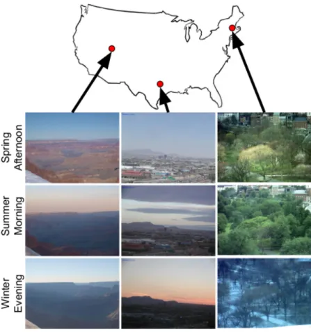
(a) Webcam Images

(b) Cell Phone Images

Figure 5.4: The temporal distribution of the dataset.

5.5 Evaluation

We evaluated our approach, both quantitatively and qualitatively, on a variety of tasks.

5.5.1 Dataset

We built an evaluation dataset by combining images from two sources. The first source is a set of images from the Archive of Many Outdoor Scenes (AMOS) [29], a collection of over a billion images captured from public outdoor webcams around the world. The sub-set [44] includes images captured between the years 2.013×103 and 2.014×103, from 5.0×101 webcams, totaling9.8633×104 images. Each image is associated with the lo-cation of the webcam and a timestamp (UTC) indicating when the image was captured. The second source is a subset of the Yahoo Flickr Creative Commons 100 Million Dataset (YFCC100M) [62]. This subset [78] contains only geotagged outdoor images, with time stamps, from smart phones. We combined both datasets to form a hybrid dataset containing

(45)

Table 5.1: Comparing performance on the visual attribute prediction task.

Context Transient (MSE) Places (KL)

loc 1.468 4.160 time 1.486 4.550 image 1.398 3.652 time+loc 1.239 3.897 image+loc 1.375 3.527 image+time 1.194 3.402 image+time+loc 1.159 3.300

3.050 11×105_images,₂_.₅₀₀₀_×₁₀4_{of which are held out for testing. For each image, we} also downloaded an orthorectified overhead image from Bing Maps (800×800, 0.60 me-ters/pixel), centered on the geographic location. Figure 5.3 shows the spatial distribution of the training (green dots) and testing images (red dots). Visual analysis of the distribution reveals that the images are captured from all over the world, with more images from Eu-rope and the United States. Further, examining the capture time associated with each image shows that the images cover a wide range of times. In Figure 5.4 (top), the distribution over month and hour for webcam images is essentially uniform, which is as anticipated because webcams are always on, capturing imagery at a standard interval. Figure 5.4 (bottom) shows the same visualization for cell phone images.

5.5.2 Baselines

For comparison, we trained several variants of our full model,image+time+loc. For each, we omit either one or two of the conditioning variables but keep all other aspects the same. We use the same training data, training approach, and micro-architectures. In total, we trained six baseline models:loc,image,time,time+loc,image+loc, andimage+time.

5.5.3 Prediction Accuracy

Using the testing set, we evaluate the prediction quality of our method and all baseline methods. Table 5.1 shows the errors for all approaches on both visual attributes. We find that our method has lower average error. However, the ranking of baseline models changes depending on the visual attribute. For example, the predictions for theimage+loc model are relatively worse for theTransient attribute than thePlacesattribute. This makes sense because the former is highly dependent on when an image was captured and the latter is more stable over time. We also note the significant improvement, for both attributes,

(46)

lush warm gloomy

January

April

July

Figure 5.5: Dynamic visual attribute maps for different transient attributes and months. In each, yellow (blue) corresponds to a higher (lower) value for the corresponding attribute. Each attribute exhibits unique spatial and temporal patterns, which closely match the au-thors’ personal travel experiences.

time+loc time+image time+loc+image

January

April

July

Figure 5.6: Dynamic visual attribute maps for different methods on the transient attribute

Learning to Map the Visual and Auditory World

UKnowledge

UKnowledge

Learning to Map the Visual and Auditory World

Learning to Map the Visual and Auditory World

Table of Contents

Chapter 1

Introduction

1.1

Image Driven Mapping

1.2

Mapping Using Overhead Imagery

1.3

Contributions

1.4

Dissertation Outline

Chapter 2

Technical Background

2.1

Learning with Convolutional Neural Networks

2.2

Transfer Learning

2.2.1

Fixed feature extractor

2.2.2

Domain Adaptation

2.2.3

Knowledge Distillation

Chapter 3

General Framework for Mapping

Geospatial Attributes

3.1

Estimating Images Attributes

3.2

Mapping Time-Variant Image Attributes

3.3

General Framework for Mapping

Chapter 4

Learning Static Maps of Visual

Appearance

4.1

Introduction

4.2

Related Work

4.3

Approach

4.3.1

Dataset

4.3.2

Distribution Representation

4.3.3

Network Architecture

4.3.4

Implementation Details

4.4

Evaluation

4.4.1

Cross-View Image Retrieval

4.4.2

Cross-View Localization

4.4.3

Localization Accuracy

4.4.4

Multi-Attribute Region Search

4.5

Conclusion

Chapter 5

Learning Dynamic Maps of Visual

Appearance

5.1

Introduction

5.2

Related Work

5.3

Problem Definition

5.4

Dynamic Visual Appearance Mapping

5.4.1

Network Architecture Overview

5.4.2