Machine Learning for Instance Segmentation

(1)

DISSERTATION

submitted to the

Combined Faculty of Natural Sciences and

Mathematics

of Heidelberg University, Germany

for the degree of

Doctor of Natural Sciences

Put forward by

Steffen Wolf Born in Munich, Germany

(2)

(3)

Machine Learning for Instance Segmentation

Referees: Prof. Dr. rer. nat. Fred A. Hamprecht Prof. Dr. rer. nat. Carsten Rother

(4)

(5)

Abstract

Volumetric Electron Microscopy images can be used for connectomics, the study of brain connectivity at the cellular level. A prerequisite for this inquiry is the automatic identification of neural cells, which requires machine learning algorithms and in particular efficient image segmentation algorithms.

In this thesis, we develop new algorithms for this task. In the first part we provide, for the first time in this field, a method for training a neural network to predict optimal input data for a watershed algorithm. We demonstrate its superior performance compared to other segmentation methods of its category.

In the second part, we develop an efficient watershed-based algorithm for weighted graph partitioning, theMutex Watershed, which uses negative edge-weights for the first time. We show that it is intimately related to the multicut and has a cutting edge performance on a connectomics challenge. Our algorithm is currently used by the leaders of two connectomics challenges [55,90].

Finally, motivated by inpainting neural networks, we create a method to learn the graph weights without any supervision.

(6)

(7)

Zusammenfassung

3D-Elektronenmikroskopbilder können für die Konnektomik, dem Studium der Neuron-verbindungen im Nervensystem, genutzt werden. Als Vorbereitung für diese Fragestellung nutzt man die automatische Identifizierung von Neuronen durch effiziente Bildsegmentierungsalgo-rithmen aus dem maschinellen Lernen.

In dieser Arbeit entwickeln wir neue Algorithmen für diese Aufgabe. Im ersten Teil stellen wir zum ersten Mal in diesem Forschungsgebiet eine Prozedur vor, die ein neuronales Netzwerk so trainiert, dass optimale Eingabedaten für einen Watershed Algorithmus bereitgestellt werden. Wir zeigen, dass diese Methode im Vergleich zu anderen Segmentierungsverfahren derselben Art bessere Resultate liefert.

Im zweiten Teil, entwickeln wir einen effizienten Algorithmus (denMutex Watershed) für das Partitionieren eines gewichteten Graphen. Dieser erlaubt zum ersten Mal die Verwendung neg-ativer Gewichte. Wir zeigen, dass derMutex Watershedeng mit demmulticutverwandt ist und zum Zeitpunkt der Veröffentlichung eine Spitzenposition in einer Konnektomik-Challenge ein-genommen hat. Unser Algoithmus is momentan Teil von zwei führenden Segmentierungsmeth-oden [55,90].

Zum Abschluss stellen wir eine Methode unter Nutzung von bildvervollständigenden neu-ronalen Netzwerken bereit, welche den gewichteten Graph ganz ohne Überwachung lernt.

(8)

(9)

Acknowledgments

First of all, I would like to thank Professor Fred A. Hamprecht, for sparking my passion for Machine Learning through his lectures and accompanying projects. As my superviser, he provided me with the resources and support to develop and explore my ideas and develop myself as a scientist. I enjoyed our intense and productive discussions, where he always challenged me to dig deeper. I am incredibly grateful for the pleasant environment that he procures, full of incredibly friendly, supportive, and intelligent people that made collaborating a pure joy. I especially want to thank Constantin Pape and Alberto Bailoni, who played an indispensable role in conceiving and understanding the Mutex Watershed. In this spirit, I also want to thank Lukas Schott and Yuyan Li for working so closely together with me and push the Watershed algorithms to their limits. I would also like to thank the senior group members Ullrich Köthe, Anna Kreshuk, Carsten Hauboldt, and Martin Schiegg for the guidance and helping me to get up on my science feet. In particular, I like to thank Ullrich Köthe for our in-depth discussions about image segmentation algorithms and his late-night support during my first paper.

I would also like to thank Jan Funke, who invited me to visit his group in Janelia, explored new ideas with me, and encouraged me to think about the bigger picture. I fondly remember the friendly atmosphere and intelligent discussions in his group that immediately made me feel at home. I also want to thank my close friend Stefan Richter who was always reliable in planing our eventing, but most importantly, as a supporter during stressful times. A special thanks goes to Barbara Werner for fighting our bureaucratic battles. I would also like to thank my official supervisor Carsten Rother for his interest in my project and valuable comments during my presentations.

Finally, I would like to thank Luka Smalinskaite for her love, support, and simply making my life better. Special thanks, of course, also goes to my parents for their continuous, unconditional support throughout my life.

(10)

(11)

1 Introduction

Understanding the content of digital images is one of the fundamental tasks of Computer vision. Typically, “understanding” means to find a transformation which maps images to a condensed description appropriate for further analysis. One example is the task of image classification, where the image has to be assigned to a specific element of a given set of classes. If a set of images and their corresponding class assignments are available, one can learn this transformation, thus extrapolating the assignment to new images. This learning-based image analysis, a part of Machine Learning, has become a common approach over a wide range of tasks. Notably, (convolutional) neural networks, as a way to parametrize these transformations, show remarkable performance. In some applications, they are on par with medical experts in skin cancer diagnosis [44] or even surpass humans on challenges such as ImageNet[134] where more than 14 millions of images have to be assigned to thousand different classes.

A deeper understanding of the content of an image can be expressed by finding objects in an image. This can be done in different ways. In the following we will focus on image segmenta-tion, which groups the image pixels into meaningful regions. While semantic segmentation is the assignment of each pixel to a discrete set of labels (e.g.{road, sky, tree, car,. . . }), instance segmentation groups pixel together and allows to distinguish between instances of the same class (e.g., assigning each car in the image to its own cluster). One notable example that we will discuss later is the instance segmentation of neuronal tissue images. Here, every pixel belongs to a neuron cell (i.e., we only have one class), which makes semantic segmentation not applicable. Instead, the image pixels have to be grouped such that each group contains only pixels of one neuron. In this work we introduce new algorithms for instance segmentation specifically tailored for neuron segmentation. The combination of both tasks, where pixels are to be grouped, and each group is assigned to a label is known as a semantic instance segmentation which we will address inChapter 4.

(16)

1.1 Machine Learning for Segmentation

Neural networks have demonstrated an incredible performance in many fields. This success was made possible by the development of specialized network architectures. For image analysis tasks, neural networks commonly are arranged in layers (referred to as multilayer perceptions) where the output of each neuron only depends on the neurons of the previous layer. The structure of these connections determines the architecture of the neural network. The most important architecture class for segmentation tasks are convolutional neural networks (CNNs), which arrange their neurons spatially and only form connections in their local neighborhoods. This drastically reduces the number of parameters in the network and is also desirable since these layers can be efficiently implemented using convolutional kernels.

To solve the task of semantic segmentation, a specialized CNN, the fully convolutional network (FCN) was designed, that laid the groundwork for further modern methods [99]. The FCN maps each pixel to a class by analyzing a patch centered on this pixel. A full segmentation can then be efficiently generated in a sliding-window procedure. This architecture was improved by using an encoder-decoder structure, called U-Net [132], and feature pyramids FPN [95] which have recently been extended to semantic instance segmentation [71]. Especially the U-Net has been particularly successful in biological applications [132] and is used repeatedly throughout this thesis.

In this thesis we will approach the task of instance segmentation by learning to predict the input weights for a graph-based segmentation algorithm, which we will review inSection 1.2. An alternative approach is given by detection-based instance segmentation, which can be divided into two steps. First, bounding boxes are detected that define the instances and then pixels inside each bounding box are assigned to the instance if they are within a predicted mask [54]. However these bounding boxes may overlap and thus produce overlapping segments which is not always desirable [72].

We will also investigate methods for dense instance segmentation where all pixels have to be assigned to exactly one cluster. In particular we will be present graph-based segmentation algorithms which in particular dominate the field of connectomics. One key aspect of their success was the use of Machine Learning to predict meaningful graph weights as an input for sophisticated graph partitioning algorithms. Very accurate graph weights can be learned by training an edge classifier that predicts the transitions between objects [89] or the use of a structured loss function that directly optimizes the segmentation performance [151]. In the following section we will briefly discuss a selection of graph partitioning algorithms that are commonly used in combination with learned graph weight estimators.

(17)

Kruskal’s Algorithm:

KA G(V, E),weightsw:E →_R+_:

A← ∅

for(i, j) =e∈Ein ascending order of wedo

if notconnected(i, j;A)then

A←A∪e

returnA

Algorithm 1: Kruskal’s Algorithm for constructing a minimal spanning tree A on the weighted graphG(V, E).

1.2 Graph-based Segmentation Algorithms

Here we explain the basic ideas and notation of graph-based segmentation algorithms, which will be frequently used in this thesis. In general, graph-based image segmentation methods represent the image as a graphG = (V, E)where each nodeu ∈ V corresponds to a pixel in the image. Nodes are connected by edges (u, v) ∈ E. A weightwe is associated with

each edgee∈Ebased on some property of the pixels that it connects, such as their image intensities, gradients or the output of an edge classifier (e.g. obtained by a neural network). Depending on the method and application, the graph might be only sparsely connected, for example as a grid graph or a graph with limited local neighborhood connectivity. In this thesis we will build upon segmentation algorithms, including the watershed, that are closely related to minimum spanning trees (MST) [47,177] on this graph and their construction algorithms. One example is Kruskal’s algorithm that constructs a MST by considering all edges in order of their weight, adding them to the tree if the incident nodes are not already connected. Here, we introduce the notation that connected(i, j;A)is true if there exists a pathπfromitojwhich completely lies in aA.

A segmentation can be derived from the tree by breaking the tree at the edges with large weights [177] or using sets of seed nodes that may not be connected which is known as seeded watershed [38,39,107,157]. This watershed segmentation can also be understood as a minimal energy solution to an energy minimization problem. Its objective function is a special case of the unifying power watershed energy minimization framework [37] which also encompasses the Random walker and Graph cuts [77].

These algorithms, however, can only ingest positive (attractive) weights and thus need an auxiliary input (e.g., seed points and thresholds) to partition the graph into clusters. In contrast to the above class of algorithms, this thesis will provide watershed algorithms which can also

(18)

deal with repulsive weights. Other methods like Multi-label variants [75] and QPBO [133] and correlation clustering [14, 67, 70, 172,173] can also use both attractive and repulsive interactions. However, only our new algorithm presented inChapter 3and correlation clustering (also known as multicut) can find the number of clusters implicitly and are therefore particularly suited for applications where the number of clusters is a-priori unknown. Since our algorithm and the multicut both minimize a similar objective function (seeSection 3.4) we present a formal definition of the minimum multicut as

y∗= arg min y∈{0,1}E X e∈E weye (1.1) subject to ye≤ X e0_∈_C_\{_e_} ye0 ∀C∈ cycles(G) ∀e∈C (1.2)

When the image is to be partitioned into semantically similar objects the graph can be aug-mented with additional semantic nodes and edges [63]. If one wants to no internal boundaries inside a semantic class this problem can be modeled as a Multiway cut:

y∗ = arg min y∈{0,1}E X e∈E weye (1.3) subject to ye≤ X e0_∈_C_\{_e_} ye0 ∀C ∈ cycles(G) ∀e∈C (1.4) X t∈T ytv=|T| −1, ifT =6 ∅,∀v∈V\T (1.5) ytt0 = 1, ∀t, t0 ∈T, t6=t0c, f (1.6) ytu+ytv ≥yuv, ∀uv ∈E, t∈T \ A (1.7) ytu+yuv ≥ytv, ∀uv∈E, t∈T (1.8) ytv+yuv≥ytu, ∀uv∈E, t∈T (1.9)

In case internal boundaries are desired, the constraints ofeq. (1.7)can be removed [81]. Solving both the multicut and Multiway cut is in general NP-hard since the set of constraints ineq. (1.2)

andeq. (1.4)are of exponential size. Therefore any exact solver will fail to scaling to large graphs [18]. In this work we will investigate a novel set of watershed algorithms that intimately relate to the multicut and Asymmetric Multiway Cut objective but can be efficiently solved on large graphs.

(19)

1.2.1 Segmentation for Connectomics

Figure 1.1: llustration of neuron reconstruction in theDrosophila melanogasterbrain. The neurons are reconstructed from serial section transmission EM (TEM) volumes (represented on the left) of the fruit fly brain (ventral view on the right). Individual neuron instances are shown, represented by different colors, on the EM slice with corresponding colors in the brain volume. Image taken from [183].

Graph-based segmentation algorithms have been particularly successful in connectomics, a field of neuroscience that strives to reconstruct the complete central nervous systems of animals and studies their neural wiring diagram. A necessary step towards this goal is the segmentation of neural tissue delineating individual neuron cells and revealing their 3D shapes. This process is known as neuron reconstruction. The neural tissue is commonly imaged using electron microscopy techniques (e.g., serial section transmission EM) that yield 3D image volumes. For example, the brain of an adultDrosophila melanogaster, with a volume of∼8·107µm3and comprising∼100,000 neurons has been imaged with nanometer resolution producing a dataset of 106 TB [183]. To study data-sets of this size, automated processing, especially automated segmentation, is paramount to not only reconstruct the complete neural wiring diagram but also study neuron morphology and ultra-structure.

One automatic method for neuron tracing, the flood-filling networks, uses a recurrent neural network to iteratively extend individual neurons [60]. Other approaches learn to predict affinity graph between voxels or supervoxels [89,152] and determine the segmentation as optimal cuts of this graph [6, 7, 20, 49, 105, 119, 120]. Almost all of the top submissions of the CREMI [26] and SNEMI3D [135] segmentation challenge predict these affinities directly using convolutional networks [89,163]. An alternative approach to the direct prediction of affinities was proposed by Lee et al. [90], who instead learn dense voxel embeddings via deep metric learning and derive affinities in the embedded space.

(20)

1.3 Contribution and Overview of this Thesis

The core of this thesis is a novel set of watershed algorithms, whose centerpiece, theMutex Watershed, is presented in Chapter 3 and extended to semantic instance segmentation in Chapter 4. This set extends the classical family of watershed algorithms operating on purely attractive graphs by including repulsive interactions and effectively obviating the need for explicit seeds. We investigate machine learning approaches for predicting input weights for classical and Mutex Watersheds, focusing especially on supervised end-to-end learning in Chapter 2 and fully unsupervised learning in Chapter 5. The following list gives a brief overview of each chapter’s content.

Chapter 2: We show how to train a the boundary map prediction jointly with the watershed computation. The estimator for the merging priorities is cast as a neural network that is convolutional (over space) and recurrent (over iterations). The latter allows the learning of complex shape priors and outperforms other seeded segmentation methods on the CREMI segmentation challenge.

Chapter 3: We propose a greedy algorithm for signed graph partitioning, theMutex Watershed. Unlike seeded watershed, the algorithm can accommodate not only attractive but also repulsive interactions, allowing it to find a previously unspecified number of segments without the need for explicit seeds or a tunable threshold. We also prove that this simple algorithm finds a global optimum of an objective function that is intimately related to the multicut / correlation clustering integer linear programming formulation.

Chapter 4: The link between Mutex Watershed and correlation clustering suggests that a similar Watershed algorithm for joint graph partitioning and labeling exists whose objective function closely relates to the Asymmetric Multiway Cut objective. We prove its existence by extending the Mutex Watershed and demonstrate on 3D electron microscopy images that this joint formulation outperforms a procedure which separately optimizes of the partitioning and labeling problems.

Chapter 5: Deep neural networks trained to inpaint partially occluded images show a deep understanding of image composition. We investigate how this implicit knowledge of image composition can be leveraged for a fully self-supervised generation of Mutex Watershed inputs and thus self-supervised segmentation. We evaluate our method on two microscopy image datasets to show that it reaches comparable segmentation performance to supervised methods.

(21)

2 Learned Watershed

Common pipelines for segmentation and super-pixel generation consist of a learned boundary predictor and an inference step (e.g. seeded watershed). The following work was motivated by the observation that small holes in the boundary map estimation can drastically reduce the segmentation accuracy of the seeded watershed. This effect may be most prevalent when the boundary estimation (often a neuronal network) is trained with an unstructured loss that penalizes every pixel individually. Although heuristics (e.g.using the distance transform trans-form [20]) may mitigate this problem, it can ultimately only be addressed through structured loss functions that take the inference method into account. In this chapter1, we present our approach to incorporate a neural network into the seeded watershed segmentation algorithm and train itend-to-end. Furthermore, this integration enablesadaptiveboundary prediction where predictions in the current iterations can be based on past decisions. Through a lesion study we show thatadaptiveprediction outperforms static baselines.

2.1 Introduction

The watershed algorithm is an important computational primitive in low-level computer vision. Since it does not penalize segment boundary length, it exhibits no shrinkage bias like multi-terminal cuts or (conditional) random fields and is especially suited to segment objects with high surface-to-volume ratio, e.g. neurons in biological images.

In its classic form, the watershed algorithm comprises three basic steps: altitude computation, seed definition, and region assignment. These steps are designed manually for each application of interest. In a typical setup, the altitude is the output of an edge detector (e.g. the gradient magnitude or the gPb detector [10]), the seeds are located at the local minima of the altitude image, and pixels are assigned to seeds according to the drop-of-water principle [39].

In light of the very successful trend towards learning-based image analysis, it is desirable to eliminate hand-crafted heuristics from the watershed algorithm as well. Existing work

1

This chapter is based on our paper [162], which was published in 2017. The results in this chapter represent the current state at the time of publication. The implementation and training of the deep neural network for the experiments of this chapter have been carried out by Lukas Schott and myself with many enjoyable days of pair programming.

(22)

shows that learned edge detectors significantly improve segmentation quality, especially when convolutional neural networks (CNNs) are used [16,34, 130,169]. We take this idea one step further and propose to learn altitude estimation and region assignment jointly, in an end-to-end fashion: Our approach no longer employs an auxiliary objective (e.g. accurate boundary strength prediction), but trains the altitude function together with the subsequent region assignment decisions so that the final segmentation error is minimized directly. The resulting training algorithm is closely related to reinforcement learning.

Our method keeps the basic sructure of the watershed algorithm intact: Starting from given seeds2, we maintain a priority queue storing the topographic distance of candidate pixels to their nearest seed. Each iteration assigns the currently best candidate to “its” region and updates the queue. The topographic distance is induced by an altitude function estimated with a CNN. Crucially, and deviating from prior work, we compute altitudeson demand, allowing their conditioning on prior decisions, i.e. partial segmentations. The CNN thus gets the opportunity to learn priors for likely region shapes in the present data. We show how these models can be trained end-to-end from given ground truth segmentations usingstructured learning. Our experiments show that the resulting segmentations are better than those from hand-crafted algorithms or unstructured learning.

2.2 Related Work

Various authors demonstrated that learned boundary probabilities (or, more generally, boundary strengths) are superior to designed ones. In the most common setting, these probabilities are defined on the pixel grid, i.e. on the nodes of a grid graph, and serve as input of anode-based watershed algorithm. Training minimizes a suitable loss (e.g. squared or cross-entropy loss) between the predicted probabilities and manually generated ground truth boundary maps in an unstructuredmanner, i.e. over all pixels independently. This approach works especially well with powerful models like CNNs. In the important application of connectomis (see section

2.6.3), this was first demonstrated by [59]. A much deeper network [34] was the winning entry of the ISBI 2012 Neuro-Segmentaion Challenge [12]. Results could be improved further by progress in CNN architectures and more sophisticated data augmentation, using e.g. U-Nets [130], FusionNets [126] or networks based on inception modules [20]. Clustering of the resulting watershed superpixels by means of the GALA algorithm [73,117] (using altitudes from [12] resp. [130]) or the lifted multicut [20] (using altitudes from their own CNN) lead to additional performance gains.

When ground truth is provided in terms of region labels rather than boundary maps, a suitable

2

Incorporating seed definition into end-to-end learning is a future goal of our research, but beyond the scope of this paper.

(23)

boundary map must be created first. Simple morphological operations were found sufficient in [130], while [20] preferred smooth probabilities derived from a distance transform starting at the true boundaries. Outside connectomics, [16] achieved superior results by defining the ground truth altitude map in terms of thevectordistance transform, which allows optimizing the prediction’s gradient direction and height separately.

Alternatively, one can employ the edge-basedwatershed algorithm and learn boundary probabilities for the grid graph’s edges. The corresponding ground truth simply indicates if the end points of each edge are supposed to be in different segments or not. From a theoretical perspective, the distinction between node- and edge-based watersheds is not very significant because both can be transformed into each other [109]. However, the algorithmic details differ considerably. Edge-based altitude learning was first proposed in [48], who used hand-crafted features and logistic regression. Subsequently, [152] employed a CNN to learn features and boundary probabilities simultaneously. Watershed superpixel generation and clustering on the basis of these altitudes was investigated in [185].

Learning with unstructured loss functions has the disadvantage that an error at a single point (node or edge) has little effect on the loss, but may lead to large segmentation errors: A single missed boundary pixel can cause a big false merger. Learning withstructuredloss functions, as advocated in this paper, avoids this by considering the boundaries in each image jointly, so that the loss can be defined in terms of segmentation accuracy rather than pointwise differences. Holistically-nested edge detection [76,169] achieves a weak form of this by coupling the loss at multiple resolutions using deep supervision. Such a network was successfully used as a basis for watershed segmentation in [27]. The MALIS algorithm [151] computes shortest paths between pairs of nodes and applies a correction to the highest edge along paths affected by false splits or mergers. This is similar to our training, but we apply corrections to root error edges as defined below. Learned, sparse reconstruction methods such as MaskExtend [104] and Flood-filling networks [60] predict region membership for all nodes in a patch jointly, performing region growing for one seed at a time in a one-against-the-rest fashion. In contrast, our algorithm grows all seeds simultaneously and competitively.

2.3 Mathematical Framework

The watershed algorithm is especially suitable when regions are primarily defined by their boundaries, not by appearance differences. This is often the case when the goal isinstance segmentation (one neuron vs. its neighbors) as opposed to semantic segmentation (neurons vs. blood vessels). In graphical model terms, pairwise potentials between adjacent nodes are crucial in this situation, whereas unary potentials are of lesser importance or missing altogether. Many real-world applications have these characteristics, see [37] and section2.6for examples.

(24)

We consider 4-connected grid graphsG = (V, E). The input image I : V → _RD _maps

all nodes to D-dimensional vectors of raw data. A segmentation is defined by a label image S :V → {1,2, . . . , n}specifying the region index or label of each node. The ground truth segmentation is calledS∗. Pairwise potentials (i.e. edge weights) are defined by an altitude function over the graph’s edges

f :E→_R (2.1)

where higher values indicate stronger boundary evidence. Since this paper focuses on how to learn f, we assume that a set of seed nodes M = {m1, . . . , mn} ⊂ V is provided by a

suitable oracle (see section2.6for details). The watershed algorithm determinesSby finding a mappingσ:V →M that assigns each node to the best seed so that

σ(w) =mi ⇒ S(w) =i (2.2)

Initially, node assignments are unknown (designated byλ) except at the seeds, where they are assumed to be correct: σ0(w) =    mi ifw=miwithS∗(mi) =i λ otherwise (2.3)

In this paper, we build upon theedge-basedvariant of the watershed algorithm [39,106]. This variant is also known aswatershed cutsbecause segment boundaries are defined by cuts in the graph, i.e. by the set of edges whose incident nodes have different labels. We denote the cuts in our solution as∂Sand in the ground truth as∂S∗.

LetΦ(m, w)denote the set of all paths from seedm to nodew. Then themax-arc topo-graphic distancebetweenmandwis defined as [45]

T(m, w) = min

φ∈Φ(m,w)maxe∈φ f(e) (2.4)

In words, the highest edge in a pathφdetermines the path’s altitude, and the path of lowest altitude determines the topographic distance. The watershed algorithm assigns each node to the topographically closest seed [129]:

σ(w) = arg min

m∈M

T(m, w) (2.5)

The minimum distance path from seedmto nodewshall be denoted byφm(w). This path is

not necessarily unique, but ties are rare and can be broken arbitrarily whenf(e)is a real-valued function of noisy input data.

(25)

It was shown in [39] that the resulting partitioning is equivalent to the minimum spanning forest (MSF) over seedsM and edge weights f(e). Thus, we can compute the watershed segmentation incrementally using Prim’s algorithm: Starting from initial seeds σ0, each iterationkfinds the lowest edge whose start pointukis already assigned, but whose end point

vkis not

uk, vk= arg min (u,v)∈E σk−1(u)6=λ, σk−1(v)=λ

f(e= (u, v)) (2.6)

and propagates the seed assignment fromuktovk:

σk(w) =    σk−1(uk) ifw=vk σk−1(w) otherwise (2.7)

In a traditional watershed implementation, the altitudef(e)is a fixed, hand-designed function of the input data

f(e) =ffixed(e|I) (2.8)

for example, the image’s Gaussian gradient magnitude or the “global Probability of boundary” (gPb) detector [10].

2.4 Joint Structured Learning of Altitude and Region

Assignment

We propose to use structured learning to train an altitude regressorf(e)jointlywith the region assignment procedure defined by Prim’s algorithm. We will discuss two types of learnable altitude functions: fstaticcomprises models that, once trained, only depend on the input image I, whereasfdynadditionally incorporates dynamically changing information about the current state of Prim’s algorithm.

2.4.1 Static Altitude Prediction

To find optimal parametersθof a modelfstatic(e|I;θ), consider how Prim’s algorithm proceeds: It builds a MSF which assigns each nodewto the closest seedmˆ =σ(w)by identifying the shortest pathφmˆ(w)frommˆ tow. Such a path can be wrong in two ways: it may cross∂S∗ and thus miss a ground truth cut edge, or it may end at a false cut edge, placing ∂Sin the interior of a ground truth region. More formally, we have to distinguish two failure modes: (i)

(26)

∂S∗ ∂S ∂S∗ ˜ f(e) =∞ ∂S ∂S∗ ∂S ∂S∗ ˜ f(e) =∞ ∂S ∂S∗ ∂S ∂S∗ ˜ f(e) =∞ ∂S ∂S∗ ∂S ∂S∗ ˜ f(e) =∞ ∂S ∂S∗ ∂S ∂S∗ ˜ f(e) =∞ ∂S ∂S∗ ∂S ∂S∗ ˜ f(e) =∞ ∂S ∂S∗ ∂S ∂S∗ ˜ f(e) =∞ ∂S ∂S∗ ∂S ∂S∗ ˜ f(e) =∞ ∂S ∂S∗ ∂S ∂S∗ ˜ f(e) =∞ ∂S ∂S∗ ∂S ∂S∗ ˜ f(e) =∞ ∂S ∂S∗ ∂S ∂S∗ ˜ f(e) =∞ ∂S ∂S∗ ∂S ∂S∗ ˜ f(e) =∞ ∂S ∂S∗ ∂S ∂S∗ ˜ f(e) =∞ ∂S ∂S∗ ∂S ∂S∗ ˜ f(e) =∞ ∂S ∂S∗ ∂S ∂S∗ ˜ f(e) =∞ ∂S ∂S∗ ∂S ∂S∗ ˜ f(e) =∞ ∂S ∂S∗ ∂S ∂S∗ ˜ f(e) =∞ ∂S ∂S∗ ∂S ∂S∗ ˜ f(e) =∞ ∂S ∂S∗ ∂S ∂S∗ ˜ f(e) =∞ ∂S ∂S∗ ∂S ∂S∗ ˜ f(e) =∞ ∂S ∂S∗ ∂S ∂S∗ ˜ f(e) =∞ ∂S ∂S∗ ∂S ∂S∗ ˜ f(e) =∞ ∂S ∂S∗ ∂S ∂S∗ ˜ f(e) =∞ ∂S ∂S∗ ∂S ∂S∗ ˜ f(e) =∞ ∂S ∂S∗ ∂S ∂S∗ ˜ f(e) =∞ ∂S ∂S∗ ∂S ∂S∗ ˜ f(e) =∞ ∂S ∂S∗ ∂S ∂S∗ ˜ f(e) =∞ ∂S ∂S∗ ∂S ∂S∗ ˜ f(e) =∞ ∂S ∂S∗ ∂S ∂S∗ ˜ f(e) =∞ ∂S ∂S∗ ∂S ∂S∗ ˜ f(e) =∞ ∂S ∂S∗ ∂S ∂S∗ ˜ f(e) =∞ ∂S ∂S∗ ∂S ∂S∗ ˜ f(e) =∞ ∂S ∂S∗ ∂S ∂S∗ ˜ f(e) =∞ ∂S ∂S∗ ∂S ∂S∗ ˜ f(e) =∞ ∂S ∂S∗ ∂S ∂S∗ ˜ f(e) =∞ ∂S ∂S∗ ∂S ∂S∗ ˜ f(e) =∞ ∂S ˆ m ω ω ˆ m∗ b) a)

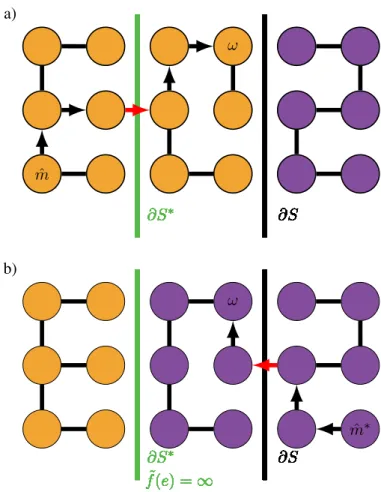
Figure 2.1: Example of root errors in the minimal spanning forest (a) and the constrained MSF (b) of a grid graph. Orange and purple indicate the segmentationSin (a) andS∗in (b). The root errorsρ(w)(top) andρ∗(w)(bottom) of a wrongly labeled nodeware marked red, with corresponding pathsφmˆ(w)andψm∗(w)depicted by arrows.

A node was assigned to the wrong seed, i.e.mˆ 6=m∗ =mS∗₍_w₎or (ii) it was assigned to the correct seed via a non-admissible path, i.e. a path taking a detour across a different region. To treat both cases uniformly, we construct the corresponding ground truth pathsψm∗(w).

These paths can be found by running Prim’s algorithm with a modified altitude

˜ f(e) =    ∞ ife∈∂S∗ fstatic(e|I;θ) otherwise (2.9)

(27)

forcing cuts in the resulting constrained MSF to coincide with∂S∗(see figure2.1). We denote the topographic distances alongφmˆ(w)andψm∗(w)asT( ˆm, w)andT∗(m∗, w)respectively. By construction of the MSF,φandψare equal for all correct nodes. Conversely, they differ for incorrect nodes, causing distanceT∗ to exceed distanceT. This property defines the setV−of

incorrect nodes:

V−={w:T∗(m∗, w)> T( ˆm, w)} (2.10)

Every incorrect pathφmˆ(w)contains at least one erroneous cut edge. The first such edge shall be called the path’srooterror edgeρ(w)and is always a missing cut. Training should increase its altitude until it becomes part of the cut set∂S. The root error edgeρ∗(w) of a ground truth pathψm∗(w)is the first false cut edge inψin failure mode (i) and the first edge whereψ deviates fromφin mode (ii). Here, the altitude should be decreased to make the edge part of the MSF, see figure2.1. Accordingly, we denote the sets of root edges asE↑ :={ρ(w) :w∈V−}

andE↓ :={ρ∗(w) :w∈V−}.

Since all assignment decisions in Prim’s algorithm are conditioned on decisions taken earlier, the errors in any path also depend on the path’s root error. Structured learning must therefore consider these errors jointly, and we argue that training updates must be derived solely from the root edges: They are the only locations whose required correction direction is unambiguously known. In contrast, we cannot even tell if subsequent errors will simply disappear once the root error has been fixed, or need updates of their own. When the latter applies, however, these edges will eventually become root errors in later training epochs, and we delay updating them to that point.

Since we need a differentiable loss to perform gradient descent, we use the perceptron loss of distance differences:

L=X

w

T∗(m∗, w)−T( ˆm, w) (2.11)

Correct nodes have zero contribution sinceT∗ =T holds for them. To serve as a basis for structured learning, we transform this into a loss over altitude differences at root edges. Since topographic distances equal the highest altitude along the shortest path, we have

T( ˆm, w)≥fstatic(ρ(w)) (2.12)

To derive similar relations forT∗, consider how the constrained MSF is constructed from the unconstrained one: First, edges crossing∂S∗are removed from the MSF. Each of the resulting orphaned subgraphs is then reconnected into the constrained MSF via the lowest edge not crossing∂S∗. The newly inserted edges are the root edgesρ∗of all their child nodes, i.e. all nodes in the respective subgraph. Since these root edges did not belong to the original MSF,

(28)

their altitude cannot be less than the maximum altitude in the corresponding child subgraph. Forw∈V−, it follows that

T∗(m∗, w) =fstatic(ρ∗(w)) (2.13)

We can therefore upper-bound the perceptron loss by

LSL=

X

w∈V−

fstatic(ρ∗(w))−fstatic(ρ(w))≥ L (2.14)

and minimize this upper bound. By rearranging the sum, the loss can be simplified into

L_SL(θ) =X

e∈E

R(e)fstatic(e|I;θ) (2.15)

where we introduced a weight function counting the children of each root edge

R(e) :=          P w:e=ρ∗₍_w₎1 ife∈E↓ −P w:e=ρ(w)1 ife∈E↑ 0 otherwise (2.16)

A training epoch of structured learning thus consists of the following steps:

1. Computefstatic(e|I;θ(t))andf˜(t)(e)with current model parametersθ(t)and determine the MSF and the constrained MSF.

2. Identify root edges and define the weightsR(t)(e)and the lossL(_SLt)(θ).

3. Obtain an updated parameter vectorθ(t+1)via gradient descent on∇_θL(t)_(θ)_at_θ₌_θ(t)_. These steps are iterated until convergence, and the resulting final parameter vector is denoted asθSL.

2.4.2 Relation to Reinforcement Learning

In this section we compare the structured loss functionLSLwith policy gradient reinforcement learning, which will serve as motivation for a refinement of the weighting functionR(e). To see the analogy, we refer to continuous control deep reinforcement learning as proposed by [94,142,147].

Looking at the region growing procedure from a reinforcement learning perspective, we define states as tupless= (e, I)wheree∈Eis the edge under consideration, and the action

(29)

spaceA:=Ris the altitude to be predicted byfstatic(e|I;θ). ThePolicy Gradient Theorem [147] defines the appropriate update direction of the parameter vectorθ. In a continuous action space, it reads ∇_θJ =∇_θX s dπ(s) Z A π(a|s;θ)Qπ(s, a) da (2.17)

whereJ is the performance to be optimized, dπ(s)the discounted state distribution, π the policy to be learned, andQthe action-value function estimating the discounted expected future reward Qπ(s, a) =Eπ h_XT t=0 γtrt a0=a, s0 =s;π i (2.18)

In our case, the state distribution reduces todπ(s) = _|_V1_| because Prim’s algorithm reaches each edge exactly once. Inserting our deterministic altitude prediction

π(a|s) :=fstatic(s|I;θ) δ(a−fstatic(s|I;θ)), (2.19) whereδis the Dirac distribution, we get

∇θJ = 1 |V|∇θ X s fstatic(s|I;θ)Qπ(s, a). (2.20)

Comparing equation (2.20) with equation (2.15), we observe that∇θJ ∼ ∇θLSL, where our weightsR(e)essentially play the role of the action-value functionQ. This suggests to introduce adiscount factorinR(e). To do so, we replace the temporal differencestbetween states in (2.18) with tree distances dist(w, ρ(w))or dist(w, ρ∗(w))counting the number of edges between nodewand its root edge. This gives the discounted weights

RRL(e) :=                P w:e=ρ∗₍_w₎ γdist(w, ρ∗(w)) ife∈E↓ P w:e=ρ(w) −γdist(w, ρ(w)) _if_e_∈_E ↑ 0 otherwise (2.21)

with discount factor0≤γ ≤1to be chosen such thatγdist_{decays roughly according to the} size of the CNNs receptive field. SubstitutingRRL(e)forR(e)in (2.15) significantly improves

convergence in our experiments. This analogy further motivates the application of current deep reinforcement training methods as described in section2.5.2.

(30)

2.4.3 Dynamic Altitude Prediction

In every iteration, region growing according to Prim’s algorithm only considers edges with exactly one end node located in the already assigned set. This offers the possibility to delay altitude estimation to the time when the values are actually needed. On-demand altitude computations can take advantage of the partial segmentations already available to derive additionalshapeclues that help resolving difficult assignment decisions.

Relative Assignments:To incorporate partial segmentations, we remove their dependence on the incidental choice of label values by means oflabel-independent projection. Consider an edgee= (u, v)where nodeuis assigned to seedmand nodevis unassigned. We now construct a labeling relative tom, distinguishing nodes assigned tom(“me” region), to another seed (“them”) and unassigned (“nobody”). Relative labelings are represented by a standard 1-of-3 coding: P(w|m, σ) =          (1,0,0) ifσ(w) =m (me) (0,1,0) ifσ(w) =λ (nobody) (0,0,1) otherwise (them) (2.22)

In practice, we process relative labelings by adding a new branch to our neural network that receivesP as an input, see section2.5.1for details.

Non-Markovian modeling: Another potentially useful cue is afforded by the fact that Prim’s algorithm propagates the assignments recursively. Thus during every evaluation off the complete history from previous iterations along the growth pathsφmcan be incorporated. We

encode the historyH : V →_Rr_{about past assignment decisions as an}_r_{-dimensional vector}

in each node. In practice, we incorporate history by adding a recurrent layer to our neural network.

We introduce thedynamicaltitude predictions: f(e= (u,v)),H(v) =

fdyn(e|I,P(.|σ(u), σ),H(u);θdyn) (2.23) that receives the relative assignments projectionP andu’s hidden stateH(u)as an additional input and outputs both the edge’s altitudef(e)andv’s hidden stateH(v): This variant of the altitude estimator performs best in our experiments. The emergent behavior of our models suggests that the algorithm uses history to adjust local diffusion parameters such as preferred direction and “viscosity”, similar to the viscous watershed transform described in [156].

(31)

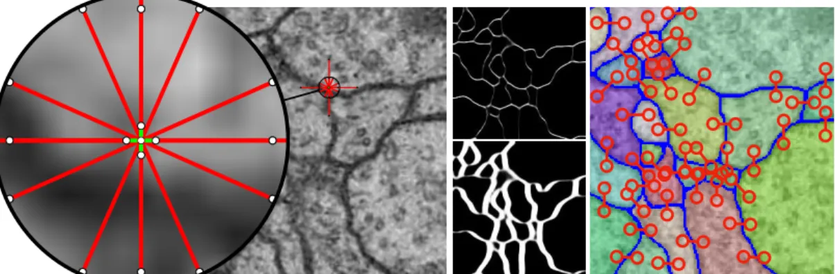
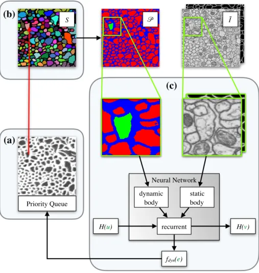
fdyn(e) Priority Queue S 𝒫 Ĩ dynamic body static body recurrent Neural Network H(u) H(v)

(a)

(b)

(c)

Figure 2.2: Overview implementation of learned watershed algorithm with neural network and priority queue. In each iteration the minimal edge according to equation (2.6) is found using a priority queue (a) and the region label is propagated (b), which updates the projectionP. For all unassigned edges that are not in the priority queue and need to be considered by Prim’s algorithm in the next iteration, the altitudefdyn(e)is evaluated using the dynamic

(32)

2.5 Methods

2.5.1 Neural Network Architecture

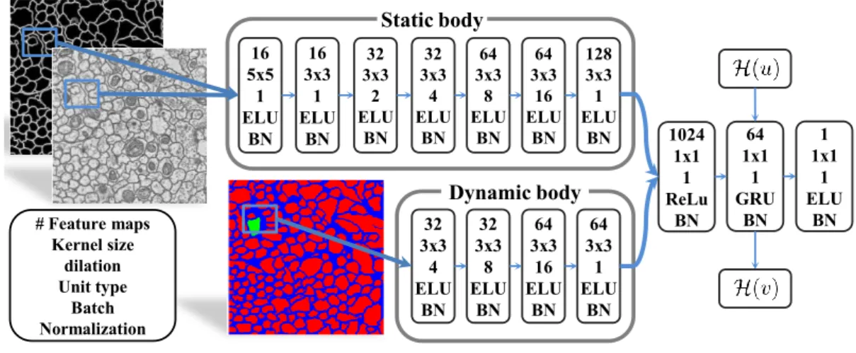
Our network architecture builds mainly on the work of Yu and Koltun [175] who introduced dilated convolutions to achieve dense segmentations and systematically aggregate multi-scale contextual information without pooling operations. We split our network into two convolutional branches (see Figure2.3): The upper branch processes the static inputI, and the lower one the dynamic inputP(·). Since the input of the upper branch doesn’t change during prediction, its network activations can be precomputed for all edges, leading to a significant speed-up. We choose gated recurrent units (GRU) instead of long short-term memory (LSTM) in the recurrent network part, because GRUs have no internal state and get all history from the hidden state vectorH(·), saving on memory and bookkeeping.

2.5.2 Training Methods

Augmenting the Input Image:We noted above that structured learning is superior because it considers edges jointly. However, it can only rely on the sparse training setsE↓∪E↑. In

contrast, unstructured learning can make use of all edges and thus has a much bigger training set. This means that more powerful predictors, e.g. much deeper CNNs, can be trained, leading to more robust predictions and bigger receptive fields.

To combine the advantages of both approaches, we propose to augment the input imageI with an additional channel holding node boundary probabilities predicted by an unstructured modelg(w|I;θUL):

˜

I := [I g] :V →_RD+1 (2.24)

We train the CNNgseparately beforehand and replaceIwith theaugmented inputI˜everywhere infstaticandfdyn. This simplifies structured learning because the predictor only needs to learn a refinement of the already reasonable altitudes ing. In principle, one could even trainf andg jointly, but the combined model is too big for reliable optimization.

Training Schedule:Taking advantage of the close relationship with reinforcement learning, we adopt the asynchronous update procedure proposed by [110]. Here, independent workers fetch the current CNN parametersθfrom the master and compute loss gradients for randomly selected training images in parallel. The master then applies these updates to the parameters in an asynchronous fashion. We found experimentally, that this lead to faster and more stable convergence than sequential training.

In order to train the recurrent network part, we replace the standard temporal input ordering with the succession of edges defined by the pathsφandψ. In a sense, backpropagation in time thus becomes backpropagation along the minimum spanning forest.

(33)

Static body Dynamic body 16 5x5 1 ELU BN 16 3x3 1 ELU BN 32 3x3 2 ELU BN 32 3x3 4 ELU BN 64 3x3 8 ELU BN 64 3x3 16 ELU BN 128 3x3 1 ELU BN 32 3x3 4 ELU BN 32 3x3 8 ELU BN 64 3x3 16 ELU BN 64 3x3 1 ELU BN 1024 1x1 1 ReLu BN 64 1x1 1 GRU BN 1 1x1 1 ELU BN # Feature maps Kernel size dilation Unit type Batch Normalization

Figure 2.3: Neural Network architecture: The static body extracts features from the raw input and edge detector output. The more shallow dynamic body processes the interactions of different region projectionsP. These informations are combined in a fully connected layer and set into a temporal context using a recurrent GRU layer. The network output is the priority of the edge towards the pixel at the center of the field of view.

2.6 Experiments and Results

Our experiments illustrate the performance of our proposed end-to-end trainable watershed in combination with static and dynamic altitude prediction. To this end, we compare with standard watershed and power watershed algorithms [37] on statically trained CNNs according to [20], see section2.6.2. Furthermore we show in section2.6.3that the learned watershed surpasses the state-of-the-art segmentation in an adapted version of the CREMI Neuron Segmentation Challenge [26].

2.6.1 Experimental Setup and Evaluation Metrics

Seed Generation Oracle: All segmentation algorithms start at initial seeds M which are here provided by a “perfect” oracle. In our experiments, this oracle uses the ground truth segmentation to select one pixel with maximalL2distance to the region boundary per ground truth region.

Segmentation Metrics: In accordance with the CREMI challenge [26], we use the fol-lowing segmentation metrics: The Rand scoreVRandmeasures the probability of agreement between segmentationSand ground truthS∗ w.r.t. a randomly chosen node pairw, w0. Two segmentations agree if both assignwandw0 to the same region or to different regions. The

(34)

Rand error ARAND= 1−VRand_{is the opposite, so that smaller values are better.}

TheVariation of Information(VOI)betweenSandS∗is defined asV OI(S;S∗) =H(S|S∗)+ H(S∗|S),whereHis the conditional entropy [103]. To distinguish split errors from merge er-rors, we report the summands separately as VOISPLIT=H(S|S∗)and VOIMERGE=H(S∗|S)

2.6.2 Artificial Data

a) b) c) d)

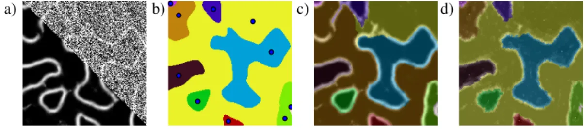
Figure 2.4: Artificial data example. a) Raw withσnoise= 0.6and prediction of baseline CNN. b) Ground

truth. c) The brown region leaks out when standard watershed runs on top of baseline CNN. d) Our algorithm uses learned shape priors to close boundary gaps.

Dataset: In order to compare our modelsfstaticandfdynwith solutions based on unstructured learning, we create an artificial segmentation benchmark dataset with variable difficulty. First, we generate an edge image via the zero crossing of a 2D Gaussian process. This image is then smoothed with a Gaussian filter and corrupted with Gaussian noise atσnoise∈ {0.3,0.6,0.9}. For eachσnoise, we generate 1900 training images and 100 test images of size 252x252. One test image with corresponding ground truth and results is shown in figure2.4.

Baseline: We choose a recent edge detection network from [175] to predict boundaries between different instances in combination with standard watershed (WS) and Power Watershed (PWS) [37] to generate an instance segmentation. Since these algorithms work best on slightly smoothed inputs, we apply Gaussian smoothing to the CNN output. The optimal smoothing parameters are determined by grid search on the training dataset. Additionally, we apply all watershed methods directly to smoothed raw image and report their overall best result asRAW + WS.

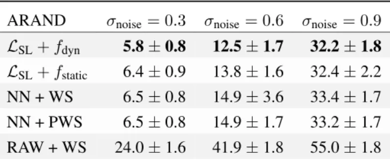
Performance: The measured segmentation errors of all algorithms are shown in table

2.1. Observed differences in performance mainly indicate how well each method handles low-contrast edges and narrow gaps between regions. The structurally trained watersheds outperform the unstructured baselines, because our loss functionLSL heavily penalizes the resulting segmentation errors. In all experiments, thedynamic predictionfunctionfdynhas the best performance, due to its superior modeling power. It can identify holes and close most contours correctly because it learns to derive shape and contingency clues from monitoring

(35)

ARAND σnoise= 0.3 σnoise= 0.6 σnoise= 0.9 L_SL+fdyn 5.8±0.8 12.5±1.7 32.2±1.8 LSL+fstatic 6.4±0.9 13.8±1.6 32.4±2.2 NN + WS 6.5±0.8 14.9±3.6 33.4±1.7 NN + PWS 6.5±0.8 14.9±1.7 33.2±1.7 RAW + WS 24.0±1.6 41.9±1.8 55.0±1.8

Table 2.1: Quality of the segmentation results on the artificial dataset. Reported lowest error for all parameters of baseline watersheds based on the rand error and a two pixel boundary distance tolerance.

intermediate results during the flooding process. A representative example of this effect is shown in figure2.4.

2.6.3 Neurite Segmentation

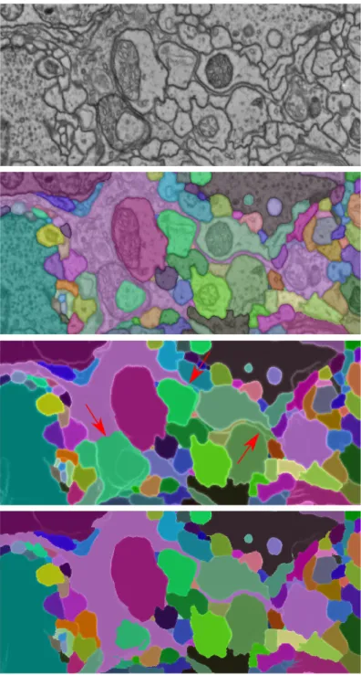
Dataset: The MICCAI Challenge on Circuit Reconstruction from Electron Microscopy Im-ages [26] contains 375 fully annotated slices of electron microscopy imagesI (of resolution 1250x1250 pixels). Part of a data slice is displayed in figure2.6top. Since the test ground truth segmentation has not been disclosed, we generate a new train/test split from the 3 origi-nal challenge training datasets by spltnting them into 3x75 z-continuous training- and 3x50 z-continuous test blocks.

Ideally, we would compare with [20] whose results define the state-of-the-art on the CREMI Challenge at time of submission. However, their pipeline, as described in their supplementary material, optimizes 2D segmentations jointly across multiple slices with a complex graphical model, which is beyond the scope of this paper.

Instead, we isolate the 2D segmentation aspect by adapting the challenge in the following manner: We run each segmentation algorithm with fixed ground truth seeds (see section2.6.1) and evaluate their results on eachz-slice separately. The restriction to 2D evaluation requires a slight manual correction of the ground truth: The ground truth accuracy inz-direction is just

±1slice. The official 3D evaluation scores compensate for this by ignoring deviations of±1 pixels inz-direction. Since this trick doesn’t work in 2D, we remove 4 regions with no visual evidence in the image and all segments smaller than 5 pixels. Boundary tolerances in the x-y plane are treated as in the official CREMI scores where deviations from the true boundary are ignored if they do not exceed 6.25 pixels.

(36)

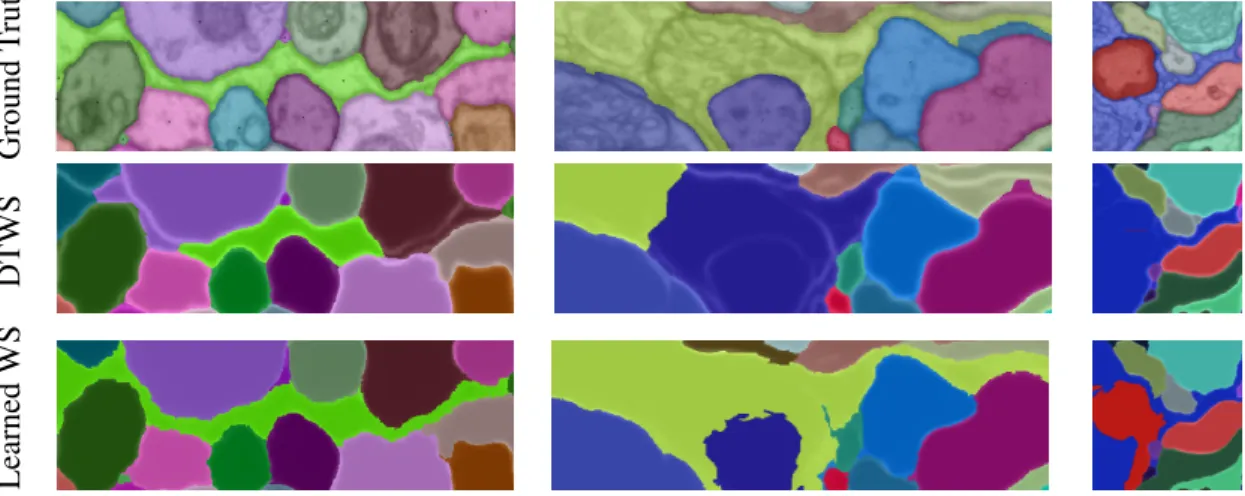
Ground T ruth DTWS Learned WS

Figure 2.5: Detailed success and failure cases of our method. Success case: long thin neurites (left), weak boundaries (middle). Failure case (right).

[37], Viscous Watershed [156], RandomWalker [50], Stochastic Watershed [9] and Distance Transform Watershed [20]. The boundary probability predictiong(the samegas in equation (2.24)) was provided by a deep CNN trained with an unstructured loss-function. In particular, the Distance Transform Watershed (DTWS) and the predictiongwere used to produce the current state-of-the-art on the CREMI challenge. To obtain the DTWS, one thresholds g, computes a distance transform of the background, i.e. the non-boundary pixels and runs the watershed algorithm on the inverted distances. According to [20], this is the best known heuristic to close boundary gaps in these data, but requires manual parameter tuning. We found the parameters of all baseline algorithms by grid search using the training dataset. To ensure fair comparison, we start region growing from ground truth seeds in all cases. Our algorithm takes the augmented imageI˜fromeq. (2.24)as input and learns how to close boundary gaps.

Comparison to state-of-the-art:We show the 2D CREMI segmentation scores inTable 2.2. It is evident that the learned watershed transform significantly outperforms DTWS in both ARAND and VOI score. Quantitatively, we find that the flooding patterns and therefore the region shapes of the learned watershed prefer to adhere to biologically sensible structures. We illustrate this with our results on one CREMI test slice inFigure 2.6, as well as specific examples in Figure 2.5. We find throughout the dataset that especially thin processes, as depicted in the left panel ofFigure 2.5, are a strength of our algorithm. Biologically sensible shape completionscan also be found for roundish objects and is particularly noticeable when boundary evidence is weak, as shown inFigure 2.5center. However, in rare cases, we find

(37)

ARAND VOI split VOI merge PowerWS 0.122±0.003 0.340±0.031 0.180±0.019 ViscousWS 0.093±0.003 0.328±0.030 0.069±0.003 RandomWalker 0.103±0.004 0.355±0.037 0.060±0.004 Stochastic WS 0.193±0.012 0.612±0.080 0.077±0.004 DTWS 0.085±0.001 0.320±0.029 0.070±0.005 Learned WS 0.082±0.001 0.319±0.030 0.057±0.004

Table 2.2: CREMI segmentation metrics evaluated on 2D slices: The Variation of Information (VOI) between a predicted segmentation and ground truth (lower is better) and the Adapted Rand Error (lower is better) [12].

incorrect shape completions (see right panel ofFigure 2.5), mainly in areas of weak boundary evidence. It stands to reason that these errors could be fixed by providing more training data.

2.7 Conclusion

This paper proposes an end-to-end learnable seeded watershed algorithm that performs well an artificial data and neurosegmentation EM images. We found the following aspects to be critical success factors: First, we train a very powerful CNN to control region growing. Second, the CNN is trained in a structured fashion, allowing it to optimize segmentation performance directly, instead of treating pixels independently. Third, we improve modeling power by incorporating dynamic information about the current state of the segmentation. Specifically, feeding the current partial segmentation into the CNN provides shape clues for the next assignment decision, and maintaining a latent history along assignment paths allows to adjust growing parameters locally. We demonstrate experimentally that the resulting algorithm successfully solves difficult configurations like narrow region parts and low-contrast boundaries, where previous algorithms fail. In future work, we plan to include seed generation into the end-to-end learning scheme.

(38)

Figure 2.6: From top: Raw data. Ground truth. Result of distance transform WS (red arrows point out major errors). Result of our algorithm.

(39)

3 Mutex Watershed

In this chapter1, we present our approach to incorporate repulsive interactions into the wa-tershed algorithm. We show that this is beneficial in practice, obviating the need for seed prediction2. Furthermore, we prove that this simple algorithm finds a global optimum of an objective function that is intimately related to the multicut / correlation clustering integer linear programming formulation. When presented with short-range attractive and long-range repulsive cues from a deep neural network, the Mutex Watershed gives the best results currently known for the competitive ISBI 2012 EM segmentation benchmark.

3.1 Introduction

Most image partitioning algorithms are defined over a graph encoding purely attractive inter-actions. No matter whether a segmentation or clustering is then found agglomeratively (as in single linkage clustering / watershed) or divisively (as in spectral clustering or iterated normal-ized cuts), the user either needs to specify the desired number of segments or a termination criterion. An even stronger form of supervision is in terms of seeds, where one pixel of each segment needs to be designated either by a user or automatically. Unfortunately, clustering with automated seed selection remains a fragile and error-fraught process, because every missed or hallucinated seed causes an under- or oversegmentation error. Although the learning of good edge detectors boosts the quality of classical seed selection strategies (such as finding local minima of the boundary map, or thresholding boundary maps), non-local effects of seed placement along with strong variability in region sizes and shapes make it hard for any learned predictor to placeexactly oneseed in every true region.

In contrast to the above class of algorithms, multicut / correlation clustering partitions

1

This chapter is based on our paper [163,165], which was published in 2018/2019. The results in this chapter rep-resent the current state at the time of publication. The algorithm was implemented and conceived by Constantin Pape and myself, whose neural network training pipeline for EM-images segmentation was indispensable for beating the state-of-the-art on the ISBI challenge. The theoretical characterization of the algorithm was done by Alberto Bailoni and me. Alberto especially developed the relation of the MWS to the Power watershed framework.

2

Seed prediction for neuron segmentation is usually infeasible, due to the large, complex structures of the segments that also lack unique identification points.

(40)

vertices with both attractive and repulsive interactions encoded into the edges of a graph. Multicut has the great advantage that a “natural” partitioning of a graph can be found, without needing to specify a desired number of clusters, or a termination criterion, or one seed per region. Its great drawback is that its optimization is NP-hard.

The main insight of this paper is that when both attractive and repulsive interactions between pixels are available, then a generalization of the watershed algorithm can be devised that segments an imagewithoutthe need for seeds or stopping criteria or thresholds. It examines all graph edges, attractive and repulsive, sorted by their weight and adds these to an active set iff they are not in conflict with previous, higher-priority, decisions. The attractive subset of the resulting active set is a forest, with one tree representing each segment. However, the active set can have loops involving more than one repulsive edge. See Fig.3.1for a visual abstract.

In summary, our principal contributions are, first, a fast deterministic algorithm for graph partitioning with both positive and negative edge weights that does not need prior specification of the number of clusters (section3.4); and second, its theoretical characterization, including proof that it globally optimizes an objective related to the multicut correlation clustering objective (3.4).

Combined with a deep net, the algorithm also happens to define the state-of-the-art in a competitive neuron segmentation challenge (Section 3.5).

This is an extended version version of [163], with the second principal contribution (section

3.4) being new.

Figure 3.1: Left: Overlay of raw data from the ISBI 2012 EM segmentation challenge and the edges for which attractive (green) or repulsive (red) interactions are estimated for each pixel using a CNN. Middle: vertical / horizontal repulsive interactions at intermediate / long range are shown in the top / bottom half. Right: Active mutual exclusion (mutex) constraints that the proposed algorithm invokes during the segmentation process.

(41)

3.2 Related Work

In the original watershed algorithm [22,157], seeds were automatically placed at all local minima of the boundary map. Unfortunately, this leads to severe over-segmentation. Defining better seeds has been a recurring theme of watershed research ever since. The simplest solution is offered by the seeded watershed algorithm [23]: It relies on an oracle (an external algorithm or a human) to provide seeds and assigns each pixel to its nearest seed in terms of minimax path distance.

In the absence of an oracle, many automatic methods for seed selection have been proposed in the last decades with applications in the fields of medicine and biology. Many of these approaches rely on edge feature extraction and edge detection like gradient calculation [4, 124]. Other types of methods generate seeds by first performing feature extraction [125,166], whereas others first extract region of interests and then place seeds inside these regions by using thresholding [3], binarization [140],k-means [111] or other strategies [1,2].

In applications where the number of regions is hard to estimate, simple automatic seed selection methods, e.g. defining seeds by connected regions of low boundary probability, do not work: The segmentation quality is usually insufficient because multiple seeds are in the same region and/or seeds leak through the boundary. Thus, in these cases seed selection may be biased towards over-segmentation (with seeding at all minima being the extreme case). The watershed algorithm then produces superpixels that are merged into final regions by more or less elaborate postprocessing. This works better than using watersheds alone because it exploits the larger context afforded by superpixel adjacency graphs. Many criteria have been proposed to identify the regions to be preserved during merging, e.g. region dynamics [51], the waterfall transform [21], extinction values [155], region saliency [115], and(α, ω)-connected components [144]. A merging process controlled by criteria like these can be iterated to produce a hierarchy of segmentations where important regions survive to the next level. Variants of such hierarchical watersheds are reviewed and evaluated in [123].

These results highlight the close connection of watersheds to hierarchical clustering and minimum spanning trees/forests [108, 113], which inspired novel merging strategies and termination criteria. For example, [137] simply terminated hierarchical merging by fixing the number of surviving regions beforehand. [101] incorporate predefined sets of generalized merge constraints into the clustering algorithm. Graph-based segmentation according to [47] defines a measure of quality for the current regions and stops when the merge costs would exceed this measure. Ultrametric contour maps [10] combine the gPb (global probability of boundary) edge detector with an oriented watershed transform. Superpixels are agglomerated until the ultrametric distance between the resulting regions exceeds a learned threshold. An optimization perspective is taken in [52,69], which introducesh-increasing energy functions and builds the hierarchy incrementally such that merge decisions greedily minimize the energy.

(42)

The authors prove that the optimal cut corresponds to a different unique segmentation for every value of a free regularization parameter.

An important line of research is given by partitioning of graphs with both attractive and repulsive edges [66]. Solutions that optimally balance attraction and repulsion do not require external stopping criteria such as predefined number of regions or seeds. This generaliza-tion leads to the NP-hard problem of correlageneraliza-tion clustering or (synonymous) multicut (MC) partitioning. Fortunately, modern integer linear programming solvers in combination with incremental constraint generation can solve problem instances of considerable size [8], and good approximations exist for even larger problems [119,172] Reminiscent of strict minimizers [91] with minimalL∞-norm solution, our work solves the multicut objective optimally when

all graph weights are raised to a large power.

Related to the proposed method, the greedy additive edge contraction (GAEC) [65] heuristic for the multicut also sequentially merges regions, but we handle attractive and repulsive interactions separately and define edge strength between clusters by a maximum instead of an additive rule. The greedy fixation algorithm introduced in [92] is closely related to the proposed method; it sorts attractive and repulsive edges by their absolute weight, merges nodes connected by attractive edges and introduces no-merge constraints for repulsive edges. However, similar to GAEC, it defines edge strength by an additive rule, which increases the algorithm’s runtime complexity compared to the presented Mutex Watershed. Also, it is not yet known what objective the algorithm optimizes globally, if any.

Another beneficial extension is the introduction of additional long-range edges. The strength of such edges can often be estimated with greater certainty than is achievable for the local edges used by watersheds on standard 4- or 8-connected pixel graphs. Such repulsive long-range edges have been used in [179] to represent object diameter constraints, which is still an MC-type problem. When long-range edges are also allowed to be attractive, the problem turns into the more complicated lifted multicut (LMC) [56]. Realistic problem sizes can only be solved approximately [19,65], but watershed superpixels followed by LMC postprocessing achieve state-of-the-art results on important benchmarks [20]. Long-range edges are also used in [89], as side losses for the boundary detection convolutional neural network (CNN); but they are not used explicitly in any downstream inference.

In general, striking progress in watershed-based segmentation has been achieved by learning boundary maps with CNNs. This is nicely illustrated by the evolution of neurosegmentation for connectomics, an important field we also address in the experimental section. CNNs were introduced to this application in [59] and became, in much refined form [34], the winning entry of the ISBI 2012 Neuro-Segmentation Challenge [12]. Boundary maps and superpixels were further improved by progress in CNN architectures and data augmentation methods, using U-Nets [130], FusionNets [126] or inception modules [20]. Subsequent postprocessing with the GALA algorithm [73, 117], conditional random fields [154] or the lifted multicut [20]

(43)

pushed the envelope of final segmentation quality. MaskExtend [104] applied CNNs to both boundary map prediction and superpixel merging, while flood-filling networks [60] eliminated superpixels altogether by training a recurrent neural network to perform region growing one region at a time.

Most networks mentioned so far learn boundary maps on pixels, but learning works equally well for edge-based watersheds, as was demonstrated in [121,185] using edge weights gener-ated with a CNN [151,152]. Tayloring the learning objective to the needs of the watershed algorithm by penalizing critical edges along minimax paths [151] or end-to-end training of edge weights and region growing [162] improved results yet again.

Outside of connectomics, [16] obtained superior boundary maps from CNNs by learning not just boundary strength, but also its gradient direction. Holistically-nested edge detection [76, 169] couples the CNN loss at multiple resolutions using deep supervision and is successfully used as a basis for watershed segmentation of medical images in [27].

We adopt important ideas from this prior work (hierarchical single-linkage clustering, at-tractive and repulsive interactions, long-range edges, and CNN-based learning). The proposed efficient segmentation framework can be interpreted as a generalization of [101], because we also allow for soft repulsive interactions (which can be overridden by strong attractive edges), and constraints are generated on-the-fly.

3.3 The Mutex Watershed Algorithm as an Extension of

Seeded Watershed

In this section we introduce the Mutex Watershed Algorithm, an efficient graph clustering algorithm that can ingest both attractive and repulsive cues. We first reformulate seeded watershed as a graph partitioning with infinitely repulsive edges and then derive the generalized algorithm for finitely repulsive edges, which obviates the need for seeds.

3.3.1 Definitions and notation

Let G = (V, E, w)be a weighted graph. The scalar attributew : E → _Rassociated with each edge is a merge affinity: the higher this number, the higher the inclination of the two incident vertices to be assigned to the same cluster. Conversely, large negative affinity indicates a greater desire of the incident vertices to be in different clusters. In our application, each vertex corresponds to one pixel in the image to be segmented. We call an edgee∈Erepulsive ifwe <0and we call it attractive ifwe>0and collect them inE−={e∈E|we<0}and