Boredom and student modeling in intelligent tutoring systems

(1)

Worcester Polytechnic Institute

Digital WPI

Masters Theses (All Theses, All Years) Electronic Theses and Dissertations

2014-04-25

Boredom and student modeling in intelligent

tutoring systems

William J. Hawkins

Worcester Polytechnic Institute

Follow this and additional works at:https://digitalcommons.wpi.edu/etd-theses

This thesis is brought to you for free and open access byDigital WPI. It has been accepted for inclusion in Masters Theses (All Theses, All Years) by an authorized administrator of Digital WPI. For more information, please [email protected].

Repository Citation

Hawkins, William J., "Boredom and student modeling in intelligent tutoring systems" (2014).Masters Theses (All Theses, All Years). 307. https://digitalcommons.wpi.edu/etd-theses/307

(2)

BOREDOM AND STUDENT MODELING IN INTELLIGENT TUTORING

SYSTEMS

by

William Joseph Hawkins

A Thesis

Submitted to the Faculty

of the

WORCESTER POLYTECHNIC INSTITUTE

in partial fulfillment of the requirements for the

Degree of Master of Science

in

Computer Science

April 2014

APPROVED:

_______________________________

Dr. Neil T. Heffernan, Advisor

_______________________________

Dr. Sonia Chernova, Thesis Reader

_______________________________

Dr. Craig Wills, Head of Department

(3)

ii

Abstract

Over the past couple decades, intelligent tutoring systems (ITSs) have become popular in education. ITSs are effective at helping students learn (VanLehn, 2011; Razzaq, Mendicino & Heffernan, 2008; Koedinger et al, 1997) and help researchers understand how students learn. Such research has included modeling how students learn (Corbett & Anderson, 1995), the effectiveness of help given within an ITS (Beck et al, 2008), the difficulty of different problems (Pardos & Heffernan, 2011), and predicting long-term outcomes like college attendance (San Pedro et al, 2013a), among many other studies.

While most studies have focused on ITSs from a cognitive perspective, a growing number of researchers are paying attention to the motivational and affective aspects of tutoring, which have been recognized as important components of human tutoring (Lepper et al, 1993). Recent work has shown that student affect within an ITS can be detected, even without physical sensors or cameras (D’Mello et al, 2008; Conati & Maclaren, 2009; Sabourin et al, 2011; San Pedro et al, 2013b).

Initial studies with these sensor-less affect detectors have shown that certain problematic affective states, such as boredom, confusion and frustration, are prevalent within ITSs (Baker et al, 2010b). Boredom in particular has been linked to negative learning outcomes (Pekrun et al, 2010; Farmer & Sundberg, 1986) and long-term disengagement (Farrell, 1988). Therefore, reducing or responding effectively to these affective states within ITSs may improve both short- and long-term learning outcomes.

This work is an initial attempt to determine what causes boredom in ITSs. First, we determine which is more responsible for boredom in ITSs: the content in the system, or the students themselves. Based on the findings of that analysis, we conduct a randomized controlled trial to determine the effects of monotony on student boredom. In addition to the work on boredom, we also perform analyses that concern student modeling, specifically how to improve Knowledge Tracing (Corbett & Anderson, 1995), a popular student model used extensively in real systems like the Cognitive Tutors (Koedinger et al, 1997) and in educational research.

(4)

iii

Acknowledgements

I would like to thank my advisors, Neil T. Heffernan and Ryan S.J.d. Baker, for the time and effort they dedicated to advising me on the work contained here and in general.

I would like to thank Neil and Cristina Heffernan for creating the ASSISTments system and for helping me understand it better. Thanks to Cristina for help with constructing and running the randomized controlled trial.

I would like to thank the ASSISTments lab for helping me understand the system and providing me with the data I needed.

For applying the affect detectors to data sets and helping me understand how they work, I would like to thank Supreeth Gowda and Maria San Pedro.

For coauthoring one of the published papers that comprise this thesis and giving advice on other parts of it, I would like to thank Yutao Wang.

I would like to thank Lisa Rossi for proofreading Chapter 2 of this thesis before it was published. I would like to thank Professors Joseph Beck and Ivon Arroyo and all the students that attended the weekly Educational Data Mining research meetings for sharing their expertise and giving valuable feedback on my work. Thanks to Xiaolu Xiong for organizing these meetings.

This work was funded by Graduate Assistance in Areas of National Need (GAANN) and Partnership in Math and Science Education (PIMSE) fellowships, a CAREER grant, the National Science Foundation (#1316736, #1252297, #1109483, #1031398, #0742503), ONR's 'STEM Grand Challenges,’ IES (# R305A120125 & R305C100024) and grant #OPP1048577 from the Bill & Melinda Gates Foundation.

Many other funders of the ASSISTments system are listed at

(5)

iv

Table of Figures

Figure 1: Example of a student working through a problem in ASSISTments. ... 6

Figure 2: Example of a “light bulb” question in ASSISTments. ... 13

Figure 3: Example of a histogram question whose cover story is about heights of trees in California’s Redwood Forest. ... 14

Figure 4: Possible questions sequences for students in each condition. ... 15

Figure 5: Examples of assistance within ASSISTments (from Wang and Heffernan, 2011) ... 21

Figure 6: Static Bayesian network representation of Knowledge Tracing ... 22

Figure 7: Example of the Empirical Probabilities method... 39

Table of Tables

Table 1: Model fitting results for state vs. trait. R2 calculated using five-fold cross-validation, BiC’ calculated over the entire dataset ... 8

Table 2: Model fitting results for fatigue. Models including both fatigue and other factors given at bottom. ... 9

Table 3: Model fitting results for type and skill ... 10

Table 4: Average confidence of each affective state for each condition, first averaged within each student, then averaged across all students... 16

Table 5: Average confidence of each affective state split by condition and previous performance. ... 17

Table 6: Average confidence of each affective state split by condition and previous performance. ... 17

Table 7: AM table for entire dataset ... 24

Table 8: Initial APM table for the entire dataset ... 25

Table 9: APM table for the entire dataset ... 26

Table 10: Example dataset ... 27

Table 11: Results for the individual models ... 28

Table 12: Results for the mean models ... 30

Table 13: Results for the linear regression models ... 31

Table 14: Results for the decision tree models ... 32

Table 15: Results for averaging the KT and random forest models ... 33

Table 16: Results for the best of each ensembling method ... 33

Table 17: Significance tests for the best ensembling methods ... 34

Table 18: Prediction results for the two methods of learning BKT parameters: Expectation Maximization and Empirical Probabilities ... 40

(8)

1

Chapter 1: Introduction

Over the past couple decades, intelligent tutoring systems (ITSs) have become popular in education. Used in a variety of environments with various age groups for various purposes, ITSs give students individual attention they do not get in the classroom, and feedback they do not get from traditional pencil-and-paper assignments. Several studies have shown the effectiveness of ITS (VanLehn, 2011; Razzaq, Mendicino & Heffernan, 2008; Koedinger et al, 1997).

In addition to helping students, ITSs have helped researchers learn about how students learn. Such research has included modeling how students learn (Corbett & Anderson, 1995), the effectiveness of help given within an ITS (Beck et al, 2008), the difficulty of different problems (Pardos & Heffernan, 2011), and predicting long-term outcomes like college attendance (San Pedro et al, 2013a), among many other studies.

While most studies have focused on ITSs from a cognitive perspective, a growing number of researchers are paying attention to the motivational and affective aspects of tutoring, which have been recognized as important components of human tutoring (Lepper et al, 1993). Recent work has shown that student affect within an ITS can be detected, even without physical sensors or cameras (D’Mello et al, 2008; Conati & Maclaren, 2009; Sabourin et al, 2011; San Pedro et al, 2013b). This is important because it allows for affect detection to be much more scalable, given the high cost and short lifespans of physical sensors in school environments.

Initial studies with these sensor-less affect detectors have shown that certain problematic affective states, such as boredom, confusion and frustration, are prevalent within ITSs (Baker et al, 2010b). Boredom in particular has been linked to negative learning outcomes (Pekrun et al, 2010; Farmer & Sundberg, 1986) and long-term disengagement (Farrell, 1988). Therefore, reducing or responding effectively to these affective states within ITSs may improve both short- and long-term learning outcomes.

This work is an initial attempt to determine what causes boredom in ITSs. The second chapter is a published analysis that sets out to determine which is more responsible for boredom in ITSs: the content in the system, or the students themselves. Based on the findings of that analysis, the unpublished work in the third chapter involves a randomized controlled trial whose purpose is to determine the effects of monotony on student boredom. In addition to the work on boredom, the fourth and fifth chapters of this work are published conference papers that both concern student modeling, specifically how to improve Knowledge Tracing (Corbett & Anderson, 1995), a popular student model used extensively in real systems like the Cognitive Tutors (Koedinger et al, 1997) and in educational research. Chapters 2, 4 and 5 appear in this thesis as they did when they were originally published, except for formatting and table and figure numbers for the sake of consistency throughout the document, and the acknowledgements and references for each have been pooled together in the respective sections of this document.

(9)

2

All of the work presented here was done using the ASSISTments system (Feng, Heffernan & Koedinger, 2009), a free web-based platform used primarily for middle- and high-school mathematics. Developed at Worcester Polytechnic Institute in collaboration with Carnegie Mellon University, ASSISTments was used by approximately 60,000 students during the 2013-2014 school year.

(10)

3

Chapter 2: Determining the main cause of boredom in intelligent tutoring

systems

Boredom is unpleasant, and has been repeatedly shown to be associated with poor performance and long-term disengagement in educational contexts. Boredom is prevalent within a range of online learning environments, has been shown to correlate negatively with learning in those environments, and often precedes disengaged behaviors such as off-task behavior and gaming the system. Therefore, it is important to identify the causes of boredom in these environments. In psychology research, there is ongoing debate about the degree to which individual students are prone to boredom (“trait” explanations) or the degree to which boredom is driven by state-based factors, such as the design of the learning environment. In this study, we apply an unobtrusive computational detector of student boredom to log data from an intelligent tutoring system to determine whether state or trait factors better predict the prevalence of boredom in students using that system. Knowing which type of factor better predicts boredom in a specific system can help us to narrow down further research on why boredom occurs and what steps should be taken to mitigate boredom’s negative effects.

This chapter was published at the following venue:

Hawkins, W., Baker, R.S.J.d., Heffernan, N.T. (2013) Which is more responsible for boredom in intelligent tutoring systems: students (trait) or problems (state)? 2013 Humaine Association Conference on Affective Computing and Intelligent Interaction, Geneva, Switzerland, pp. 618-623.

I. Introduction

Over the past several decades, there has been a considerable degree of interest regarding student boredom during learning. Many agree that boredom is an unpleasant or negative experience (Harris, 2000; Pekrun et al, 2010) but propose different potential causes and effects of the emotion, and disagree about its impact and how to respond to it (Belton & Priyadharshini, 2007). According to Belton and Priyadharshini’s survey of boredom research (Belton & Priyadharshini, 2007), most psychological research concerned with the causes of boredom has posited on a dichotomy of two possible causes that has variously been referred to as “responsive” vs. “chronic,” “agitated” vs. “apathetic,” “dispositional” vs. “situational,” and most commonly “state” vs. “trait”.

The “state” construct of boredom describes boredom as being caused by a specific situation or experience that is objectively boring, where external stimulus is lacking (Belton & Priyadharshini, 2007). A specific situation or experience can lack stimulation for a variety of reasons (cf. Vodanovich, 2003; Larson & Richards, 1991; Belton & Priyadharshini, 2007; Harris, 2000; Pekrun et al, 2010; Mikulas, 1993).

Alternatively, state boredom may be caused by temporary aspects of the student, for example fatigue. In a 2000 study conducted with 170 American university students, 17% identified

(11)

4

fatigue as an indicator that they were bored, 8% identified it as a cause of boredom, and 15% reported that sleeping was one way they coped with boredom (Harris, 2000). Therefore, the causes of state boredom can be thought of in terms of the current state of the person, as well as the nature of the activity.

Another viewpoint is that boredom is caused by student traits (Belton & Priyadharshini, 2007), where certain individuals are more prone to boredom than others. Various studies have used the Boredom Proneness Scale (Farmer & Sundberg, 1986), a questionnaire measure, to assess the susceptibility of different individuals to boredom, and have found links between this boredom “trait” and other personality characteristics (Farmer & Sundberg, 1986), as well as to various negative and destructive behaviors (Harris, 2000; Vodanovich, 2003).

Boredom in education has been studied in terms of state and trait constructs (Larson & Richards, 1991), as it has in other contexts such as in the workplace (Belton & Priyadharshini, 2007). Within education, state explanations for boredom have blamed schools and the design of classroom activities, arguing that boredom is caused by meaningless or repetitive tasks (Reid, 1986), overly abstract activities (Condry, 1978), and tasks being too challenging (Cullingford, 2002) or not challenging enough (Moneta & Csikszentmihalyi, 1996). However, Larson and Richards also found that some students associated boredom with fatigue, and that boredom co-occurred with tiredness and drowsiness (Larson & Richards, 1991).

On the trait side of the debate, the dispositions that students bring to school have been blamed for the boredom they experience there (Gjesme, 1977; Farrell, 1988). Additionally, learning goals, perceived level of control, and the relative value a student places in a skill or activity have all been argued to be associated with boredom in educational settings (Pekrun et al, 2010).

To determine the relative effects of state and trait boredom among middle school students, Larson and Richards (Larson & Richards, 1991) measured boredom experienced by students over the course of a week using randomly timed surveys. They found that boredom was prevalent both in and out of school, and that it depended more on the individual student than on the subject or the activity. They found that boredom students experienced in and out of school was highly correlated (r = 0.68). However, both subject and activity also had a substantial influence on boredom in this research.

Understanding why students become bored is important, as boredom has been shown to be associated with poorer learning (Pekrun et al, 2010; Farmer & Sundberg, 1986) as well as long-term disengagement (Farrell, 1988). Within intelligent tutoring systems (ITSs), it has been shown that boredom is one of the most persistent affective-cognitive states (Baker et al, 2010b), and that it leads to gaming the system, or “attempting to succeed in an interactive learning environment by exploiting properties of the system rather than by learning the material” (Baker et al, 2010b). Gaming the system has also been linked to poorer learning, both in the short-term (Baker et al, 2004; Gong et al, 2010) and in the long-term (Baker et al, 2004).

(12)

5

Boredom has also been shown to lead to off-task behavior in ITSs (Baker et al, 2011), which is also associated with poorer learning (Karweit & Slavin, 1982) and long-term disengagement (Finn, 1989). However, Baker et al.’s research (2011) suggested that off-task behavior can relieve boredom and allow the student to refocus on their work with a lower probability of experiencing boredom later. Regardless, both gaming the system and off-task behavior take up considerable time (Baker et al, 2004), giving students less time to use ITSs constructively and learn from them. Given the increasing use of ITSs within education, the effects boredom has within ITSs and on learning in general, it is important to study the causes of boredom in ITSs.

In order to study boredom adequately in ITSs, it is important to have a broadly applicable method of assessing the presence and intensity of boredom. While many studies and systems have used physical sensors to detect boredom (Arroyo et al, 2009; D’Mello & Graesser, 2010), these approaches can be difficult to scale within large numbers of classrooms due to issues such as internet bandwidth, cost of sensors, and breakage under classroom conditions.

Due to the restricted applicability of models built using physical sensors, researchers have recently worked to develop affect detectors based solely on log files for various platforms, including AutoTutor (D’Mello et al, 2008), Prime Climb (Conati & Maclaren, 2009), Crystal Island (Sabourin et al, 2011), and ASSISTments (San Pedro et al, 2013b). As these types of detectors rely only on log data, they can be applied to large amounts of data, allowing datasets to be labeled for use in exploratory analyses.

Given the need to study boredom in ITSs and the availability of broadly applicable log-based boredom detectors, this work uses results from a real-time log-based boredom detector (San Pedro et al, 2013b) to determine whether boredom in ITSs is caused more by state or trait characteristics. Specifically, linear regression models are constructed to determine whether state or trait factors better predict boredom, as done previously by others for studying whether gaming the system is better predicted by state or trait factors (Baker, 2007; Muldner et al, 2011).

In addition to state vs. trait analysis, models incorporating proxies for fatigue are fit. Due to previously reported associations between fatigue and boredom (Larson & Richards, 1991; Harris, 2000) and the finding that off-task behavior in ITSs helps relieve boredom (Baker et al, 2011), we hypothesize that measures of boredom and fatigue within this study will be positively correlated. Once it is determined which construct better predicts boredom in ITSs, it can be studied closer to determine what steps should be taken to respond to it. If boredom is better predicted as a state variable, then the content and interface of the system should be studied further and improved to reduce boredom. If on the other hand boredom is better predicted as a trait variable, then student characteristics should be studied further to determine how to change the system specifically for students prone to boredom. By narrowing down the type of approaches that are likely to address boredom, we can move towards reducing its prevalence and impacts in ITSs, with the goal of improving both student engagement and learning.

(13)

6

Section II introduces the dataset and methods used in this work. Section III presents the results of the analyses, and Section IV concludes with discussion and possible directions for future work. II. Methods

A. Tutor and Data

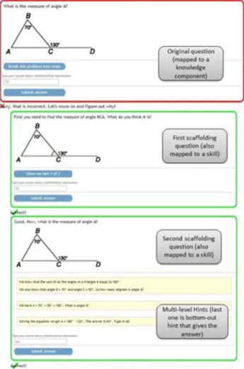
For this work, data from the ASSISTments intelligent tutoring system (Feng, Heffernan & Koedinger, 2009) was used. ASSISTments is a web-based ITS used primarily by middle- and high-school students. In the 2012-2013 school year, it is being used by 40,000 students, mostly in the Northeastern USA, around once a week. While using ASSISTments, students are assessed based on their performance within the system, which is reported back to teachers. Additionally, students are assisted while working through problem sets in three main ways: hint messages, which progress from high-level hints to a “bottom-out hint” containing the answer to the problem; feedback given when the student gives incorrect answers; and scaffolding, where the system breaks a problem down into sub-problems. An example of a student working through a problem in ASSISTments is shown in Figure 1.

Figure 1: Example of a student working through a problem in ASSISTments, from top to bottom. The student first answers the question incorrectly, resulting in feedback. The problem is then scaffolded, and the student answers the first

(14)

7

scaffolding question correctly. Finally, the student clicks through all the hint messages of the second scaffolding question, reaching the “bottom-out hint,” which contains the answer the student types in to solve the problem.

Within this study, data previously collected was used in analysis. The data was collected from ASSISTments data logs from September 2004 to May 2005 for 724 students from four central Massachusetts middle schools, consisting of 107,382 problem attempts. This data set was chosen because the affect detector had already been applied to it and it had been used in a previous study (e.g., San Pedro et al, 2013b). Each problem attempt includes the ID of the student that made the attempt, the problem ID, the relevant “skill” being tested by the problem (e.g., multiplication, area, equation-solving, etc.), and the “type” of problem or method of answering the question (e.g., multiple choice, fill-in, etc.). There were 10 different types of problems and 70 skills represented. Additionally, each problem attempt was labeled with a real-valued confidence level between 0 and 1 that boredom was present. Confidences can be interpreted as the detector’s estimate of the probability that the student was bored at a specific time. These values were computed using a real-time boredom detector, discussed in full detail in (San Pedro et al, 2013b); in brief, this detector was developed by synchronizing thousands of field observations of boredom (with inter-rater reliability over 0.6) with log files, and using data mining to infer the human codes. The mean boredom confidence across all problem attempts was 0.2469 (SD = 0.1293). Confidences were used instead of binary predictions of boredom, in order to leverage the detector’s ability to distinguish cases it is unsure of – for instance, claiming that a case with 51% certainty is identical to a case with 100% certainty, but is fundamentally different from a case with 49% certainty, throws out considerable information and increases the noise in the data set.

B. Modeling Method

To determine whether boredom can be modeled better as a state or trait construct, we fit linear regression models to the data to predict the confidence of the boredom detector. One model is trained using only the problem ID from each problem attempt as a predictor, while the other uses only the student ID from each problem attempt as a predictor. The state theory hypothesizes that the difference between problems will predict much of the variance in student boredom, while the trait theory hypothesizes that the difference between students will predict much of the variance in boredom. The R2 and Bayesian Information Criterion (BiC’; Raftery, 1995) values of the predictions made by these models can then be used to assess which construct is a better predictor of boredom. Additionally, a third model is fit with both problem ID and student ID as predictors. Similar procedures to that described above have been performed for gaming the system in order to assess whether it is better viewed as a state or trait construct (Baker, 2007; Gong et al, 2010; Muldner et al, 2011). Baker’s analysis found that lessons predicted gaming better than students, which was contradicted by the findings of the other two groups (Gong et al, 2010; Muldner et al, 2011); further unpublished analysis conducted by two of these research groups working together suggests that this may be due to differences in the operational definition of gaming used in the different studies. In line with Baker’s method, we use IDs rather than the average confidence of

(15)

8

affect detector results; however, we analyze state-level prediction at the problem-level as in (Muldner et al, 2011), rather than analyzing at a coarser grain-size.

Finally, a proxy for fatigue is computed and added to the data. In this study, the proxy for fatigue is operationalized as the number of minutes that passed since the student last took a break of a certain number of minutes. We hypothesize that fatigue will be a successful predictor due to previous findings of relationships between fatigue and boredom (Harris, 2000; Larson & Richards, 1991) and the relationship between boredom and off-task behavior, in which off-task behavior appears to relieve boredom (Baker et al, 2011). We hypothesize that the longer a student goes without an opportunity to relieve their boredom, the higher their boredom will be. A number of linear regression models are built using only this fatigue statistic for different time durations that constitute a break. The best of these fatigue attributes is then combined with predictors from the other models described above and tested.

III. Analyses A. State vs. Trait

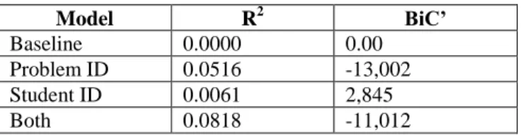
The first research goal was to determine whether state (problems) or trait (students) was a better predictor of boredom. For this analysis, two linear regression models were fit: one that used only problem ID as a predictor, and one that only used student ID. The target attribute for both was the detector’s real-valued confidence that boredom was present. These models were evaluated using two measures: R2, and the Bayesian Information Criterion (BiC’; Raftery, 1995), which calculates the degree to which a model’s predictions are better than what would be expected solely from the number of parameters used. Lower values of BiC’ are better, and a difference of six or more between the BiC’ values of two models is considered equivalent to being statistically significant at the p < 0.05 level (Raftery, 1995). The R2 values were computed using five-fold cross-validation, where the folds were stratified both by problem ID and student ID. The same folds were used for all models, which were built using Matlab’s LinearModel class. The BiC’ values were computed over the entire dataset. The results are shown in Table 1.

Table 1: Model fitting results for state vs. trait. R2_{calculated using five-fold cross-validation, BiC’ calculated over the}

entire dataset Model R2 BiC’ Baseline 0.0000 0.00 Problem ID 0.0516 -13,002 Student ID 0.0061 2,845 Both 0.0818 -11,012

As Table 1 shows, the model based only on problem IDs is significantly more predictive than that based only on student IDs, suggesting that the incidence of boredom is more dependent on the problem being attempted rather than on the student attempting it. Additionally, the student model does worse than the Baseline model (which predicted the mode of boredom confidences, 0.1273,

(16)

9

for all problem attempts) judging by its large positive BiC’ value. A third model that used both student IDs and problem IDs as predictors achieved a higher R2 value, but did worse for the number of parameters it used compared with the model that only used problem IDs, based on their respective BiC’ values.

B. Fatigue

When predicting boredom, it may be helpful to include other factors, such as the current state of the student. One key aspect of the student is whether the student is fatigued. To test this hypothesis, a proxy for the construct of fatigue was added to each problem attempt in the dataset. Fatigue was calculated in two ways, producing models we refer to as MFatigue and PFatigue. MFatigue was calculated as the number of minutes that had passed since the student had taken a break of a certain number of minutes. For example, the attribute “MFatigue(60)” (M stands for minutes) is defined as the number of minutes that have elapsed since the student in question last took a break of 60 minutes or more.

PFatigue was calculated as the number of problems completed by the student since last having a break of a certain number of minutes. We hypothesized that the monotony, and therefore boredom, that the students experienced would increase with the number of problems they completed. For example, the attribute “PFatigue (60)” is defined as the number of problems a given student has completed since last having a break of 60 minutes or more.

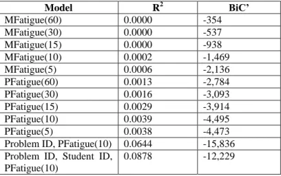
A number of linear regression models were built using each fatigue statistic for different amounts of minutes that constituted a break. This was done since it was uncertain how long of a break was necessary to “reset” a student’s level of fatigue. The results were computed using five-fold cross-validation with the same five folds used for the state and trait models. The results are shown in Table 2.

Table 2: Model fitting results for fatigue. Models including both fatigue and other factors given at bottom.

Model R2 BiC’ MFatigue(60) 0.0000 -354 MFatigue(30) 0.0000 -537 MFatigue(15) 0.0000 -938 MFatigue(10) 0.0002 -1,469 MFatigue(5) 0.0006 -2,136 PFatigue(60) 0.0013 -2,784 PFatigue(30) 0.0016 -3,093 PFatigue(15) 0.0029 -3,914 PFatigue(10) 0.0039 -4,495 PFatigue(5) 0.0038 -4,473

Problem ID, PFatigue(10) 0.0644 -15,836 Problem ID, Student ID,

PFatigue(10)

(17)

10

Both the problem-based and the minute-based fatigue models were better than the baseline model and the student/trait model. However, the problem-based fatigue models were much more predictive than their minute-based counterparts. Using 5 or 10 minutes as the duration of break needed to reset the student’s fatigue produced the best models for predicting boredom from fatigue. The best combination of problem IDs with a fatigue attribute used a break of 10 minutes for resetting fatigue, and significantly improved upon the model that only predicted boredom from the problem ID. This combined (problem ID, fatigue) model was the most predictive model found in these analyses, with a difference in BiC’ of almost 3,000 from the next best model (problem ID). Similarly, adding PFatigue(10) to the (problem ID, student ID) model also improved performance, though this model’s performance still fell short of the problem ID model (or the problem ID, PFatigue(10) model).

Having found that our hypothesis about fatigue being a strong predictor of boredom was correct, we next set out to determine if our hypothesis about higher fatigue leading to higher boredom was correct. However, it turned out that “fatigue” was instead negatively correlated with boredom; e.g., the longer it had been since the student took a break, the less bored they were. Examining the linear regression models based on fatigue revealed that fatigue had a negative coefficient, and correlation analysis showed that all calculations of fatigue were negatively correlated with boredom. The strongest of these correlations was for PFatigue(10), where r = -0.20. It should be noted this correlation was calculated over the entire dataset, and therefore does not correspond to the cross-validated R2 value reported for the PFatigue(10) linear regression model in Table 2. C. Type and Skill

Since problems were found to be more predictive than students, we focused on state explanations of boredom for the remainder of our analyses. Additionally, it has been found that boredom is associated with the difficulty of tasks within achievement settings (Pekrun et al, 2010; San Pedro et al, 2013b). Therefore, as a preliminary analysis of which specific problem features cause boredom in ASSISTments, the association between the type and skill of problems, as defined above, and the level of boredom experienced on them was studied.

Linear regression models were tested using type and skill, using five-fold cross-validation and the same folds used for all previous models. As was done for problems and students, separate models were fit for type and skill, and a third model combining the two was also fit. The results are shown in Table 3.

Table 3: Model fitting results for type and skill

Model R2 BiC’

Type 0.0039 -4,290

Skill 0.0131 -7,063

Type and Skill 0.0184 -8,530

(18)

11

Both the skill and type models outperformed the student ID model, but performed more poorly than the problem ID model. In general, the results also indicate that the skill of a problem is more predictive than its type. Combining type and skill into one model further improved performance, but still not to the same level as the problem ID model. Additionally, PFatigue(10) proved useful again as adding it to the (type, skill) model significantly improved performance – but again, still not to the level of the problem model. Therefore, skill and type seem important, but it appears there are other important problem features missing from this analysis due to the differences in predictive power of the type and skill model and the problem ID model. A full study of which problem features lead to boredom (cf. Doddannara et al, 2013) is warranted.

IV. Discussion and Future Work

Contrary to previous work (Larson & Richards, 1991), we found that state (individual problems) was more predictive of boredom than trait (individual students) in an intelligent tutoring system, ASSISTments. Two possible explanations for this are the different methodologies employed by the two studies, and the different contexts in which boredom was studied.

First, boredom in this work is measured by an unobtrusive computational detector, whereas the prior study measured it using questionnaires and interviews (Larson & Richards, 1991); these differences in measurement may change the results in multiple ways. For instance, potential differences in student comfort and attitudes in self-reporting their boredom could drive the appearance of a student-level effect within self-report methodologies. Second, this work studied boredom at the individual problem level within an intelligent tutoring system, whereas the prior study looked at boredom at a much higher level. The prior study looked at variations in boredom across different subjects like mathematics and English; across different activities within the school environment (such as listening to a teacher or student, reading, and taking a test or quiz); and across school, home, and public environments (Larson & Richards, 1991).

Since it appears that boredom is caused more by individual problems than by students, at least in the context of ASSISTments, future work should focus on identifying which features of problems are the most responsible for boredom. Identifying such features will help inform the design of problems in the future to reduce boredom, increase learning rates, and reduce long-term disengagement.

In this work, two features of problems were considered: the skill (multiplication, equation-solving, etc.) and the type of problems (multiple choice, fill-in, etc.). The linear regression model that considers these features together achieves a paltry R2 of 0.0184, leaving a significant portion

of the R2 achieved by the problem ID model (0.0516) unexplained. Future work should explore

what other properties of problems contribute to boredom.

The level of knowledge a student possesses in a given skill has been shown to explain some of the variance in boredom, though one study found boredom to be higher among highly skilled students (Larson & Richards, 1991) while a set of five other studies have found the opposite relationship

(19)

12

(Pekrun et al, 2010). Therefore, the relative difficulty of a problem or skill may help predict boredom in an intelligent tutoring system context. Looking beyond the aforementioned high-level problem features, a process for determining relevant features similar to what was done by Doddannara et al. (2013) may be relevant and useful for following up the results seen here. Additionally, we found that modeling a proxy for student “fatigue” can add predictive power to the problem model. The best operationalization of fatigue was the number of problems completed since the student last had a break of 10 minutes or more. However, somewhat surprisingly, this measure we constructed as a proxy for fatigue was negatively correlated with boredom. From the results and above analysis, it appears there is merit in considering attributes like fatigue that are not specific to problems (i.e., not uniquely identified by problem ID), but that describe the “session” (what a student completes in a single sequence of activity) or the student’s current state. It may be worth considering further attributes of this nature, such as how many times the student has seen the current skill, or how the current problem relates to previous problems in the problem set in terms of their other attributes, such as difficulty, skill or type.

In this work, we have shown that (at least within the ASSISTments ITS) boredom is better explained by problems (state) than students (trait). We did initial research into the specific components of state boredom within an ITS by fitting models to attributes of problems (type, skill) and the session (fatigue), both of which performed better than the baseline model at predicting boredom. Future work should consider additional factors such as problem difficulty, student knowledge (which is specific to individual students but changes dramatically over time, and which is more consistent with state than trait), and the amount of previous practice the student has had, among other state features.

Another valuable area of work is to follow up this work with replications in other online learning environments, and using alternate operationalizations of boredom (as in the follow-ups to (Baker, 2007) by Gong et al. (2010) and Muldner et al. (2011) for gaming). By better understanding the factors that influence whether a student becomes bored while using an ITS, we may be able to develop more emotionally-sensitive learning systems that lead to better learning and higher long-term engagement.

(20)

13

Chapter 3: Determining the effect of monotony on boredom in intelligent

tutoring systems

I. Introduction

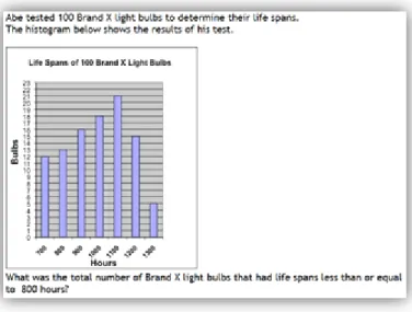
The purpose of this study is to determine whether monotonous content in an intelligent tutoring system (ITS) causes student boredom. We define monotonous content as problem sets whose problems are very similar to each other in terms of the skill(s) and steps required to complete them, the cover story used to give context to the problem, images used, and any other details that could make them seemingly indistinguishable from each other as a student works through them. A retrospective analysis using machine-learned affect detectors (San Pedro et al, 2013b) conducted over ASSISTments (Feng, Heffernan & Koedinger, 2009) data from the 2009-10 school year showed that one of the most boring skill builders (a problem set where a student must answer three consecutive questions correctly to complete) in the system was one that helped students learn how to read histograms. This problem set had the same cover story for every question (light bulb lifespans), used four similar histogram images, and asked two similar types of questions about the data: how many light bulbs had lifespans less than or equal to a certain number of hours, and how many had lifespans greater than or equal to a certain number of hours. An example of one of these questions is shown in Figure 2. We believe the high degree of similarity among the problems of this problem set, or its monotony, is the reason it was among one of the most boring skill builders in ASSISTments.

Figure 2: Example of a “light bulb” question in ASSISTments. II. Methods

To test this hypothesis, we conducted a randomized controlled trial in ASSISTments. We designed a problem set focused on histograms that, when assigned to students, randomly placed

(21)

14

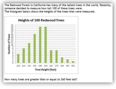
them into one of two types of conditions: control, where students saw questions that were very similar to each other, and experimental, where students saw a mixture of different types of questions. In order to make the experimental condition possible, we created additional histogram questions that were similar in terms of the questions asked and the hint messages provided on the original questions, but that had different cover stories and used different images. Including the original questions, this gave us four unique cover stories, with four histogram images associated with each of them. Figure 3 shows an example of a problem whose cover story is about the heights of trees in the Redwood Forest. The other two cover stories added to the problem set were about the running speeds of cheetahs, and the distances that students were able to throw softballs in gym class.

Figure 3: Example of a histogram question whose cover story is about heights of trees in California’s Redwood Forest. While only one mixed condition is necessary, several control conditions are necessary to isolate monotony as the reason we see any potential effects. It could be the case that some questions are more engaging than others due to the nature of their cover stories, which could lead students who see those questions in the mixed condition to be less bored than those who only see one of the less engaging questions. This would lead to the erroneous conclusion that reducing monotony reduces boredom, when instead the observed effect was actually caused by students seeing engaging questions. To combat this, we had one control condition per cover story, where students in a given control condition only saw questions with the cover story that corresponds to that condition. Having a separate control condition for each cover story allows us to see if any of the questions are inherently more engaging than the others, helping us to separate that from any effect that reducing monotony may have on boredom.

Finally, we noticed that a more recent version of the 2009-10 histograms problem set still had only one cover story, but also only used one image instead of four. Therefore, we added a fifth control condition where students only see light bulb questions that all share the same image. This

(22)

15

gave us six conditions total, where half of the students were randomly assigned to one of the five control conditions, and the other half were assigned to the experimental condition. The diagram in Figure 4 shows what students assigned to different conditions may have seen in terms of cover stories and images.

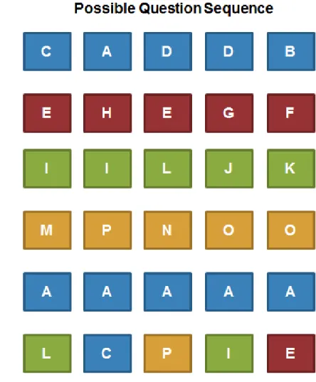
Figure 4: Possible questions sequences for students in each condition.

In Figure 4, the name of the condition appears in the left column, while a possible sequence of questions a student in that condition may see appears to the right, where each question is represented by a colored box containing a letter. The color of the box indicates the cover story of the question, and the letter inside the box indicates the histogram image used. The first five conditions in the figure are control conditions as described above, which means their questions all have the same cover story (and therefore, the same color in the figure). The fifth condition has the same cover story as the first, but uses only one unique image instead of four (therefore, the letters inside the boxes must all be the same). Finally, the last condition, which is the experimental “Mixed” condition, may include questions with any of the four cover stories and

(23)

16

any of the four associated histogram images. Therefore, its boxes may have different colors and letters from each other.

Since the questions in our problem set can be interpreted as histograms or bar graphs, we made two copies of the problem set: one for sixth grade (when histograms are covered, according to the Common Core State Standards) and one for third grade (when bar graphs are covered). Therefore, it is possible we could see an interaction effect between grade level and monotony regarding boredom.

In order to assess the impact of monotony on boredom, we applied the affect detectors developed for ASSISTments in (San Pedro et al, 2013b). These include detectors for boredom, concentration, confusion and frustration. Therefore, in addition to boredom, we also analyzed the data to determine if monotony had any effect on any of the other three affective states.

We ran the experiment in January and February 2014, during which time 125 students worked on the problem set. However, we only wanted to analyze students who had never completed the original histograms problem set before. This left us with 66 students: 30 had been assigned to one of the control conditions, and 36 to the experimental condition.

III. Results

We conducted three types of analyses: overall, where we simply looked at the average incidence of each affective state in the control and experimental groups, previous performance, where we split the analysis based on students’ previous performance in ASSISTments, and previous affect, where we split the analysis based on students’ previous average inferred level of each affective state. Due to the low number of students that participated in the experiment (who had not previously completed a histograms problem set in ASSISTments), we did not analyze the control conditions separately, nor did we analyze the third grade and sixth grade problem sets separately. For each of the analyses reported here, all differences in means were tested with two-tailed t tests to compute p-values. Storey’s (2002) false discovery rate procedure was then used to compute q-values from these p-q-values. None of the computed q-q-values were significant, though a few of the original p-values were marginally significant.

Overall

None of the differences in overall means between the control and experimental groups were significant at the 0.05 level, though the difference between average frustration in the control and experimental conditions is marginally significant before the FDR adjustment (p = 0.0640, t(64) = -1.8848). These means are reported in Table 4.

Table 4: Average confidence of each affective state for each condition, first averaged within each student, then averaged across all students.

(24)

17

Control 0.2752 0.7669 0.2661 0.3737

Experimental 0.2778 0.7669 0.2838 0.3998

Split by Previous Performance

For each class that participated, we split the students in each class into two groups: low-performance and high-low-performance, based on class rank. We did this by computing the percentage of questions that each student answered correctly in ASSISTments during the entire school year, not counting the current experiment, and then assigned the top 50% of the students in each class to the high-performance group, and the bottom 50% of each class to the low-performance group.

Once we split the students into these two groups, we performed the same analysis we did above, but did so for each group of students separately. The results are shown in Table 5.

Table 5: Average confidence of each affective state split by condition and previous performance.

Boredom Concentration Confusion Frustration

Low High Low High Low High Low High

Control 0.2542 0.3067 0.7669 0.7669 0.2482 0.2930 0.3757 0.3706

Experimental 0.2161 0.3330 0.7669 0.7669 0.3609 0.2148 0.4098 0.3908

None of these differences were significant. There was just one marginally significant difference, which was between low- and high-knowledge students in the experimental condition in terms of boredom before the FDR adjustment (p = 0.0602, t(34) = -1.9439).

Split by Previous Affect

Similar to the previous analysis, in this analysis, students in each class were split into two groups by class rank, but this time by how often they exhibited each of the four affective states. Therefore, there were four different orderings, one for each state. The results are shown in Table 6.

Table 6: Average confidence of each affective state split by condition and previous performance.

Boredom Concentration Confusion Frustration

Low High Low High Low High Low High

Control 0.2333 0.3475 0.7669 0.7669 0.2707 0.2601 0.3679 0.3812

(25)

18

None of the differences here were significant either, only the difference in frustration across conditions for those with a history of low frustration was marginally significant before the FDR adjustment (p = 0.0869, t(32) = -1.7662).

IV. Discussion and Future Work

Although it appears that there may have been some effects with marginal reliability, these are most likely statistical artifacts according to Storey’s FDR adjustment (Storey, 2002). Therefore, it is difficult to make any conclusive claims about the outcome of the study.

It is possible that some or all of the observed marginal effects (before the FDR adjustment) are real, but not detectable with the small number of students in the study. For example, it is possible that seeing multiple cover stories is more frustrating than seeing just one, possibly because it forces the students to read each new problem statement rather than just being able to get into a rhythm and extract the important information quickly, which is easier if the problems all look the same. Additionally, seeing multiple cover stories could widen the gap in boredom between low- and high-achieving students. Low-achieving students are more likely not to know the new material and actually need to learn from it, and therefore seeing the new skill applied in multiple contexts as they are learning it may be more engaging. On the other hand, high-achieving students may already know the new skill and just want to get through it, making variable irrelevant cover story details a distraction to them. However, all of this is conjecture without a larger study to confirm it.

Another possible reason for there being no reliable effects is that there was a “ceiling effect” – the vast majority of the students in both conditions finished the problem set in three problems, which is the minimum (students needed to answer three consecutive questions correctly on the same day to complete the assignment). Therefore, students may simply have not had to spend enough time in the problem set for there to be a detectable effect on their affective states.

Therefore, the next logical step would be to run a larger study with more difficult skills to determine whether monotony affects students’ affective states. More difficult skills will help avoid the “ceiling effect,” and more students will make effects more detectable, if in fact there are any.

(26)

19

Chapter 4: Using tabling methods and ensembling to improve student

performance prediction

In the field of educational data mining, there are competing methods for predicting student performance. One involves building complex models, such as Bayesian networks with Knowledge Tracing (KT), or using logistic regression with Performance Factors Analysis (PFA). However, Wang and Heffernan showed that a raw data approach can be applied successfully to educational data mining with their results from what they called the Assistance Model (AM), which takes the number of attempts and hints required to answer the previous question correctly into account, which KT and PFA ignore. We extend their work by introducing a general framework for using raw data to predict student performance, and explore a new way of making predictions within this framework, called the Assistance Progress Model (APM). APM makes predictions based on the relationship between the assistance used on the two previous problems. KT, AM and APM are evaluated and compared to one another, as are multiple methods of ensembling them together. Finally, we discuss the importance of reporting multiple accuracy measures when evaluating student models.

This chapter was published at the following venue:

Hawkins, W., Heffernan, N.T., Wang, Y., Baker, R.S.J.d. (2013) Extending the Assistance Model: Analyzing the Use of Assistance over Time. Proceedings of the 6th International Conference on Educational Data Mining, Memphis, TN, pp. 59-66.

I. Introduction

Understanding and modeling student behavior is important for intelligent tutoring systems (ITS) to provide assistance to students and help them learn. For nearly two decades, Knowledge Tracing (KT) (Corbett & Anderson, 1995) and various extensions to it (Pardos & Heffernan, 2010a; Wang & Heffernan, 2012; Xu & Mostow, 2012) have been used to model student knowledge as a latent using Bayesian networks, as well as to predict student performance. Other models used to predict student performance include Performance Factors Analysis (PFA) (Pavlik, Cen & Koedinger, 2009) and Item Response Theory (Johns, Mahadevan & Woolf, 2006). However, these models do not take assistance information into account. In most systems, questions in which hints are requested are marked as wrong, and students are usually required to answer a question correctly before moving on to the next one. Therefore, the number of hints and attempts used by a student to answer a question correctly is likely valuable information.

Previous work has shown that using assistance information helps predict scores on the Massachusetts Comprehensive Assessment Systems math test (Feng & Heffernan, 2010), can help predict learning gains (Arroyo et al, 2010), and can be more predictive than binary performance (Wang, Heffernan & Beck, 2010). Recently, it has been shown that using simple probabilities derived from the data based on the amount of assistance used, an approach called the Assistance Model (AM), can improve predictions of performance when ensembled with KT (Wang & Heffernan, 2011).

(27)

20

This work continues research in the area of using assistance information to help predict performance in three ways:

1. Specifying a framework for building “tabling methods” from the data, a generalization of

AM

2. Experimenting with a new model within this framework called the Assistance Progress Model (APM), which makes predictions based on the relationship between the assistance used on the previous two problems

3. Experimenting with new ways of ensembling these models to achieve better predictions

Additionally, the importance of reporting multiple accuracy measures when evaluating student models is discussed, as well as why three of the most commonly reported measures (mean absolute error (MAE), root mean squared error (RMSE) and area under the ROC curve (AUC)) do not always agree on which model makes the most accurate predictions.

Section II describes the tutoring system and dataset used. Section III describes the methodology: the models and ensembling methods used, the tabling method framework, and the procedure for evaluating the models. Section IV presents the results, followed by discussion and possible directions for future work in Section V.

II. Data

The data used here was the same used in (Wang & Heffernan, 2011), which introduced AM. This

dataset comes from ASSISTments, a freely available web-based tutoring system for 4th through

10th grade mathematics.

While working on a problem within ASSISTments, a student can receive assistance in two ways: by requesting a hint, or by entering an incorrect answer, as shown in Figure 5.

(28)

21

Figure 5: Examples of assistance within ASSISTments (from Wang and Heffernan, 2011)

The dataset comes from four Mastery Learning classes conducted in 2009, where students worked on problem sets until achieving some criterion, usually specified as answering three questions in a row correctly. The questions in these problem sets were generated randomly from templates, with the difficulty of each question assumed to be the same as all other questions generated from the same template. No problem selection algorithm was used to select the next question.

Two hundred 12-14 year old 8th grade students participated in these classes, generating 17,776 problem logs from 93 problem sets. However, due to the nature of the models studied in this paper, data from two of these students could not be used since these two students never answered more than one question within the same problem set.

Since two of the models cannot be used to predict performance on the first question of a problem set, as they rely on assistance usage on previous problems, these models were not trained or evaluated on the first question answered by a student on a given problem set. This reduced the dataset for these models to 12,099 problem logs. KT models were still trained using the entire dataset, but only evaluated on the 12,099 logs they had in common with the other models.

III. Methods

This section begins by giving an overview of KT, then introduces a framework for building data-driven student models called “tabling methods,” and describes two such methods: AM and APM. Next, the approaches used to ensemble these individual models together are briefly discussed. Finally, the procedure and measures used to evaluate all models are discussed.

(29)

22 Knowledge Tracing

KT is a well-studied student model introduced in (Corbett & Anderson, 1995) that keeps track over time of the probability that a student has mastered a given skill, given their past performance as evidence. The probability that a skill for a given student is in the “known” (vs. the “unknown”) state can then be used to predict future performance.

Constructing KT models involves learning four parameters:

1. Initial Knowledge (L0) – the probability the student has mastered the skill before

attempting the first question

2. Learn Rate (T) – the probability the student will have mastered the skill after attempting a given question if they have not mastered the skill already, independent of performance 3. Guess Rate (G) – the probability the student will answer correctly despite not having

mastered the skill

4. Slip Rate (S) – the probability the student will answer incorrectly despite having mastered the skill

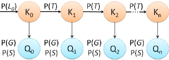
KT models can be represented as static, “unrolled” Bayesian networks, as shown in Figure 6. The level of knowledge Km at time step m influences performance on question Qm. Initial

knowledge influences K0, while knowledge at time step m-1 influences knowledge at time step m

for m > 0. The learned T, G and S parameters are the same across all practice opportunities, meaning that the conditional probability tables (CPTs) for all nodes Km where m > 0 have the

same values, and the CPTs for all Q nodes have the same values.

Figure 6: Static Bayesian network representation of Knowledge Tracing

In this work, the Bayes Net Toolbox for Matlab (Murphy, 2001) is used to create separate KT models for each problem set. The parameters for each model are learned using Expectation-Maximization, with initial values of 0.3 for L0, 0.09 for T, 0.1 for G and 0.09 for S.

Tabling Methods

In previous work (Wang & Heffernan, 2011), a data-driven approach called AM was used to predict performance based on the number of attempts and hints used on the previous problem. This was done by creating a table of probabilities of the student answering the next question correctly on the first attempt without any hints, indexed by the number of attempts and hints used

(30)

23

on the previous problem. These probabilities were computed simply by computing the percentage of questions answered correctly on the first attempt with no hints, parameterized by the number of attempts and hints used on the previous problem.

Then, unseen test data was predicted by using the number of attempts and hints used on the previous problem to do a table lookup. The corresponding probability of getting the next question correct in the table was assigned as the prediction.

In this work, we present a generalization of this approach that serves as a framework for data-driven approaches for student modeling. The general procedure is as follows:

1. Create a table based on one or more attributes of the training data.

2. Compute the probability of answering a question correctly for each combination of values

of the attributes selected in Step 1, and insert these probabilities into the proper cells in the table.

3. For each previously unseen test case, do a table lookup based on the attributes of the test case to obtain the probability (over the training data) of the student answering the question correctly.

4. Assign the retrieved probability as the prediction for the test case.

The attributes selected in Step 1 can be anything available or computable from the data, such as the number of hints and attempts used on the previous problem as AM does, or the correctness of the previous problem, the time taken, the type of skill, etc. These attributes could also represent which bin an instance falls into, where bins are constructed by splitting up students and/or problems based on some criteria.

Cells may need to be added to the table when values for one or more of the attributes are not available, depending on the nature of the attributes. If there are not enough data points for certain cells, it may help to simply combine them with others. Finally, depending on the nature of the selected attributes and the data, it may be useful to split certain cells based on some criterion. In this work, two data-driven approaches that follow this framework are explored: the Assistance Model, as described by Heffernan and Wang and further described below, and the Assistance Progress Model (APM), which constructs a table based on the relationships between hints and attempts used on the previous two problems.

Assistance Model

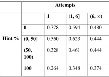
As described previously, AM consists of a table of probabilities of a student answering a question correctly based on the number of attempts and the percentage of available hints used on the previous problem of the same skill. Attempts are broken into three bins: 1, (1, 6] and (6, ∞),

(31)

24

while the percentage of hints is broken into four: 0, (0, 50], (50, 100) and 100. The AM table constructed from the entire dataset is shown in Table 7.

Table 7: AM table for entire dataset Attempts Hint % 1 (1, 6] (6, ∞) 0 0.778 0.594 0.480 (0, 50] 0.560 0.623 0.444 (50, 100) 0.328 0.461 0.444 100 0.264 0.348 0.374

For instance, according to Table 7, when students answered correctly on the first attempt with no hints, they answered the next question correctly 77.8% of the time. On the other hand, if they required over six attempts and used all of the hints available, they answered the next question correctly only 37.4% of the time.

According to Table 7, when attempts are held constant, the general trend is that as hint usage increases, the probability that the student will answer the next question correctly decreases. This makes sense since hints are more likely to be used by students with lower knowledge of the skill. When hints are held constant, different patterns occur with respect to the number of attempts used. When no hints are used, the probability of answering the next question correctly decreases as the number of attempts increases. This relationship is reversed when all hints are used. Finally, if just some of the hints are used, making a few attempts (between 2 and 6, inclusive) helps more than making one attempt, but making many attempts (> 6) decreases the probability of answering the next question correctly.

The pattern for no hints can be explained as more attempts required being indicative of lower student knowledge. For all hints being used, more attempts may indicate the student is attempting to learn rather than just requesting hints until the answer is given to them. Using some of the hints suggests the student has not mastered the skill, but has some knowledge of it and is attempting to learn. The relationship between making one attempt and making a few attempts can be explained by the more attempts the student makes, the more they learn, to a point. The use of excessive amounts of attempts probably indicates the student is not learning, despite using some of the hints.