Precision-mapping and statistical validation of quantitative trait loci by machine learning

Precision-mapping and statistical validation of quantitative trait loci

by machine learning

Justin Bedo

_{, Peter Wenzl}

_{, Adam Kowalczyk}

_{and Andrzej Kilian*}

Address: 1_{Life Sciences, NICTA and Department of Electrical and Electronic Engineering, The University of Melbourne, Parkville, Victoria 3010,} Australia, 2_{Diversity Arrays P/L, 1 Wilf Crane Cr. (Yarralumla), Canberra, ACT 2600, Australia and} 3_{The Research School of Information Sciences} and Engineering, The Australian National University, Canberra, Australia

Email: Justin Bedo - [email protected]; Peter Wenzl - [email protected]; Adam Kowalczyk - [email protected]; Andrzej Kilian* - [email protected]

* Corresponding author

Abstract

Background: We introduce a QTL-mapping algorithm based on Statistical Machine Learning (SML) that is conceptually quite different to existing methods as there is a strong focus on generalisation ability. Our approach combines ridge regression, recursive feature elimination, and estimation of generalisation performance and marker effects using bootstrap resampling. Model performance and marker effects are determined using independent testing samples (individuals), thus providing better estimates. We compare the performance of SML against Composite Interval Mapping (CIM), Bayesian Interval Mapping (BIM) and single Marker Regression (MR) on synthetic datasets and a multi-trait and multi-environment dataset of the progeny for a cross between two barley cultivars.

Results: In an analysis of the synthetic datasets, SML accurately predicted the number of QTL underlying a trait while BIM tended to underestimate the number of QTL. The QTL identified by SML for the barley dataset broadly coincided with known QTL locations. SML reported approximately half of the QTL reported by either CIM or MR, not unexpected given that neither CIM nor MR incorporates independent testing. The latter makes these two methods susceptible to producing overly optimistic estimates of QTL effects, as we demonstrate for MR. The QTL resolution (peak definition) afforded by SML was consistently superior to MR, CIM and BIM, with QTL detection power similar to BIM. The precision of SML was underscored by repeatedly

identifying, at ≤ 1-cM precision, three QTL for four partially related traits (heading date, plant

height, lodging and yield). The set of QTL obtained using a 'raw' and a 'curated' version of the same genotypic dataset were more similar to each other for SML than for CIM or MR.

Conclusion: The SML algorithm produces better estimates of QTL effects because it eliminates the optimistic bias in the predictive performance of other QTL methods. It produces narrower peaks than other methods (except BIM) and hence identifies QTL with greater precision. It is more robust to genotyping and linkage mapping errors, and identifies markers linked to QTL in the absence of a genetic map.

Published: 2 May 2008

BMC Genetics 2008, 9:35 doi:10.1186/1471-2156-9-35

Received: 21 October 2007 Accepted: 2 May 2008 This article is available from: http://www.biomedcentral.com/1471-2156/9/35

© 2008 Bedo et al; licensee BioMed Central Ltd.

This is an Open Access article distributed under the terms of the Creative Commons Attribution License (http://creativecommons.org/licenses/by/2.0), which permits unrestricted use, distribution, and reproduction in any medium, provided the original work is properly cited.

Background

The notion that DNA polymorphism explains the pheno-typic diversity of living organisms has been the driving force behind the Human Genome Project and widespread investment in plant and animal genomics. Over the last 30 years, many examples of causal effects on phenotypes arising from DNA sequence variation have been reported. Finding associations between DNA variation and pheno-types is straightforward for 'simple' traits that are inher-ited in a Mendelian fashion as monogenic characters. Yet, most of the economically important phenotypic variation (e.g. crop yield and its components) is inherited through a number of Quantitative Trait Loci (QTL) with different magnitudes of effect and complex interactions among themselves and with the environment [1].

QTL can be identified through their genetic linkage with molecular markers. In a typical experiment, the progeny of an experimental population are simultaneously ana-lysed for their genetic makeup (molecular markers) and one or more phenotypic traits of interest. The marker data are used to build a genetic map, which is a pre-requisite for the majority of QTL-detection methods [2,3]. The sim-plest method to identify markers linked to QTL is single Marker Regression (MR), which fits a linear model to each marker using the trait data. Simple Interval Mapping (SIM) disentangles QTL effects from the confounding effect of linkage distance between markers and QTL by regressing phenotypic data on the genotypic information for marker intervals rather than the markers themselves [4]. QTL are detected by 'stepping' through the whole genome to generate a profile of the proportion of pheno-typic variance explained or the logarithm-of-odds ratio (LOD score) in favour of a QTL.

The Composite Interval Mapping (CIM) approach refines the SIM algorithm by incorporating background markers as cofactors into a multiple regression model [5]. In this way, variation due to other QTL can be partly accounted for. The CIM approach was further extended by using mul-tiple marker intervals to fit multi-QTL models to the trait data and selecting the 'best' model with a stepwise for-ward and backfor-ward selection procedure (Multiple Interval Mapping; MIM) [6]. Other approaches such as Bayesian Interval Mapping (BIM) [7] approach the problem by applying Bayesian inference over the whole genome using priors designed to produce sparse models.

Here we explore a conceptually quite different QTL-map-ping approach that focuses on generalisation ability. The approach is based on Statistical Machine Learning (SML) and differs from other methods in that it estimates the generalisation performance of a QTL model by splitting the data into independent training and testing subsets that are used for model induction and evaluation,

respec-tively (Figure 1). Resampling data into training and test-ing subsets is quite common in microarray analyses, particularly in the context of cancer genomics [8,9]. Our QTL detection method determines the contribution of each marker to the model performance during the recursive feature elimination (RFE) procedure. First, a lin-ear model containing every marker is fitted to the pheno-type. The model is then reduced in size by recursively eliminating the least useful markers and refitting the model until only a single marker is left, which is similar to recursive feature elimination support vector machines [10,11]. We assign the change in variance explained after each elimination (measured on the test set) to the marker that was removed. The entire process is then repeated numerous times to derive an unbiased bootstrap estimate of the predictive power of each marker. To generate a QTL profile across the genome, the contributions of genetically linked markers within a sliding map window are added. We compare the performance of the SML algorithm with the performance of two conventional QTL-mapping methods (MR, CIM) and the more recently developed BIM. For this purpose, we re-analyse a well-known multi-trait and multi-environment dataset for a population of doubled haploid (DH) lines derived from the F₁ of a cross between cultivars Steptoe and Morex, and study some syn-thetic datasets.

Results and Discussion

Treatment of multi-environment data

In QTL mapping, we are primarily interested in quantify-ing the influence of genotypic variation on phenotypes. In practice, this is confounded by environmental variation to differing extents depending on the trait. In this paper, we limit our approach to mapping the genotypic component of the traits. The interaction between QTL and environ-ments (QTL × E), an important element influencing phe-notypic variation of many quantitative characters, will be addressed in a separate paper.

In order to precisely measure the genotypic component we use data collected on genetically identical Steptoe/ Morex DH lines grown in multiple environments. We standardise the phenotypes within each environment to a mean of 0 and a standard deviation of 1, and then calcu-late the mean (per phenotype and genotype) across all environments. The scaling within environments aligns the distributions, and the averaging provides an estimate of the common underlying signal. The resulting increase in QTL detection power for a whole-genome SML model based on 548 markers is demonstrated in Figure 2; incor-porating information from multiple environments pro-vides an increase in the variance explained for all traits.

The benefit from increasing the number of environments differs between traits. This is not surprising as more envi-ronments will provide a better estimate of the genotypic variation, thus traits that are heavily influenced by the environment are expected to benefit more from the inclu-sion of more environments. The latter is seen clearly for lodging, α-amylase, and plant height where the inclusion of more environments produces a substantial increase in performance over a single environment. We can therefore use the degree of increase in variance explained as a crude measure of environmental "susceptibility" or, conversely, heritability of the trait. For example, heading time appeared to be less influenced by environmental factors (2-fold increase in variance explained) than plant height (3.5-fold increase) and the degree of lodging (5.5-fold increase). The performance improvement due to the

inclusion of multiple environments is, of course, accom-panied by a decrease in the fraction of the total (multi-environment) variance that remains after averaging the scaled phenotypes across environments (Table 1), and thus the latter can also be used as an estimate of environ-mental susceptibility.

Model size and genetic complexity of traits

The SML algorithm combines Recursive Feature (marker) Elimination (RFE) with ridge regression and bootstrap-ping (see Methods). It starts with a whole-genome model and progressively eliminates individual markers from the model. When the algorithm starts removing markers with predictive value, the predictive variance explained starts dropping. The number of markers in the smallest model that explains a close-to-maximum fraction of the variance

System dataflow diagram Figure 1

System dataflow diagram. Dataflow diagram (DFD) depicting the QTL analysis. Rectangles with round corners indicate processes, other rectangles indicate data stores, and lines indicate data flow. The left figure shows the top-level DFD, the right shows further detail of the 'SML analysis' process.

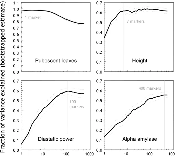
(the 'optimal model') can therefore be used as an indica-tor of the genetic complexity of a trait.

Figure 3 displays the performance of models of varying size obtained through recursive feature elimination. The size of the 'optimal model' varied considerably among different traits. For pubescent leaves, it is evident that the optimal model contains one marker only – indeed the locus determining the character (mPub). All additional markers actually decrease performance as they only add noise rather than information. This effect was also

observed for other traits such as yield (not shown). Plant height is an example of a trait that can be accurately mod-elled with a small number of markers, thus suggesting a relatively low genetic complexity. Diastatic power and α -amylase, by contrast, are traits that appear to be geneti-cally quite complex. For example to accurately model dia-static power, 100 markers are required, while 400 markers are required for α-amylase. These large numbers suggest that the genetic signal is spread out throughout the genome, and that many markers influence (with small individual effects) the phenotypic outcome.

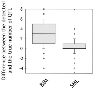
To verify the accuracy of estimating the number of QTL, we performed simulation experiments using a group of 100 artificial datasets. These datasets were simultaneously analysed by Bayesian Interval Mapping (BIM) [12,13] for the purpose of benchmarking our method. Each dataset contained 1-10 QTL positioned randomly at markers evenly spaced at 1 cM intervals across ten chromosomes of 100 cM length. As shown in Figure 4, the median differ-ence in the number of detected QTL for SML is zero, with a low variance. This result demonstrates that the genetic complexity of traits can be estimated very precisely from the performance curves given by the SML method. By con-trast, BIM tends to underestimate the number of QTL.

Multiple environments Figure 2

Multiple environments. Effect of including phenotypic data from multiple environments before modelling. Along the x-axis is

the number of environments used in the pre-processing of phenotypic data, and the y-axis is the fraction of variance explained.

For each number of environments, all possible permutations of the available environments were tested. Each permutation was evaluated by a 50-permutation bootstrap of a whole-genome model fitted using ridge regression. Dotted lines are 95% confi-dence intervals for the mean derived using the t-test.

Number of environments sampled for SML 1 2 3 4 5 6 7 8 9 10 Fraction of va ri ance expl ained (boo tstrapped esti mate) 0.0 0.1 0.2 0.3 0.4 0.5 0.6 0.7 1 2 3 4 5 6 7 8 9 10 1 2 3 4 5 6 7 8 9 10 11 12 13 14 15 16 17 18 Yield Heading Height Alpha amylase Protein content Malting quality Lodging Diastatic power

Table 1: Percentage of total phenotypic variance remaining after averaging scaled phenotypes across environments.a

Trait Variance (%) α-Amylase 52.2 Diastatic power 74.1 Malt extract 54.0 Heading date 70.4 Plant height 64.2 Lodging 40.3

Grain protein content 45.6

Yield 22.4

a _{The number of environments was 6 for lodging; 9 for} α_-amylase,

diastatic power, malt extract, and grain protein; and 16 for the remaining traits.

Statistical validation of QTL through bootstrapping

An important estimation technique used in our method is bootstrap resampling. Bootstrap resampling involves cre-ating a subset of the data for training, and using the remainder for testing (see Methods). In this way, inde-pendent data are reserved for testing the model derived from the training data. This approach produces less biased

estimates of the generalisation error (the predictive per-formance of a model on data unseen during training), and hence a better estimate of the true effect of a putative QTL [14].

Figure 5 illustrates the bias that can occur when not using independent DH lines for testing the predictive power of

Reduction of model size Figure 3

Reduction of model size. Performance of models of varying size (number of markers) for four traits: pubescent leaves, plant

height, diastatic power, and α-amylase. The x-axis is the number of features (markers), and the y-axis is the fraction of variance

explained, estimated using the zero bootstrap. Vertical grey lines indicate the optimal operating points. Dotted lines are 95% confidence intervals derived using the t-test.

Fraction

o

f

var

iance

exp

lained (b

oo

tstrappe

d

est

imat

e)

Number of markers incorporated into SML model

1 _{10 100 1000} 0.0 0.1 0.2 0.3 0.4 0.5 0.6 0.7 1 _{10 100 1000} 0.0 0.1 0.2 0.3 0.4 0.5 0.6 0.7 1 marker 7 markers 100 markers 400 markers

Pubescent leaves

Height

Alpha amylase

Diastatic power

a QTL model. We used MR to detect the top QTL and esti-mate its predictive performance, both using bootstrap resampling and resubstitution (i.e. deriving an estimate based on the whole dataset). For the bootstrap analysis, 200 iterations were used. Each iteration involved detect-ing the top QTL usdetect-ing MR and traindetect-ing a sdetect-ingle QTL linear model on the training data, then estimating the variance explained on the independent test data (the withheld DH lines). In the figure, the red crosses and box plots show the results obtained with resubstitution and bootstrap resam-pling, respectively. For each trait except pubescence leaves, the resubstitution estimate is overly optimistic, sitting outside the upper quartile of the bootstrap estimate. This result illustrates that resubstitution estimates of QTL effects are inherently biased upward. As a consequence, bootstrap resampling reduces the detection of spurious QTL; QTL deemed important on the training set by chance will not reflect the same importance when measured on the test data. Other authors have explored resampling techniques such as cross-validation in the context of QTL detection and evaluation [14], and the biases that arise when not using resampling methods have been well dem-onstrated. Hence the use of bootstrap resampling in the SML procedure should facilitate more robust QTL detec-tion.

QTL identified compared to other methods

Real data

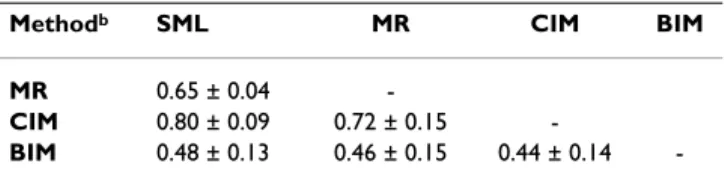
To further benchmark SML against other QTL mapping methods, we identified QTL for nine traits using SML, sin-gle Marker Regression (MR), Composite Interval Mapping (CIM) and BIM. In the case of CIM we used 20 markers at > 10 cM distance from the investigated interval to adjust for the genome background. For BIM, the default values specified in the R/qtlbim package were used for the priors and sampling parameters. Table 2 shows the average degree of correlation of the genome profiles of variance explained (the QTL effects) among the various methods. SML and CIM produced the most correlated results (Pear-son's correlation coefficient r = 0.80). This is despite the fact that SML uses marker information only, while CIM requires the additional information of a genetic map. The BIM profiles were less correlated with the profiles gener-ated by other methods on average.

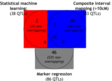
We next counted and compared the QTL reported by SML, MR and CIM at a significance level of p < 0.05 (Figure 6). BIM was not included in this detailed comparison as it is difficult to match the frequentist null-hypothesis rejection thresholds with the Bayes factors used with BIM. SML reported slightly less than half the number of QTL than MR and CIM, presumably because the bootstrap-valida-tion step eliminated spurious QTL (see previous secbootstrap-valida-tion); MR, for example, reported five spurious peaks for pubes-cent leaves, a trait known to be encoded by a single Men-delian trait (Additional File 1). Perhaps not surprisingly, about half of the QTL detected by either MR or CIM could not be cross-validated by a second method. By contrast, 95% of the QTL identified by SML were also detected by MR and/or CIM (Figure 6). These results suggest that QTL detected by SML are more robust and hence more likely to be 'biologically significant'.

There was a large overlap between QTL identified in this study and previous studies of the same DH population [15-18]. SML identified well-known major QTL for α -amylase (chromosomes 2 H, 7 H), diastatic power (1 H, 4 H, 7 H), grain protein content (2 H, 4 H, 5 H), malt extract (2 H, 4 H, 7 H), heading date (2 H), height (2 H, 3 H), lodging (2 H, 3 H, 4 H) and yield (3 H) (Additional File 1) [15-17].

Figure 7 displays the profiles generated using several methods on the heading date, height, lodging and yield traits. The yield QTL on chromosome 3 H at a cumulative map position of 431 cM indeed coincided closely with the main lodging QTL (431 cM) and one of the plant-height QTL (432 cM). Lodging is expected to affect yield, yet the yield QTL profile produced by SML was identical, irrespec-tive of whether or not environments where lodging was reported were included in the analysis (data not shown).

Accuracy of genetic complexity estimates Figure 4

Accuracy of genetic complexity estimates. Compari-son of an analysis of 100 synthetic datasets with BIM and SML. The y-axis shows the difference between the true and estimated number of QTL.

Diffe

ren

c

e

betw

ee

n th

e d

e

tect

ed

and the true

n

umb

er of QTL

BI

M

_SML

Hayes and colleagues suggested that the positive allele for the yield QTL on chromosome 3 H coincided with low lodging and height-QTL alleles from the opposite parent [15]. These previous observations are clearly reinforced by our results and appear to point to a locus influencing plant height that has independent pleiotropic effects on both lodging and yield as opposed to a causal chain (tall

plants → lodging → reduced yield). Plant height also appeared to affect lodging via another QTL on chromo-somes 2 H (241 cM), which coincided for the two traits. Plant height, in turn, appeared to be partly associated with heading date because the main QTL for these two traits coincided precisely (chromosome 2 H; 269 cM). We con-clude that the SML-QTL algorithm confirms and extends previously hypothesised relationships among these traits. Clearly, the resolution of the QTL profiles generated by SML facilitates the genetic dissection of traits into physio-logical or phenophysio-logical components.

Synthetic data

We also compared the genome profiles of variance explained (the QTL effects) derived from the 100 synthetic datasets discussed earlier, in order to benchmark SML against BIM and MR. These methods were selected to rep-resent the two extremes of algorithmic complexity of exist-ing QTL mappexist-ing methods. To summarise these profiles and give an idea of overall performance of each method,

Whole-dataset bias Figure 5

Whole-dataset bias. Demonstration of the optimistic bias that arises when measuring predictive performance on training data. For each trait, the optimal marker was selected using MR, either on the entire dataset (red crosses) or within a 200-per-mutation zero bootstrap environment (box plots).

Alp

ha a

m

yla

se

Di

as

ta

ti

c p

ow

er

M

alting qua

lit

y

Protei

n co

nt

ent

Pubesc

ent

leaves

Hea

di

ng

Heig

ht

Lod

gin

g

_Yi

el

d

Variance explained

(boots

trapped estimate)

whole -dataset estimate

Table 2: Correlation between genome profiles of variance explained obtained with different QTL-mapping methods.a

Methodb _{SML MR CIM BIM}

MR 0.65 ± 0.04

-CIM 0.80 ± 0.09 0.72 ± 0.15

-BIM 0.48 ± 0.13 0.46 ± 0.15 0.44 ± 0.14

-a _{The values given are means ± SD across the nine traits investigated}

in this study.

b _{QTL-detection methods were: SML, Statistical Machine Learning;}

MR, single Marker Regression; CIM, Composite Interval Mapping with 20 background markers at > 10 cM distance from the tested interval, and BIM, Bayesian Interval Mapping.

we considered each dataset to be a binary classification problem – for each marker, classify it as a QTL or not a QTL. Such a binary classification can be accomplished by choosing a threshold and classifying markers exceeding this threshold as linked to QTL. However, as the threshold affects the trade-off between type-I and type-II errors, we used the Area under the Receiver Operating Characteristic (AROC) [19] to measure the performance. The AROC is an order statistic equal to the probability of correctly ordering pairs from different classes (see "QTL classifica-tion performance" secclassifica-tion in Methods).

Figure 8 summarises this experiment in the form of a box plot. The results demonstrate that MR performs worse than BIM and SML – as expected – with a lower median and large variance. BIM achieved a high median perform-ance, but had a larger variance than SML. Though the BIM median was higher, the difference between the means of SML and BIM was not significant (p = 0.499). We con-clude that both methods are similar with respect to locat-ing QTL.

Finally, we examined a single synthetic dataset comprising of a 2,000 cM-long 'chromosome' that contained 20 ran-domly positioned QTL of random strength. Figure 9 shows the smoothed profiles (5 cM averaging window for BIM and 5 cM summing window for SML) of variance

explained obtained using BIM and SML (See Additional File 2). Here it is clear that SML provides better estimates of QTL strength – non-QTL markers are assigned low var-iance explained and the estimates at QTL markers are not overly optimistic. The lack of a bootstrapping step during which experimental units (plants) are resampled presum-ably accounts for the upward bias of BIM (see also section entitled "Statistical validation of QTL through bootstrap-ping"). One may claim that SML is underestimating the variance, however after applying the suggested 5 cM sum-ming window the estimates are improved.

It is important to emphasize that the amount of variance explained supportable by the data will be less than the theo-retical variance explained shown in red due to small sam-ple size (100 samsam-ples with 2001 features) and noise. Measuring the AROC on both variance explained profiles gives 0.83 for SML and 0.78 for BIM, indicating the SML peaks are better aligned with QTL and more distinct than the BIM peaks.

QTL resolution

The precision with which a QTL can be mapped is impor-tant in the context of marker-assisted selection and gene cloning in particular. Narrow QTL peaks are also impor-tant for distinguishing closely linked QTL (or genes) affecting the trait. Figures 7 and 9 demonstrate that SML consistently generated narrower and better defined QTL signals than MR, CIM and BIM. It should be noted that we used quite aggressive settings for CIM to produce narrow QTL peaks (background markers at > 10 cM) [5]. To eval-uate the precision of SML, we investigated the centromeric region on chromosome 7 H flanked by markers Amy2 (64 cM) and Brz (95.2 cM) (Additional File 3). This region contains several overlapping QTL for malting-quality traits, including malt extract, α-amylase and diastatic power [15,18].

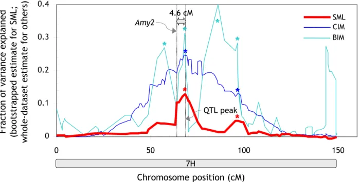
It had been speculated that one of the two α-amylase QTL could be attributed to Amy2, a structural gene encoding low-pI α-amylase [15]. The resolution afforded by conven-tional QTL-mapping methods, however, was insufficient to settle this issue. The CIM analysis in this study also reported a broad peak on chromosome 7 H. The QTL pro-file generated by SML, by contrast, showed two distinct peaks (Figure 10; Additional File 1). One of the two peaks was at 4.6-cM distance from the Amy2 locus (the other was further away). Given that various partially related traits mapped to identical QTL with less than 1-cM precision (Figure 7), a 4.6-cM distance would suggest the structural gene and the QTL are not identical. This result is indeed consistent with a fine-mapping study of this region that identified recombinants between Amy2 and the QTL [18] and hence underscores the high resolution afforded by SML.

Cross-validation of QTL Figure 6

Cross-validation of QTL. Overlaps among QTL detected

by SML, MR and CIM at a p < 0.05 level. QTL in common

between each pair of methods were identified as described in the section entitled 'Comparisons between QTL-detection

methods and map versions' in Methods. The reported

num-bers are the sums across all nine traits investigated in this study. Statistical machine learning: (38 QTLs) Composite interval mapping (>10cM) (83 QTLs) Marker regression (86 QTLs) 7 4 25 11 2 40 46 (53% non-overlapping) (48% non-overlapping) (5% non-overlapping)

Comparison of different QTL methods Figure 7

Comparison of different QTL methods. Genome-wide QTL profiles for four traits generated by SML, MR, CIM and BIM.

A 5 cM averaging window was applied to the BIM profile for plotting. Horizontal dotted lines are p < 0.05 thresholds for SML.

The plots are based on the allele calls and genotypes underlying the 'raw' version of the linkage map (see section entitled

'Genetic-map construction' in Methods).

Heading 0.0 0.1 0.2 0.3 0.4 0.5 0.6 0.7 MR CIM SML p<0.05 threshold (SML) BIM Height 0.0 0.1 0.2 0.3 0.4 Lodging 0.0 0.1 0.2 0.3 0.4 Yield

Genome position (cumulative cM)

0 100 200 300 400 500 600 700 800 900 1000 1100 0.0 0.1 0.2 0.3 0.4 1H 2H 3H 4H 5H 6H 7H

Fraction of variance explain

ed

(bootstrapped estimate for SML; non-bootstrapped estimates for others)

241 cM 269 cM 269 cM 241 cM 432 cM 1036 cM 241 cM 431 cM 431 cM

Conventional methods map QTL with limited precision, particularly if the fraction of the variance explained by a QTL is low [20]. In CIM, the width of QTL peaks can be reduced by using more closely linked markers for genetic-background adjustment. This approach, however, decreases the statistical power of the method [5] and relies on an ad-hoc cM-distance threshold. BIM provides a simi-lar degree of resolution as SML but appears to overesti-mate QTL effects to an even larger extent than CIM, and reports QTL peaks not supported by the other methods (Figure 10).

By contrast, SML generates unbiased QTL models and increases QTL definition by shrinking the size of the mod-els through recursive marker elimination and apportion-ing variance to individual markers based on nested models. Individual markers are evaluated in the context of other markers; so if multiple markers contain a similar

level of information then the (largely) superfluous mark-ers will be removed. The remaining marker(s) will still explain most of the variance, while the variance attributed to the superfluous markers will be small, thus resulting in well-defined QTL peaks.

Robustness to genotyping and linkage-mapping errors

Genotyping errors affect the accuracy of the marker order on a genetic map and hence the performance of QTL-detection methods that require a linkage map. We com-pared the QTL profiles produced with SML, CIM and MR using two different genotypic datasets: the dataset under-lying a 'raw' version of the Steptoe/Morex map (0.4% potential genotyping errors; 97.0% call rate) and the data-set corresponding to a 'curated', re-optimised version of the map (potential genotyping errors removed; 99.6% call rate). Table 3 presents an overview of this comparison. The QTL profiles were highly correlated for MR, less

corre-QTL profile accuracy on simulated data Figure 8

QTL profile accuracy on simulated data. Accuracy of different methods of classifying individual markers as linked to syn-thetic QTL on 100 simulated datasets. Results of genome profiles obtained using BIM, SML, and MR on 100 simulated datasets. The y-axis here is the Area under the Receiver Operating Characteristic (AROC). The 0.5 level indicates random performance and 1 indicates perfect performance.

Area under

the Receiver

Oper

ating

Char

acteristic (AROC)

BIM

_SM

L

M

R

0.0

0.5

0.6

0.7

0.8

0.9

1.0

SML and BIM genome profiles on synthetic data Figure 9

SML and BIM genome profiles on synthetic data. Estimated QTL effects using BIM and SML for a single synthetic 'chro-mosome' of 2,000 cM length with 20 simulated QTL. QTL were positioned randomly with random strength. Red lines indicate true QTL locations, with height denoting strength. BIM profile smoothed using a 5 cM averaging window, and SML profile smoothed using a 5 cM summing window.

SML

Var

iance explained

(bootstrapped estimate)

True

Modelled

BIM

'Chromosome' position (cM)

(non-boot

strapped estimate)

lated for SML and the least correlated for CIM. Despite the high correlated QTL profiles, only 67% of more than 80 QTL identified with MR were consistent between the two map versions. The between-map consistency of the QTL detected with CIM (approximately 80) was even lower (64%).

As a result of the bootstrap-validation step, SML reported less than half of the QTL identified by other methods (see

section entitled Statistical validation of QTL through

boot-strapping above). However, 81% of these QTL were

con-sistent between map versions. In contrast to CIM, the SML method can function independently of a genetic map. We only used the map for smoothing and conveniently plot-ting the results. An erroneous marker order in a linkage map, therefore, affects SML only marginally during the final smoothing/plotting step.

Table 3: Consistency between QTL detected with 'raw' and 'curated' genotypic data.

Total number of QTL detected (p < 0.05)

Methoda _{Correlation between QTL profiles}b _{Raw dataset Curated dataset Overlap}c

SML 0.895 ± 0.085 38 34 29 (81%)

MR 0.998 ± 0.002 86 84 57 (67%)

CIM 0.887 ± 0.128 83 86 57 (67%)

a _{SML, Statistical Machine Learning; MR, single Marker Regression; CIM, Composite Interval Mapping with 20 background markers at > 10 cM}

distance from the tested interval.

b _{QTL profiles are whole-genome plots of the fraction of variance explained vs. genome position similar to those displayed in Figures 6-8. The values}

reported are means ± SD across the nine traits investigated in this study.

c_{The percentage overlap was computed by division by the average number of QTL detected with the two datasets.}

QTL for α-amylase on chromosome 7 H Figure 10

QTL for α-amylase on chromosome 7 H. QTL profiles produced with SML, CIM and BIM. The positions of the structural

α-amylase gene (Amy2) and the maximum of the SML QTL peak are indicated by vertical dotted lines. A 5 cM averaging

win-dow was applied to the BIM profile for plotting. 'Significant peaks' (p < 0.05 for SML and CIM; 2log BF > 2.2 for BIM) are

high-lighted by asterisks. The plot is based on the allele calls and genotypes underlying the 'raw' version of the linkage map (see

section entitled 'Genetic-map construction' in Methods).

0 0.1 0.2 0.3 0.4 0 50 100 150 BIM CIM SML 4.6 cM Amy2

Fraction of variance explained

_{(bootstrapped estimate for SML;}

whole-dataset estimate for others)

Chromosome position (cM)

*

*

*

*

*

*

*

*

estimation of QTL effects. Figure 11 displays a between-map comparison for diastatic power, one of the geneti-cally more complex traits. In the case of SML, the variance explained by QTL was consistent between the two data-sets. CIM was less consistent. For example, map curation reduced the explanatory power of the most important CIM QTL on chromosome 7H from 25% to 10% of vari-ance explained (Figure 11). We conclude from these results that SML is more robust to genotyping and linkage-mapping errors than both MR and CIM.

Interestingly, the quality of the "crude" genotyping data set used in the analysis reported here is lower than that of a typical dataset produced by a standard DArT assay (see the 'Genotypic data' section in Methods) but arguably

(semi)manually scored markers (AFLP or SSR). From this it follows that:

1. 'Standard' QTL mapping approaches (like CIM), when performed on genotyping datasets obtained with gel-based marker technologies, may produce inconsistent marker/trait associations; and

2. The SML approach is likely to perform well in detecting and estimating QTL effects when using marker data with a quality similar to that of a standard DArT assay, with neg-ligible improvement afforded by either replicating DArT assays or employing technically more complex and costly SNP genotyping platform(s).

Robustness to genotyping and linkage-mapping errors Figure 11

Robustness to genotyping and linkage-mapping errors. Effect of map curation on QTL for diastatic power detected by SML and CIM. In the case of CIM, 20 markers at > 10 cM distance from the tested interval were used to adjust for the genetic

background. Statistically significant peaks (p < 0.05) are labelled with asterisks.

(b

ootstr

a

p

p

e

d

e

st

imate

)

V

a

ri

an

ce

e

x

pl

ai

ned

(w

hol

e-data

se

t esti

m

a

te)

SML

CIM (>10cM)

Genome position (cumulative cM)

0 100 200 300 400 500 600 700 800 900 1000 1100 0.0 0.1 0.2

1H

2H

3H

4H

5H

6H

7H

*

*

*

*

*

*

*

*

*

*

*

*

*

* *

* *

_*

*

*

*

*

*

*

*

*

*

*

*

*

*

*

*

*

*

Conclusion

The QTL identified with SML are broadly consistent with those detected by other methods. Yet the SML algorithm offers some advantages over QTL methods such as MR, CIM and BIM. SML produces narrower peaks than MR and CIM and hence identifies QTL with greater precision. BIM generates similarly narrow peaks as SML, but unlike SML seems to underestimate the genetic complexity of traits and overestimate the QTL effects on synthetic data. Because of the use of bootstrap resampling, SML avoids the optimistic bias in predictive performance (% variance explained), which is an inherent feature of other methods. Consequently, SML provides better estimates of the QTL effects supportable by the data, thus reducing the false-discovery rate.

Finally, unlike several other QTL algorithms SML does not require a genetic map. It is therefore applicable to any spe-cies or population. Because of this feature, SML is a poten-tially attractive alternative for association-mapping experiments, an idea that will be explored in a future paper.

Methods

Barley population

Our study is based on existing data for 94 F₁-derived DH plants from a cross between barley cultivars Steptoe and Morex [21-23]. This population has been the subject of extensive phenotyping across a range of environments [22].

Genotypic data

Data source

We used part of the segregation data from a high-quality Steptoe/Morex map with more than 1,000 markers. This map was built from RFLP, DArT and SSR markers [23], and had approximately 0.2% potential genotyping errors. To create a more 'typical' dataset for plant QTL studies reported in the literature (with less markers and a higher error rate), we selected a random subset of 464 markers and added 84 markers with more genotyping errors. The majority of these markers were previously rejected DArT markers with low marker-quality scores [24]. DArT geno-types ('A' for homozygote maternal, 'B' for homozygote paternal) were translated into the original presence/ absence allele calls (0/1) by comparison against the parental alleles. RFLP genotypes were converted into pres-ence/absence allele calls by arbitrarily assigning '1' to the maternal allele.

Allele calls (0/1) were used to identify QTL using SML and MR. Missing allele calls were imputed with 0.5 because the ridge regression algorithm underlying our method works on continuous input values (see section entitled

QTL machine-learning algorithm below). Genotypes (A/B)

were used to identify QTL using the map-based CIM approach. Missing genotypes were replaced with expected genotypes derived from flanking markers after genetic-map construction.

Genetic map construction

For the purpose of displaying SML results and identifying QTL by CIM, we built a genetic map for the dataset of 548 selected markers (351 DArT, 197 RFLP). The marker order was established with RECORD software, and the cM dis-tances between markers were estimated using a multipoint regression algorithm [25,26]. The resulting 'raw' map had a call rate of 97.0% and contained 0.4% potential genotypic errors (Additional File 3). For com-parison, we also generated a 'curated' version of the map. Map curation comprised imputing missing genotypes from neighbouring markers, substituting potential geno-typing errors (LOD_error > 4) [27] with missing data, re-optimising the marker order and collapsing co-segregat-ing markers into 'bins'. The resultco-segregat-ing refined map had 367 bins and a call rate of 99.6% (Additional File 3). We used both the 'raw' and the 'curated' allele calls and genotypes to identify QTL.

Phenotypic data

Data source

The phenotypic data for nine traits, measured in up to 16 different environments, were downloaded from the GrainGenes website [22] (Additional File 4).

Pre-processing of phenotypic data

We introduce a method strongly related to principal com-ponent analysis. Let p_ij be the phenotype measurement for plant i in environment j, n_env, n_mrk, and n_p be the number of environments, markers, and plants respectively. Then the mean and standard deviation of phenotypes within environments are given by

where sj and are the sample standard deviation and

mean of environment j calculated across all plants i ∈

1..np. The scaled phenotypes are then given by

Finally, we can combine the estimates into a single more robust value by calculating the mean across all environ-ments p n p s n p p j p ij i j p ij j i = = − − − −

∑

∑

Note that missing values can be handled during the calcu-lation of s_j and by calculating the mean and standard deviation over available measurements only.

These final values y_i are very similar to results obtained by projecting onto the first principal component. This can be seen by observing that the y_i provide a good linear approx-imation to the full set p_i,j. We verified this on the barley dataset by calculating the principal component projection and measuring the correlation with the values obtained by the above method. The result was a mean correlation coef-ficient of 0.99 across all traits.

Synthetic datasets

Synthetic datasets were created using the R/qtl package [28]. All datasets were simulated backcrosses using an additive model for the phenotype comprising of 100 indi-viduals. Markers were positioned uniformly across the entire genome with no missing values or genotyping errors. The Haldane mapping function was used to con-vert genetic distances to recombination fractions. QTL were distributed randomly at marker positions with uni-form probability. QTL strength (difference between homozygous and heterozygous) was randomly assigned with uniform probability over the interval [-5,5]. Nor-mally distributed noise with mean 0 and variance 1 was added.

QTL machine-learning algorithm

The QTL detection algorithm is based on a few key con-cepts: a linear predictive model, recursive feature elimina-tion, bootstrap resampling for estimation of model performance and marker effects, and generation of QTL profiles by local summation. Figure 1 (left panel) shows a high level overview of the data flow and processing steps involved in generating the QTL profiles. We now detail each concept.

Linear predictive model

Underlying our whole technique is the assumption of lin-ear dependence. We assume that contributions from markers are additive. Let xij be the genotype of plant i at

marker j, and be the vector consisting of all markers from plant i. Under the linear assumption, the estimate of

y_i for plant i is

for plant i, is the associated weight vector, and b is the bias parameter.

The parameters and b are estimated from the training data using the well-known ridge regression algorithm [29,30]. In brief, ridge regression solves the least squares problem

where the first term is the sum of squares, the second term is the regulariser, and λ > 0 is a tuning parameter for adjusting the amount of regularisation. The regulariser encodes a preference for smoother functions by shrinking the weights towards 0 (and also each other), and gives both a unique solution to the ill-posed minimisation problem and increased robustness against noise. For our QTL analyses, we set λ= 1.

Recursive feature elimination

While a model over the entire set of markers is useful for predicting the phenotypic outcome, we wish to determine the key markers contributing to the genetic variation of traits. In other words, we seek a model with K of low car-dinality (i.e. with a low number of elements in the set) that is sufficient for accurate phenotype prediction. This feature (marker) selection is performed by using Recursive Feature Elimination (RFE) to train and evaluate linear models ranging in size from all features to one feature. RFE commences with the full model using all features and then discards the least important feature. This process is recursively applied until a model of desired size is reached (we created models down to one marker). In coupling RFE with ridge regression (RFE-RIDGE), the importance can be estimated from the weights = (β_k). As the model is linear and all markers have the same range, the absolute value |β_k| is an estimate of the importance of the marker

k. The kth _{marker with minimal |}β

k| is deemed the least

important and is discarded. Note that re-optimisation of after each discard is required as the exclusion of a fea-ture will result in a redistribution of weights.

More precisely, let be the model obtained at time step t from applying ridge regression with the set of mark-ers M_t. The initial model at time step t = 1 is fitted with all markers M1 = {1,2,..., m}. At each time step, determine the

y_i n_env p_ij j = −1

∑

∑

∑

∑

least important feature as . The new set of markers for the next time step is then M_t+1 = M_t\{ζ_t}.

Bootstrap resampling

To estimate the performance of models the ε-0 bootstrap method was used [31]. As mentioned previously, this method involves sampling the original dataset with replacement to create a training set, and using all remain-ing un-sampled instances as the independent test set (Fig-ure 1, right panel). The models are then built on the training set, with the test set reserved for the evaluation of model performance. This process was repeated 50 times.

Evaluation of models and estimation of marker contributions

To evaluate the performance of a model we used the frac-tion of variance explained as a criterion. Suppose we have a model ( , b) and we wish to evaluate the variance explained on some test set T. Then, the variance explained is defined as

where . This measure provides an overall

estimation of the predictive performance of a given model.

In addition to evaluating the model, a measure of the con-tribution of individual markers is needed to locate puta-tive QTL. Quantifying these can be done by recasting this problem as a novelty-detection problem: we wish to quantify the amount of additional predictive power pro-vided by each marker given some already selected set of markers. We measure this degree of novelty using the models built with RFE-RIDGE. As RFE-RIDGE produces nested subsets of selected markers, we can attribute the change in variance explained to the marker that was removed between two consecutive models. More

pre-cisely, let be the

sequence of models of decreasing size, i.e.{# j | β_kl = 0} > {# j | β_j(i+1) = 0}, and d_l be the marker eliminated between

ml and ml+1. Then

Δr2 _(d

l) = r2 (ml) - r2 (ml+1)

is a measure of the novelty of a marker with respect to all the remaining markers in the model. We expect that a key QTL marker will be novel in this sense and result in a large change of variance explained when dropped from the model. The average over the bootstrap iterations provides a robust estimate of the importance of each marker to trait prediction. This estimate is referred to as .

Generation of QTL profiles

The information provided by Δr2 _(d

l) is immediately

use-ful; we can examine which markers are found to have sig-nificant contributions. If a linkage map is available, we can use it to create graphs similar to conventional QTL profiles by simply plotting vs. the marker posi-tions. However, the value of a particular genetic location is sometimes 'spread out' among a few highly correlated (genetically close) markers, due to the linkage disequilibrium between the markers and the QTL. This effect can be reduced by smoothing the results based on the positions of markers on a genetic map; for the experi-ments on barley we smoothed the curves by applying a summing window of 5 cM to collect the contributions of genetically close markers. The 5 cM size was chosen because it provides a good balance between resolution and smoothness.

Finally, there are two methods for determining a 95% sig-nificance threshold. We assume the smoothed

were gamma distributed. The gamma assumption is justi-fied as previous literature shows that QTL effects are gamma distributed [32], and 95% thresholds can easily be determined by fitting a gamma distribution. Alternatively, when no smoothing is applied an empirical method can be used to estimate the p-values from the bootstrap repli-cates by applying a standard one-sample t-test.

QTL classification performance

The Area under the Receiver Operating Characteristic (AROC) [19] is a general measure of classification per-formance. We used it to evaluate QTL profiles for simu-lated data where the QTL positions are known. Let s_i be a score (for example the apportioned variance explained produced by the SML) for each marker i, Q be the set of indices of 'QTL markers' and N be the set of indices of 'non-QTL markers.' The AROC is then given by

ξt _k βk t =arg min ( ) G β r b yi f xi b i T yi y i T 2 1 2 2 1 ( , ) min ( ( ; , )) ( ) , G G G β β = − − ∈∑ − ∈∑ ⎛ ⎝ ⎜ ⎜ ⎜ ⎜ ⎞ ⎠ ⎟ ⎟ ⎟⎟ ⎟ y T yi i T = ∈

∑

mated by counting:

Other QTL-mapping methods

Single Marker Regression (MR)

To obtain the fraction of variance explained for individual markers, the Pearson correlation coefficient between the marker and the phenotype was squared. A phenotype per-mutation test of 1,000 iterations was used to derive empir-ical 95% significance thresholds for genome profiles of variance explained [33].

Composite Interval Mapping (CIM)

QTL were also identified by CIM using Cartographer 2.5 software [5,35,36]. The program settings were adjusted to scan the genome at a walk speed of 1 cM. The 20 most important markers, selected by forward stepwise regres-sion outside a 10-cM window on either side of the mark-ers flanking the test site were used to adjust for the genetic background [36]. Experiment-wise 95% significance threshold for likelihood-ratio genome profiles were esti-mated using a permutation test based on shuffling geno-types against phenogeno-types [33,37].

Bayesian Interval Mapping (BIM)

Finally, SML was also benchmarked against BIM [12] using the R package qtlbim [13]. The algorithm was restricted to analysis at marker positions only and not within intervals. Two types of genome profiles were used in experiments – Bayes Factor (BF) profiles for QTL detec-tion, and 'heritability profiles' (i.e. variance explained) for estimating QTL effects. The number of QTL was also esti-mated using Bayes factors.

Comparisons of QTL profiles

The QTL profiles generated by different methods were compared by computing the Pearson correlation coeffi-cient between the genome profiles of variance explained. For the comparison between different map versions (com-prising unequal numbers of markers or bins), the genome scans were first approximated by loess curves based on 1,000 evenly spaced loci.

Statistically significant QTL were identified for each method by recording the cM positions of peak maxima in genome-wide plots of variance explained (p < 0.05). Each contiguous stretch of above-threshold markers was con-sidered to belong to a single QTL peak. Small clusters of

such a stretch of markers (if present) were considered to be part of the shoulder of the same QTL peak. The overlap between the sets of QTL identified using different meth-ods (or map versions) was quantified by counting the instances in which they detected significant QTL within 10-cM of each other.

List of abbreviations

BF, Bayes Factor; BIM, Bayesian Interval Mapping; CIM, composite interval mapping; DArT, diversity arrays tech-nology; DH, doubled haploid; LOD score, logarithm-of-odds ratio in favour of a QTL; LOD_error, logarithm of odds value in favour of genotyping error; MIM, multiple inter-val mapping; MR, single marker regression; QTL, quanti-tative trait locus/loci; RFE, recursive feature elimination; RFE-RIDGE recursive feature elimination – ridge regres-sion; RFLP, restriction fragment length polymorphism; SIM, simple interval mapping; SML, statistical machine-learning; SSR, simple sequence repeat.

Authors' contributions

JB developed and tested the SML algorithm and pheno-type pre-processing procedure, performed the BIM analy-ses and drafted part of the manuscript. PW provided intellectual input during the development and testing of SML algorithms, built the Steptoe/Morex map, performed the CIM analysis, compared the results of the various QTL methods and drafted part of the manuscript. AKo super-vised the development of the SML algorithm and co-edited the manuscript. AKi provided intellectual input during the development and testing of SML algorithms and designed and drafted part of the manuscript. All authors read and approved the final manuscript.

Additional material

∑

Additional file 1

QTL detected with different algorithms (p < 0.05). PDF file containing a list of QTL identified for each combination of QTL-detection method (SML, MR, and CIM) and trait (α-amylase, diastatic power, heading date, plant height, lodging, malt extract, pubescent leaves, grain protein content, and yield).

Click here for file

[http://www.biomedcentral.com/content/supplementary/1471-2156-9-35-S1.pdf]

Additional file 2

Unsmoothed results obtained in the analysis of a synthetic 'chromo-some'. PowerPoint file with two plots containing the unsmoothed results from which the plots in Figure 9 were generated.

Click here for file

[http://www.biomedcentral.com/content/supplementary/1471-2156-9-35-S2.ppt]

Acknowledgements

AKo and JB acknowledge permission of NICTA to publish this paper. NICTA is funded by the Australian Government's Department of Communications, Information Technology and the Arts and the Australian Council through Backing Australia's Ability and the ICT Centre of Excel-lence program. Diversity Arrays Technology Pty Ltd acknowledges financial contribution to this work from the Grains Research and Development Corporation (GRDC).

References

1. Mauricio R: Mapping quantitative trait loci in plants: uses and caveats for evolutionary biology. Nature Rev Genetics 2001, 2:370-381.

2. Asíns MJ: Present and future of quantitative trait locus analy-sis in plant breeding. Plant Breed 2002, 121:281-291.

3. Doerge RW: Mapping and analysis of quantitative trait loci in experimental populations. Nat Rev Genetics 2002, 3:43-52. 4. Lander ES, Botstein D: Mapping Mendelian factors underlying

quantitative traits using RFLP linkage maps. Genetics 1989, 121:185-199.

5. Zeng Z: Precision mapping of quantitative trait loci. Genetics 1994, 136:1457-1468.

6. Kao CH, Zeng ZB, Teasdale RD: Multiple interval mapping for quantitative trait loci. Genetics 1999, 152:1203-1216.

7. Sen S, Churchill GA: A statistical framework for quantitative trait loci mapping. Genetics 2001, 159:371-387.

8. Pomeroy S, Tamayo P, Gaasenbeek M, Sturla L, Angelo M, McLaughlin M, Kim J, Goumnerova L, Black P, Lau C, Allen J, Zagzag D, Olson J, Curran T, Wetmore C, Biegel J, Poggio T, Mukherjee S, Rifkin R, Cal-ifano A, Stolovitzky G, Louis D, Mesirov J, Lander E, Golub T: Pre-diction of central nervous system embryonal tumour outcome based on gene expression. Nature 2002, 415:436-442. 9. Ein-Dor L, Kela I, Getz G, Givol D, Domany E: Outcome signature genes in breast cancer: is there a unique set? Bioinformatics 2005, 21(2):171-178.

10. Guyon I: Gene Selection for Cancer Classification using Sup-port Vector Machines. Machine Learning 2002, 46:389-422. 11. Guyon I: An Introduction to Variable and Feature Selection.

Journal of Machine Learning Research 2003, 3:1156-1182.

12. Yi N, Yandell BS, Churchill GA, Allison DB, Eisen EJ, Pomp D: Baye-sian model selection for genome-wide epistatic quantitative trait loci analysis. Genetics 2005, 170:1333-1344.

13. Yandell BS, Mehta T, Banerjee S, Shriner D, Venkataraman R, Moon JY, Neely WW, Wu H, Smith R, Yi N: R/qtlbim: QTL with Baye-sian Interval Mapping in experimental crosses. Bioinformatics 2007, 23:641-643.

14. Utz H, Melchinger A, Schön C: Bias and sampling error of the estimated proportion of genotypic variance explained by quantitative trait loci determined from experimental data in maize using cross validation and validation with independent samples. Genetics 2000, 154(3):1839-1849.

15. Hayes PM, Liu BH, Knapp SJ, Chen F, Jones B, Blake T, Franckowiak J, Rasmusson D, Sorrells M, Ullrich SE, Wesenberg D, Kleinhofs A: Quantitative trait locus effects and environmental interac-tion in a sample of North American barley germ plasm. Theor Appl Genet 1993, 87:392-401.

16. Hayes PM, Iyamabo I, NABGMP: Summary of QTL effects in the Steptoe × Morex population. Barley Gen Newsl 1994, 23:98-143. 17. Romagosa I, Ullrich SE, Han F, Hayes PM: Use of the additive main effects and multiplicative interaction model in QTL mapping for adaptation in barley. Theor Appl Genet 1996, 93:30-37. 18. Han F, Ullrich SE, Kleinhofs A, Jones BL, Hayes PM, Wesenberg DM:

Fine structure mapping of the barley chromosome 1 centro-mere region containing malt quality QTL. Theor Appl Genet 1997, 95:903-910.

19. Hanley JA, McNeil BJ: The meaning and use of the area under a receiver operating characteristic (ROC) curve. Radiology 1982, 143:29-36.

20. Kearsey MJ, Farquhar AGL: QTL analysis in plants; where are we now? Heredity 1998, 80:137-142.

21. Kleinhofs A, Kilian A, Saghai Maroof M, Byashev RM, Hayes PM, Chen F, Lapitan N, Fenwick A, Balkes TK, Kanazin V, Ananiev E, Dahleen L, Kudrna D, Bollinger J, Knapp SJ, Liu B, Sorrels M, Heun M, Franck-owiak JD, Hoffman D, Skadsen R, Steffenson BJ: A molecular iso-zyme and morphological map of barley (Hordeum vulgare) genome. Theor Appl Genet 1993, 86:705-71.

22. The Steptoe × Morex barley mapping population [http:// wheat.pw.usda.gov/ggpages/SxM]

23. Wenzl P, Li H, Carling J, Zhou M, Raman H, Paul E, Hearnden P, Maier C, Xia L, Caig V, Ovesnα J, Cakir M, Poulsen D, Wang J, Raman R, Smith KP, Muehlbauer GJ, Chalmers K, Kleinhofs A, Huttner E, Kilian A: A high-density consensus map of barley linking DArT markers to SSR, RFLP and STS loci and agricultural traits. BMC Genomics 2006, 7:206.

24. Wenzl P, Carling J, Kudrna D, Jaccoud D, Huttner E, Kleinhofs A, Kil-ian A: Diversity arrays technology (DArT) for whole-genome profiling of barley. Proc Natl Acad Sci USA 2004, 101:9915-9920. 25. Van Os H, Stam P, Visser RGF, van Eck HJ: RECORD: a novel

method for ordering loci on a genetic linkage map. Theor Appl Genet 2005, 112:30-40.

26. Stam P: Construction of integrated genetic linkage maps by means of a new computer package: JoinMap. Plant J 1993, 3:739-744.

27. Lincoln SE, Lander ES: Systematic detection of errors in genetic linkage data. Genomics 1992, 14:604-610.

28. Broman KW, Wu H, Sen S, Churchill GA: R/qtl: QTL mapping in experimental crosses. Bioinformatics 2003, 19:889-890.

29. Hastie T, Tibshirani R, Friedman J: The Elements of Statistical Learning Springer Series in Statistics; 2003.

30. Tikhonov AN: On the stability of inverse problems. Dokl Akad Nauk 1943, 39:195-19.

31. Efron B, Tibshirani R: An Introduction to the Bootstrap Chapman & Hall/ CRC; 1994.

32. Bost B, de Vienne D, Hospital F, Moreau L, Dillmann C: Genetic and nongenetic bases for the L-shaped distribution of quantita-tive trait loci effects. Genetics 2001, 157:1773-1787.

33. Churchill GA, Doerge RW: Empirical threshold values for quan-titative trait mapping. Genetics 1994, 138:963-971.

34. Zeng Z: Theoretical basis for separation of multiple linked gene effects in mapping quantitative trait loci. Proc Natl Acad Sci USA 1993, 90:10972-10976.

35. Basten CJ, Weir BS, Zeng ZB: Zmap – a QTL Cartographer. In Pro-ceedings of the 5th World Congress on Genetics Applied to Livestock Produc-tion: Computing Strategies and SoftwareVolume 22. Edited by: Gavora JS, Chesnais BBJ, Fairfull W, Gibson JP, Kennedy BW, Burnside EB. Guelph, Ontario, Canada: Organizing Committee of the 5th World Congress on Genetics Applied to Livestock Production; 1994:65-66.

36. Basten CJ, Weir BS, Zeng ZB: QTL cartographer: a reference manual and tutorial for QTL mapping Raleigh, NC: Department of Statistics, North Carolina State University; 2005.

37. Doerge RW, Churchill GA: Permutation tests for multiple loci affecting a quantitative character. Genetics 1996, 142:285-294.

Additional file 3

Genotypic data used for QTL analysis. Excel file containing 0/1 allele calls and A/B genotypes (segregation data) for both the 'raw' and the 'curated' Steptoe/Morex genetic map.

Click here for file

[http://www.biomedcentral.com/content/supplementary/1471-2156-9-35-S3.xls]

Additional file 4

Phenotypic data used for QTL analysis. Excel file containing phenotypic data for the nine traits investigated in this study (α-amylase, diastatic power, heading date, plant height, lodging, malt extract, pubescent leaves, grain protein content, and yield). The data is from up to 16 different envi-ronments and includes averages across standardised envienvi-ronments (see section entitled 'Pre-processing of phenotypic data' in Methods). Click here for file

[http://www.biomedcentral.com/content/supplementary/1471-2156-9-35-S4.xls]