Incorporating Detailed Noise Modeling and Multi-Scale
Feature Extraction
Thesis by
Samuel T. Pfister
In Partial Fulfillment of the Requirements for the Degree of
Doctor of Philosophy
California Institute of Technology Pasadena, California
2006
c
2006
Acknowledgements
I wish to extend warm thanks to my adviser, Joel Burdick, for his constant support. Many thanks to Stergios Roumeliotis for early guidance in all subjects central to this work. Thanks to Kristo Kriechbaum and to the rest of the robotics group for their valuable assistance and feedback. Thanks to the Mars Exploration Rover team and the DARPA Grand Challenge team for such wonderful and unique experiences outside of research.
Abstract
Mobile robot localization and mapping in unknown environments is a fundamental require-ment for effective autonomous navigation. Three different approaches to localization and mapping are presented. Each is based on data collected from a robot using a dense range scanner to generate a planar representation of the surrounding environment. This exter-nally sensed range data is then overlayed and correlated to estimate the robot’s position and build a map.
The three approaches differ in the choice of representation of the range data, but all achieve improvements over prior work using detailed sensor modeling and rigorous book-keeping of the modeled uncertainty in the estimation processes. In the first approach, the raw range data points collected from two different positions are individually weighted and aligned to estimate the relative robot displacement. In the second approach, line segment features are extracted from the raw point data and are used as the basis for efficient and robust global map construction and localization. In the third approach, a new multi-scale data representation is introduced. New methods of localization and mapping are developed, taking advantage of this multi-scale representation to achieve significant improvements in computational complexity. A central focus of all three approaches is the determination of accurate and robust solutions to the data association problem, which is critical to the accuracy of any sensor-based localization and mapping method.
Contents
Acknowledgements iii
Abstract iv
1 Introduction 1
1.1 Motivation . . . 1
1.2 Summary of Contributions and Related Work . . . 4
2 Background 9 2.1 Chi-Square Test . . . 9
2.2 Maximum Likelihood . . . 10
2.2.1 A Simple ML Example . . . 11
2.3 Kalman Filter . . . 11
2.4 Hough Transform . . . 13
2.5 Sensors . . . 15
2.5.1 Odometry . . . 15
2.5.2 Range Scanner . . . 18
3 Weighted Scan Matching 22 3.1 Introduction and Overview . . . 22
3.2 The Weighted Range Sensor Matching Problem . . . 26
3.2.1 The Measurement Model . . . 26
3.2.2 A General Covariance Model . . . 28
3.2.3 Displacement Estimation via Maximum Likelihood. . . 29
3.2.4 The Algorithm and Its Initial Conditions . . . 31
3.3 Scan Matching Error/Noise Models . . . 34
3.3.1 Measurement Process Noise . . . 34
3.3.2 Correspondence Error . . . 35
3.3.3 Measurement Bias Effects . . . 37
3.4 Selection of Point Correspondences . . . 39
3.5 Estimating the Incidence Angle . . . 39
3.6 Scan Matching Experiments . . . 41
3.6.1 Robustness and Accuracy Comparisons . . . 41
3.6.2 Multi-Step Runs . . . 48
3.6.3 Comparison of Computational Demands . . . 49
3.7 Weighted Scan Matching Conclusions . . . 50
4 Line-Based Mapping and Localization 54 4.1 Introduction and Overview . . . 54
4.2 Line Feature Definitions . . . 58
4.2.1 Infinite Line Representation . . . 59
4.2.2 Infinite Line Covariance . . . 59
4.2.3 Infinite Line Frame Transformations . . . 60
4.2.4 Infinite Line Center of Rotational Uncertainty . . . 64
4.2.5 Line Segment Representation . . . 65
4.2.6 Line Segment Covariance . . . 67
4.2.7 Line Segment Frame Transformations . . . 67
4.2.8 Line Segment Center of Rotational Uncertainty . . . 69
4.2.9 Subfeature Coordinates . . . 70
4.3 Line Segment Feature Extraction . . . 73
4.3.1 Initial Line Guess . . . 75
4.3.2 Point Grouping . . . 76
4.3.3 Point Noise Modeling . . . 77
4.3.4 Weighted Line Fitting . . . 77
4.3.5 Line Segment Covariance Estimation . . . 82
4.3.6 Subsequent Feature Extraction . . . 82
4.4.1 Hypothesis 1 - Common Infinite Line . . . 86
4.4.2 Hypothesis 2 - Line Segment Overlap . . . 88
4.4.3 Hypothesis 3, 4 - Endpoint Matches . . . 90
4.5 Line Segment Merging . . . 91
4.5.1 Line Segment Merging Examples . . . 93
4.6 Line Segment–Based Kalman Filter . . . 99
4.6.1 Preliminary Definitions . . . 99
4.6.2 Propagation Equations . . . 99
4.6.3 Update Equations . . . 100
4.7 Line Segment–Based SLAM . . . 104
4.7.1 Line Segment–Based SLAM Experiments . . . 104
4.8 Line Segment–Based Mapping and Localization Conclusions . . . 108
5 Multi-Scale Mapping and Localization 109 5.1 Introduction and Overview . . . 109
5.2 Block Feature Definitions . . . 112
5.2.1 Block Feature Representation . . . 113
5.2.2 Block Covariance . . . 113
5.2.3 Block Frame Transformations . . . 115
5.2.4 Block Center of Rotational Uncertainty . . . 116
5.2.5 Subfeature Coordinates . . . 118
5.3 Block Feature Extraction . . . 120
5.3.1 Multi-Scale Hough Transform . . . 120
5.3.2 Endpoint Detection . . . 123
5.3.3 Multiple Feature Detection . . . 124
5.3.4 Extraction Cost Benefits . . . 125
5.4 Block Feature Matching . . . 126
5.4.1 Matching Definitions and Assumptions . . . 128
5.4.2 Block Scale Overlap Hypothesis . . . 128
5.4.3 Block Parameter Match Hypotheses . . . 132
5.4.4 Match Confidence Test . . . 134
5.5.1 Bottom-Up Tree Construction . . . 136
5.5.2 Top-Down Tree Construction . . . 137
5.6 Block Feature Matching Using Scale Trees . . . 137
5.6.1 A Correspondence Example . . . 138
5.7 Localization Using Scale Trees . . . 140
5.7.1 A Localization Example . . . 140
5.8 Block-Based Kalman Filter . . . 142
5.8.1 Preliminary Definitions . . . 142
5.8.2 Propagation Equations . . . 143
5.8.3 Update Equations . . . 143
5.8.4 Block-Based SLAM . . . 146
5.9 The Kidnapped Robot Problem . . . 146
5.9.1 Computational Cost . . . 147
5.10 Multi-Scale Mapping and Localization Conclusions . . . 154
6 Conclusions and Future Work 155 Bibliography 157 A Weighted Scan Matching Calculations 165 A.1 Weighted Translation Solution . . . 165
A.2 Weighted Rotation Solution . . . 165
A.3 Covariance Estimation . . . 168
B Optimal Line Fit Derivation 172 B.1 Covariance of the Virtual Measurements . . . 172
B.2 Center of Rotational Uncertainty Estimation . . . 174
B.3 Determination of the Chi-Square Cost Function . . . 174
B.4 Distance to Line Estimation . . . 174
B.5 Heading to Line Estimation . . . 175
B.5.1 Second-Order Approximation . . . 177
C.2 Heading to Line Estimate Covariance . . . 180 C.2.1 Complete G0
k(0)G
00
k(0) . . . 182
List of Figures
2.1 Infinite polar line L representation. . . 14 2.2 Line representations through a single point in Cartesian space and Hough
space. . . 14 2.3 Line representation through two points in Cartesian space and Hough space. 15 2.4 Geometry of the odometry process. . . 16 2.5 Geometry of the range sensing process. . . 18
3.1 Geometry of the range sensing process. The robot acquires dense range scans in posesiandj. The circles represent robot position, while thex-yaxes denote the robot’s body-fixed reference frames. . . 23 3.2 Representation of the uncertainty of selected range scan points. . . 25 3.3 A) Experiments with initial displacement perturbations between scans taken
at a single pose. B) Close-up of robot pose with results. . . 43 3.4 A) Experiments with initial displacement perturbations between scans taken
at different poses. B) Close-up of pose 2 with results. . . 45 3.5 A) Experiments with initial displacement perturbations in a non-static
envi-ronment. B) Close-up of pose 2 with results. . . 46 3.6 A) Experiments with initial displacement perturbations in a hallway
environ-ment. B) Close-up of pose 2 with results. . . 47 3.7 A) A 109-pose, 32.8-meter loop path. B) Close-Up of final path poses, shown
the covariance estimates of the weighted and unweighted algorithms. . . 52 3.8 A) An 83-pose, 24.2-meter loop path. B) Close-up of final loop poses. . . 53
4.3 Line coordinates with respect to a global frame and a frame at posei. . . 61
4.4 Line coordinates with respect to a global frame and a frame at pose i. The values δρi and δψi represent the poseidisplacement in the “ρ−ψ” frame. . 61
4.5 Projection of pose uncertainty into line L. . . 63
4.6 Infinite line and line covariance representation. ~uP represents the center of rotational uncertainty. . . 65
4.7 Segment S representation. . . 65
4.8 Segment S representation with multiple endpoint pairs. . . 66
4.9 Segment S representation. . . 71
4.10 Segment S and endpoint covariance representation. . . 72
4.11 Segment S and endpoint covariance representation with small σα. . . 73
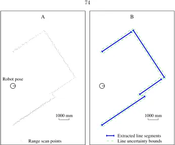
4.12 A) Raw range scan points. B) Extracted line segment features. . . 74
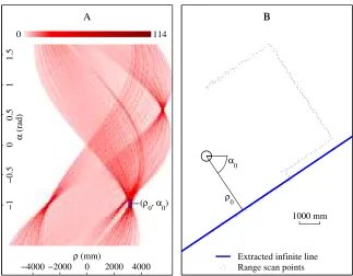
4.13 A) Hough space accumulator. B) Extracted infinite line. . . 76
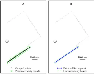
4.14 A) Grouped set of collinear points. B) Optimally fit line. . . 77
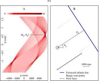
4.15 A) Hough space accumulator. B) Extracted infinite line. . . 83
4.16 A) Grouped set of collinear points. B) Optimally fit line. . . 83
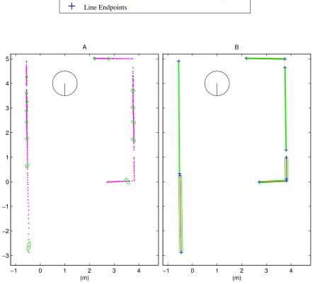
4.17 Range data: A) Raw points and selected point covariances. B) Fit lines and line uncertainties. . . 94
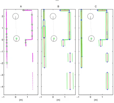
4.18 Range data from two poses: A) Raw points and selected point covariances. B) Fit lines and line covariances. C) Merged lines and line covariances. . . 95
4.19 Range data from eight poses – A) Raw points and selected point covariances. B) Fit lines and line covariances. C) Merged lines and line covariances. . . . 96
4.20 A) Raw points and selected point covariances. B) Fit lines and line covariances. C) Merged lines and line covariances. . . 97
4.21 Line map built with presented SLAM techniques: A) Full raw point data. B) Full line segment map representation. . . 106
4.22 Full line map built with line segment length restriction. . . 107
4.23 Hallway data set: A) Raw data points. B) Full set of fit lines. C) Restricted set of fit lines. . . 107
5.2 Block B representation. . . 113
5.3 Block B and block covariance representation. . . 114
5.4 Block B representation. . . 118
5.5 Block B with subsegment and subpoint features shown. . . 119
5.6 Multi-scale extraction ofρa,ρb: A) Raw scan points B) Hough transform. . . 122
5.7 Fine-scale extraction ofρa,ρb: A) Blockρboundary detection at fine scale. B) Detected infinite block. . . 122
5.8 Coarse-scale extraction of ρa,ρb: A) Block ρ boundary detection at coarse scale. B) Detected infinite block . . . 123
5.9 End extraction at the fine scale . . . 124
5.10 Subsequent block extraction. . . 125
5.11 Example of scale-based difference in the block feature representation of iden-tical point data. . . 127
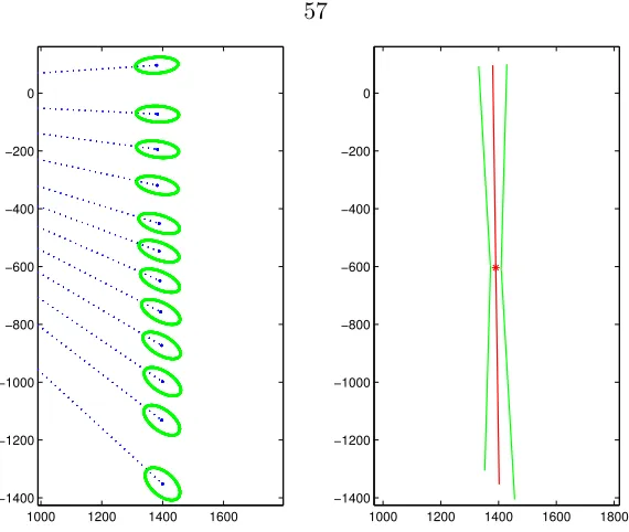
5.12 Multi-scale range scan representation: A) Scale tree for pose 1. B) Finest scale features pose 1. B) Scale tree for pose 2. D) Finest scale features for pose 2. E) Corresponding features from pose 1, pose 2. . . 139
5.13 Multi-scale localization example where the blue circle is pose 1, the red circle is the estimated pose 2, and the black circle is the actual pose 2. A) Initial pose estimates and raw scans. B) Coarse feature fit. C–G) Intermediate pose estimates and feature correspondences at each scale. . . 141
5.14 Kidnapped robot problem data: Multi-scale map and candidate scan repre-sentation at scales of 200 mm, 100 mm, and 50 mm. . . 148
5.15 Kidnapped robot problem data: Multi-scale map representation and candidate scan representation at scales of 25 mm and 12.5 mm. . . 149
5.16 A selection of four hypotheses invalidated at the coarsest scale. . . 150
5.17 A selection of two hypotheses with partial validation at the coarsest scales but invalidated at the 50 mm scale. . . 151
List of Tables
Chapter 1
Introduction
1.1
Motivation
Autonomous robot navigation has long been a goal of researchers for applications rang-ing from military supply convoys, to space exploration, to autonomous highway drivrang-ing. A critical requirement of higher level navigation applications is that the robot has some reasonable knowledge of its current position with respect to a fixed reference frame. For example, in navigation applications that entail motion to a target position, the robot needs an accurate estimate of its current position to plan a path to the goal and to confirm suc-cess. Similarly, for exploration applications, position information can be used and recorded to avoid redundant coverage. The process of position estimation with respect to a fixed reference frame is defined as thelocalization of the robot.
A mobile robot can localize itself using two different classes of on-board sensors: pro-prioceptive sensors and exteroceptive sensors. Propro-prioceptive sensors, such as encoders or inertial measurement units (IMUs), measure the motion of the robot, acquiring data that can be integrated to estimate relative robot displacement. This method of localization is called odometry, or dead reckoning, and when used alone, the integrated error in global position grows without bound over time.
externally sensed data, while using this map to localize. This approach is commonly called simultaneous localization and mapping (SLAM).
This dissertation focuses on localization and mapping using exteroceptive sensors, so the rest of the material is prefaced with a discussion of the several methods used to localize a robot with externally acquired data.
One method of exteroceptive sensor–based localization involves modifying the environ-ment through the placeenviron-ment of easily detectable and identifiable passive or active beacons in known locations, which can then be used as references to triangulate the robot’s position [MM92]. Global positioning system (GPS) based localization falls into this category, as the known global reference map consists of the instantaneous positions of the satellites, and the on-board exteroceptive sensor is the GPS receiver. The simplicity and improving accuracy of GPS-based localization makes it popular for outdoor autonomous applications, but for indoor applications, near tall buildings or high terrain, or in inclement weather, GPS sig-nals can degrade significantly or drop out completely. For truly robust navigation, complete reliance on GPS for localization, even in an outdoor environment, may not be adequate.
Another exteroceptive sensor-based localization method involves comparing the on-board sensor data to a known map representing the geometry of the surrounding envi-ronment. This map can be taken from a blueprint, satellite photos, or other previously built map [BEFW97]. This method is more flexible but more complex than the artificial beacon method, as the correlation of sensed data with the known global map requires a non-trivial solution to the data association problem, while the beacon methods often ben-efit from uniquely identifiable features by design. Though this localization method does not require preconditioning of the environment through beacon placement, it is constrained by the need for prior knowledge of the environment and is therefore not suitable for many applications.
One early mapping method represents the map as an occupancy grid [Elf89]. As obsta-cles are detected, the corresponding cell in the rasterized map is incremented to create a gridded representation of the environment. In contrast, early work by Chatila and Laumond [CL85] introduces a feature-based representation using polyhedra to describe the environ-ment boundaries. Feature-based map representations are often more complex to construct than grid-based maps, as the features need to be extracted from the raw data. Yet these maps are not constrained in their precision like the grid maps, whose precision is limited by choice of cell size. This means that a sparse feature map can hold a much more efficient and accurate representation of the environment than a grid-based counterpart.
Of course, the data representation underlying these feature-based mapping methods can vary drastically, and may depend on the type of external sensor or sensors being used. Some algorithms use cameras as the primary sensor and use features extracted from camera frames as the basis for mapping and localization [AF89, AH93]. Sonar range sensors [Cro89] are commonly used, as are laser radar scanners or ladars [ABL+01]. A variety of feature types
have been developed for extraction from laser range scanner data. These include corners [AMTS04], lines [CT99, AD04], principal components [VK99], or even the raw range data points themselves [LM97b]. Multi-sensory methods also exist which merge and combine information from both range and camera sensors [NTHS99, NW00].
The most successful schemes to estimate map coordinates and robot position have in-volved probabilistic techniques. These schemes implement a SLAM approach where data is collected from an uncertain position and assembled into a map while using that uncertain map to assist in localization. Early work by Smith and Cheeseman [SC86] introduced a probabilistic framework for map building and localization. One current SLAM technique uses an expectation maximization (EM) algorithm to build the map and localize the robot [TFB98]. This algorithm can be used to focus on robust determination of feature correspon-dences [DSTT01]. Another common approach to SLAM uses Kalman filters to estimate the robot position and build the map [RB00a, CMNT99, MDWD02, DDWB00].
There are three primary challenges common to localization and mapping methods, which are the focus of this dissertation:
used to help bound this error, these sensors also provide noisy measurements, which must be addressed.
Problem 2) Data association accuracy: For methods that localize the robot using external sensor information, it is necessary to establish correspondences between data col-lected across different robot positions. If accurate correspondences cannot be determined, then the sensor information is useless for localization. The details of the data association problem differ between the approaches mentioned above, but it is essential for accurate and robust localization and mapping. Data association is made especially difficult in the presence of the sensor noise discussed above.
Problem 3) Robustness to unmodeled errors: In any real-world application there will be events or sensory readings that are outliers when compared to normal operations. For example, wheel slippage due to difficult terrain can cause unmodeled odometry error when integrating wheel rotation. Also a closed door or moved table can introduce discrepancies in external sensor measurements, which are far larger than can be explained by sensor process noise. It is critical that localization methods be robust to, and recover from, these types of unmodeled errors.
The following section summarizes the localization and mapping methods I have de-veloped, and highlights how these methods contribute to the current state of research in robotics.
1.2
Summary of Contributions and Related Work
I developed three exteroceptive sensor-based approaches to localization and mapping pre-sented here. This work assumes planar motion of the robot inSE(2), with no prior knowl-edge of the environment and no communication with beacons such as GPS satellites. The primary sensor used in this work is a dense planar range scanner that returns range point measurements of nearby obstacles. The range scanner is configured to collect data in a plane parallel to the ground surface.
Chapter 3 introduces a weighted scan matching technique that uses dense laser range scan data to compute relative position and orientation displacement of the robot. In the standard unweighted scan matching approach by Lu and Milios [LM97b, LM97a], raw range point data taken from two different robot positions is aligned to generate an updated es-timate of the relative position and orientation displacement. The method first determines a set of point pairs that correspond across the two sets of range point data. The method then calculates the relative position and orientation displacement between the robot posi-tions, which minimizes the sum of the distances between the range point pairs. Because the true data association between points is unknown, an iterative technique is developed, and the point correspondences are recalculated at each iteration-based on the closest point technique. A reasonable initial guess is required so that the method will converge to an accurate estimate
The weighted scan matching algorithm that I developed improves upon the standard approach through rigorous individual noise modeling of the underlying sensing and geom-etry. Modeling for the correspondence error between individual pairs of matching points compensates for the fact that even if two scans are perfectly aligned, the points from dif-ferent scans rarely sample the exact same spot in the environment. Such correspondence error modeling also helps to reduce the effect of mismatched points in the displacement estimate. This results in a more accurate displacement estimate and a more accurate co-variance calculation for the estimation process. Improved coco-variance is especially important for applications where the displacement estimate is fused with measurements from other sensors [RB02].
The results presented in this chapter compare my weighted technique with the standard unweighted approach, showing an improved accuracy in the overall displacement estimate, and a greater robustness to poor initial displacement guesses.
in-troduces significant contributions over prior methods. One contribution of my work is a feature extraction method that takes into account detailed sensor models. Another set of contributions involve techniques for feature correspondence and merging that enable prob-abilistically sound localization and mapping using long line segment features. These long line segment features are constructed by merging together features detected from multiple positions. Unlike in prior work, the features can have a length of many times the maximum range and field of view of the sensor and can span gaps in the environment. Also unlike prior work, this method also enables effective feature correspondence and merging of short line segment features, even lines with no length extracted from an isolated point. This allows for accurate line segment approximation of curved edges and enables effective mapping and localization using contours in the environment that aren’t strictly straight lines.
Like Castellanos and Tardos [CT99, CMNT99], my line segment feature representation is based on the polar form of the line. This polar representation is augmented with end-point position information. To extract the line segment features, I first use the Hough transform [JC98, FLW95, IN99] to initially group collinear range scan points, then com-pute an optimally fit line for the individually weighted points using a maximum likelihood approach.
Some methods describe line segments as a pair of Cartesian endpoints [AF89], but a polar representation enables a more straightforward comparison of the underlying infinite line of different features. This allows for the merging of lines that do not necessarily share common endpoints. Because of this approach, long lines can be assembled over multiple scans. In addition, lines that span gaps in the segments (e.g., a set of lines representing a long wall with open doors) can be merged.
The polar representation unfortunately introduces nonlinear effects caused by the cou-pling between line orientation and position. Castellanos and Tardos compensate for these effects in their localization and mapping methods by only considering lines that have a low uncertainty in orientation. This has the effect of eliminating shorter lines, which tend to have a higher orientation uncertainty. I have developed methods of feature comparison and merging that adjust for the nonlinear effects, and allow for the inclusion of short, even point-like line segments into the localization and mapping process.
a full data representation over the abbreviated feature set of Castellanos and Tardos. Chapter 5 introduces a multi-scale approach to localization and mapping. There are numerous examples of multi-scale feature extraction and matching methods in the vision community [PM90, WRV98, KB01, Low99], but few approaches to mobile robot localization and mapping have taken advantage of these methods. The few attempts at multi-scale data processing for the purpose of mobile robot localization [MDWD02, PR98, TMK04, MT04] focus mostly on noise reduction. They do not attempt the multi-scale feature extraction and correspondence that allows for the significant computational gains demonstrated by my method.
My feature extraction method uses a novel approach to a multi-scale Hough transform, with some similarities to the work of Magli and Olmo [MO01]. The feature itself is a block like feature where the width of the block relates to the scale of extraction. At a very fine scale, a block with near zero width behaves like a line segment feature, as outlined in Chapter 4. The extraction process uses the same sensor noise model as in the previous chapters.
This chapter also introduces a method of establishing feature correspondences that take into account the flexibility of feature description at the coarse scales, while allowing for detailed matching when available. The map representation can be maintained in a tree structure, which allows for significant performance improvements in data correspondence through a tree-based search method.
Also introduced is a multi-scale approach to the “kidnapped robot problem”[Eng94], a problem in which the robot loses knowledge of its position and must recover by relocalizing. This novel multi-scale approach uses a coarse first search across the map for candidate locations, and demonstrates substantial computational benefits for large maps.
The results in this chapter demonstrate use of the multi-scale approach to assist in efficient data correspondence and robust localization. Results for a Kalman filter based SLAM method are presented for multiple scales. The maps built using the SLAM method are used as the reference for tests of the multi-scale approach to the kidnapped robot problem. These multi-scale results do not have a directly comparable method, so most analysis is done in comparison to single-scale feature methods.
Chapter 2
Background
Several common methods used repeatedly in this work are introduced here. First the basics of the chi-square hypothesis are reviewed, which is a critical component of my feature correspondence methods. The maximum likelihood framework for parameter estimation is then introduced, as well as the equations for the extended Kalman filter. Finally the Hough transform based pattern detection method is described, which is the basis of the feature extraction approaches used in Chapters 4 and 5.
2.1
Chi-Square Test
The chi-square test is a common method used to test the goodness of fit of a hypothetical assumption. This test consists of the computation of a chi-square distributed random variable D, corresponding to the measurement and model being tested. The value is then compared with chi-square distribution probability tables to determine the probability that the error seen would be generated by the given model. A threshold can be set such that measurements that are determined to have a low probability of being generated by the model result in the dismissal of the model hypothesis as false.
Given an n-dimensional random variable V and a measurement of this variable ˆV, the assumption to be validated is thatV has a zero mean, normal distribution with a covariance represented by ann×ncovariance matrixPV. The D2 value can be calculated as follows:
D2= (V −Vˆ)T(PV)−1(V −Vˆ). (2.1)
value of D is equivalent to the Mahalanobis distance, which is a unitless distance metric between random variables that is weighted by the relative uncertainty.
The threshold can then be set to a value χ2(P, n), determined by a chi-square distribu-tion table, wherenis the degrees of freedom andP is the probability that the given value ˆV ofV could be generated by the model which has been assumed to be true. In my methods, I set the threshold for a very low probabilityP as I don’t want to throw away a hypothesis that has any reasonable chance of being true. The hypothesis can be invalidated if
D2 > χ2(P, n). (2.2)
It is important to note that while a high value ofD2 does imply a low probability of model accuracy, the converse is not necessarily true. Even in the case where a single measurement exactly matches the model such that D2 = 0, one can only claim with any degree of
certainty that there is not a significant reason to abandon the model. The test alone does not imply that there is a high probability of the model being accurate. The chi-square test is an effective method of eliminating untrue hypotheses, but model validation methods may require an additional, alternate test to detect and reduce instances of wrongly accepting a false hypothesis.
2.2
Maximum Likelihood
The maximum likelihood (ML) method is a framework for parameter estimation given a set of independent measurements of a random variable. In this method, a likelihood function is defined as the product of the likelihood functions of each of nindependent measurements. Given a set of measurements{xˆ1, ...,xˆn}and the parameters to be estimated g=g1, ..., gm
the likelihood function for each measurement can be represented asf(ˆxi, g). The likelihood
function is then
L({xˆk}|g) =f(ˆx1, g)f(ˆx2, g)· · ·f(ˆxn, g). (2.3)
The goal is to determine the value ofgthat maximizes the likelihood functionL. To do this L is differentiated with respect to g and arrive at the following conditions for maximizing the likelihood function:
∂L ∂g1
= 0,· · ·, ∂L ∂gm
It is often beneficial to consider the log of the likelihood function when determining these partial derivatives as the likelihood and log-likelihood have the same extrema.
∂ln(L) ∂g1
= 0,· · · ,∂ln(L) ∂gm
= 0. (2.5)
2.2.1 A Simple ML Example
In a fundamental example of estimating the meanx of a normal distribution and measure-ments {xˆ1, ...,xˆn} each with variance σ, let g =x and compute the likelihood function as
follows:
L({xˆk}|x) =
1 σ√2π
n
eM (2.6)
with
M =
n
X
k=1
−12
xˆ
i−x
σ
2
. (2.7)
Then set the log of the likelihood function equal to zero and solve the partial derivative with respect to x:
∂ln(L({xˆk}|x))
∂x = ∂M
∂x = 0 (2.8)
n
X
k=1
ˆ xi−x
σ
= 0 (2.9)
x= 1 n
n
X
k=1
ˆ
xi. (2.10)
The result is simply that the sample average of the measured values has the maximum likelihood of being the true value ofx. In this work, the same approach is used to address more complex problems of parameter estimation.
2.3
Kalman Filter
state variables and, with each update, the overall mean squared error is minimized. The KF enables a simultaneous localization and mapping (SLAM) approach where the robot builds the map while it uses this dynamically built map to localize.
The fundamental modes of the KF are propagation and update. Propagation occurs as the robot moves with dead reckoning and the pose uncertainty increases according to the propagation process noise. Updates occur when new measurements are made of the environment and this information is incorporated into the filter resulting in a reduction of overall uncertainty.
The primary assumptions for KF optimality are that the system is linear and all random processes have a normal distribution. Due to the nonlinearities introduced by the coupling between the orientation and position measurements, it is common to utilize the extended Kalman filter (EKF) in SLAM implementations, which linearizes the KF equations but relaxes the assumptions of optimality.
In discrete time the evolution of the state vector X is
X(tk) =fk(X(tk−1), u(tk−1), w(tk−1)) (2.11)
where f is a nonlinear function of the state X, the control inputs u and the process noise w. Also consider a measurement zat time tk to be governed by
z(tk) =h(X(tk), v(tk)) (2.12)
wherehis a nonlinear function of the state and measurement process noisev. The resulting filter equations for the propagation step are
ˆ
Xk|k−1=fk( ˆXk−1|k−1)|uk−1,0), (2.13)
Pk|k−1=AkPk−1|k−1ATk +WkQk−1WkT. (2.14)
The estimate ˆXk|k−1 represents the estimate of state X at stepk given all sensed inputs up
to stepk−1, while the values of ˆXk−1|k−1 andPk−1|k−1 represent the state and covariance
zero process noise. Pk|k−1 is the covariance matrix for the state estimate where Ak and
Wk are Jacobian matrices of partial derivatives of f with respect to X and w. The update
equations for the EKF are
Kk=Pk|k−1HkT HkPk|k−1HkT +VkRkVkT
−1
, (2.15)
ˆ
Xk|k= ˆXk|k−1+Kk(zk−h( ˆXk|k−1,0)), (2.16)
Pk|k= (I−KkHk)Pk|k−1, (2.17)
where Hk and Vk are the Jacobian matrices of partial derivatives of h with respect to X
and v calculated at each step k. The state and covariance is represented as ˆXk|k and Pk|k,
respectively, and I is the identity matrix. See [WB95] for an overview of the derivation of the general EKF equations.
2.4
Hough Transform
The Hough transform is a general pattern detection technique commonly used in machine vision applications [DH72]. In this process, each of a set of scan points {~uk}, k = 1, ..., n
is transformed into a discretized curve in the Hough space and accumulated in a discrete rasterized space. This is a voting scheme and the resultant peaks in the Hough space corre-spond to patterns that “agree” with many points. Though the method can be generalized to a wide range of patterns, the focus here is on the implementation as a line detector. Consider an infinite polar line L with a normal distance to the origin, ρ, and a normal angle, α, as shown in Figure 2.1. These parameters ρ and α define the dimensions of the Hough space. Each point in the set of scan points is represented in Cartesian form with the kth point ~u
k= (xk, yk).
Define a Hough spaceH(i, j) as a two-dimensional raster with integer indicesiandjand define the discrete values in each dimension asα(j) andρ(i), respectively. α(j) is discretized in increments of Dα on the range [−π/2, π/2] and ρ(i) is discretized in increments of Dρ
on the range [−ρmax, ρmax] whereρmax is the maximum range value in the point set. The
L
α
ρ
Figure 2.1: Infinite polar line L representation.
a given point, for alli, the positionρik of the line at angle α(i) can be calculated such that
the line would pass through point~uk:
ρik =xkcos(α(i)) +yksin(α(i)). (2.18)
From the value of ρik, determine the indexj such that ρ(j)−Dρ/2 < ρik ≤ρ(j) +Dρ/2.
Then increment the value at Hough space cell H(i, j). After multiple point inputs, the cell in Hough space with the highest incremented value corresponds to the line that has the most contributing points.
−500 0 500 1000 1500 2000 2500 −500
0 500 1000 1500 2000 2500
L1
L2 L3
v1
Y (mm)
X (mm) −2000 −1500 −1000 −500 0 500 1000 1500 2000 2500 −2
−1.5 −1 −0.5 0 0.5 1 1.5 2
L1
L2
L3
v1
α
(radians)
R (mm)
Figure 2.2: Line representations through a single point in Cartesian space and Hough space.
Figure 2.2 shows the Hough transform of a single point v1. On the left, the point and
−500 0 500 1000 1500 2000 0
500 1000
1500 L1
v1
v2
Y (mm)
X (mm) −2000 −1500 −1000 −500 0 500 1000 1500 2000 2500 −2
−1.5 −1 −0.5 0 0.5 1 1.5 2
v1 v2
L1
α
(radians)
R (mm)
Figure 2.3: Line representation through two points in Cartesian space and Hough space.
point and the line determined by the peak of the Hough space at the intersection of the curves.
In Section 4.3.1 the Hough transform is used to group collinear points and to extract the initial guess for the line feature estimation method. In Section 5.3.1 I extend the basic Hough transform to develop a multi-scale feature extraction method.
2.5
Sensors
My motive is to achieve effective mobile robot localization using onboard sensors. There are two basic categories of sensors: proprioceptive and exteroceptive. Proprioceptive sensors (such as encoders or IMUs) sense the motion of a robot and are the basis for odometry or dead reckoning. Exteroceptive sensors (such as laser scanners or cameras) sense the surrounding environment. In this work odometry is used as a proprioceptive sensor, and a dense laser range scan is used as an exteroceptive sensor. In this section I outline the geometric representation of the sensory signal, and the sensor signal uncertainty models that will be referenced in subsequent chapters.
2.5.1 Odometry
g0
Pose g
Pose gi
x
x y
φ
y
φ
i i
i i
i
ij j
j
j
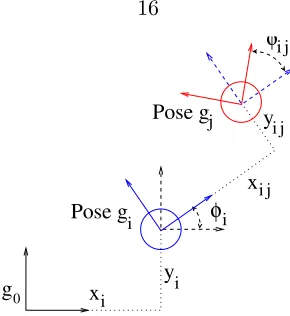
Figure 2.4: Geometry of the odometry process.
relative to a fixed reference frame,g0.
gi =
xi
yi
φi
, (2.19)
wherexi, yi, andφi are described in Figure 2.4. In this representation the robot heading is
denoted to be at angle φi such that the forward direction on the robot corresponds to the
positivex direction.
The odometry system generally estimates relative changes in the robot pose by inte-grating over the internally measured motion of the actuators or the signals of an inertial measurement unit (IMU). If the robot starts at pose i and moves to pose j the resulting local displacement measurement with respect to pose iis denotedgij where
gij =gi−1gj =
xij
yij
φij
(2.20)
as seen in Figure 2.4. The value for gij is a random variable sampled from the robot
odometry system by integrating wheel velocity or from other methods of dead reckoning.
Odometry Noise Model
be defined as
Pgij =
Pxx Pxy Pxφ
Pyx Pyy Pyφ
Pφx Pφy Pφφ
. (2.21)
This is a general covariance matrix. The form of the actual covariance matrix depends on the model of the odometry method being used. A simple, often used, model assumes the noise inx,y, andφis independent for a small displacementgij, in which casePgij simplifies
to
Pgij =
σx2 0 0
0 σy2 0 0 0 σ2
φ
, (2.22)
where the values σ2
x, σy2 and σφ2 represent the variance in x, y and φ, respectively. As this
is represented in the robot local frame, the uncertainty in x corresponds roughly to the uncertainty in the distance moved straight ahead while the uncertainty in y corresponds to the possible side slip of the robot. In practice, over longer distances of integrating the displacement, even small errors in odometry orientation estimation modeled by σ2
φ tend to
have a significant effect on the overall uncertainty of the robot pose due to the integration of lever arm effects.
Given this representation for a local displacement and displacement covariance, the pose transformations that are commonly used in localization and mapping methods are briefly introduced.
Pose Transformations
Given an initial pose gi in the global frame and a measured displacement gij in a frame
local to gi, the current pose estimate gj can be calculated in the global frame as follows:
gj =
xj yj φj = xi yi φi +
cos(φi) −sin(φi) 0
sin(φi) cos(φi) 0
0 0 1
xij yij φij
. (2.23)
be-tween themgij measured with respect to pose gi can be calculated as follows:
gij=
xij yij φij =
cos(−φi) −sin(−φi) 0
sin(−φi) cos(−φi) 0
0 0 1
xi−xj
yi−yj
φi−φj
. (2.24)
Pose Covariance Transformations
Given an initial posegi and covariance of that pose measurementPgi and a local
displace-ment measuredisplace-mentgij with local covariance Pgij, the combined covariance Pgj in the global
frame can be calculated as
Pgj =QPgiQ
T +KP gijK
T, (2.25)
where K =
cos(φi) −sin(φi) 0
sin(φi) cos(φi) 0
0 0 1
(2.26) and Q=
1 0 −ycos(φi)−xsin(φi)
0 1 −ysin(φi) +xcos(φi)
0 0 1
. (2.27)
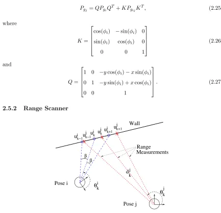
2.5.2 Range Scanner
i uk j k+1 u i uk+1 k uj j k−1 u i uk−1 β β Wall k k Pose j Pose i X X X i MeasurementsRange j θ θ kj d
I assume that at a given pose, the robot measures the range to the boundary of its nearby environment along rays that are separated by a uniform angleβ. As outlined below, I allow for various uncertainties in this range measurement.
Let the set of nscan points from a single pose be denoted by {~uk}, k = 1, . . . , n. The
scan point coordinates are described in the robot’s sensor frame, and thus the expression for thekth scan point has the form
~uk=dk
cosθk
sinθk
, (2.28)
wheredk is the measured distance to the environment’s boundary in the direction denoted
by θk (see Fig. 2.5).
Range Scanner Noise Model
Range sensors can be subject to both random noise effects and bias. For a discussion of bias, see [PKRB02]. Here I briefly review a general model for measurement noise. Recall the representation of scan data in terms of polar coordinates (dk, θk) in Eq. (2.28). Let the
range measurement, dk, be comprised of the “true” range, dk, and an additive noise term,
εd:
ˆ
dk=dk+εd. (2.29)
Also assume that error exists in the measurement of ˆθk, i.e., the actual scan angle differs
(slightly) from the reported or assumed angle. Thus,
ˆ
θk=θk+εθ, (2.30)
where θk is the “true” angle of the kth scan direction, and εθ is again an additive noise
term. Hence the measured point ˆ~uk can be represented as
ˆ
~uk= (dk+εd)
cos(θk+εθ)
sin(θk+εθ)
. (2.31)
assumed to be a zero-mean Gaussian random variable with varianceσ2d and the noise εθ is
assumed to be a zero-mean Gaussian random variable with variance σ2
θ (see, e.g., [AP96]
for justification). If I further assume thatεθ1o (which is a good approximation for most
laser scanners), I can make the assumptions cos(εθ) = 1 and sin(εθ) =εθ. The measured
scan point ˆ~uk can be thought of as consisting of the true component,~uk, and the uncertain
component, δ~uk:
ˆ
~uk=~uk+δ~uk. (2.32)
Expanding Eq. (2.31) and using the relationship δ~uk = ˆ~uk−~uk yields
δ~uk= (dk)εθ
−sinθk
cosθk
+εd
cosθk
sinθk
. (2.33)
Assuming thatεθ andεd are independent, the covariance of the range measurement process
for thekth range point is
Puk 4
=E[δ~uk(δ~uk)T]
= (dk)
2σ2
θ
2
2 sin
2θ
k −sin 2θk
−sin 2θk 2 cos2θk
+ σ
2
d
2
2 cos2θk sin 2θk
sin 2θk 2 sin2θk
.
(2.34)
For practical computation, ˆθk and ˆdk can be used as a good estimates for the quantities θk
and dk.
Nonzero bias assumption.
In the case of a sensor where the zero bias assumption does not sufficiently hold, a bias term~bk is added to Eq. (2.32):
ˆ
~uk =~uk+δ~uk+~bk. (2.35)
The term δ~uk is generally well modeled by a zero-mean Gaussian noise process as outlined
above in Eq. (2.33). The bias~bk is an unknown offset that can be approximated by a term
~ok corrupted by a zero-mean additive Gaussian noise δ~bk [AP96]. The covariance of this
noise component reflects the level of confidence in the value~ok:
In practice, the value of~ok can be determined by statistical analysis of measurement data.
Chapter 3
Weighted Scan Matching
3.1
Introduction and Overview
This chapter introduces an algorithm to estimate a robot’s displacement from a pair of dense range scans. This localization algorithm operates on the raw range scanner data points. In later chapters, I will build on the methods developed here to present localization and mapping algorithms that use higher level features, instead of the simple point range data features used here. Here I focus primarily on the advantages of my “weighted” scan matching algorithm compared to other methods used in the scan matching field.
Scan matching describes the process of correlating the raw range sensor points taken from different poses to obtain an estimate of the displacement between the poses. This novel algorithm takes into account several important physical phenomena that affect range sensing accuracy, and that have been neglected in prior work. The experiments in Section 3.6 show that this algorithm is not only efficient, but more accurate than nonweighted matching methods, such as that of [LM97b]. In addition, by computing the actual covariance of the displacements, the weighted matching algorithm provides the basis for optimal fusion of these estimates with odometric and/or inertial measurements [RB02], and subsequently supports localization and mapping tasks.
To best understand the content of this chapter and its contributions,. I first describe the basic problem, then describe how the solution differs from previous ones, and the generality of my approach.
The robot starts at an initial configuration, g1, and moves through a sequence of
con-figurations, or poses, gi, i = 2, . . . , m. Here gi ∈ SE(2) denotes the robot’s position and
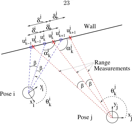
MeasurementsRange i uk j k+1 u i uk+1 j k−1 u i uk−1
αik
θki yj
xj θkj
k u δj− δi−
δ+j
β β Wall x yi i X X α Pose j β β j k Pose i X j
δ+i
Figure 3.1: Geometry of the range sensing process. The robot acquires dense range scans in posesiandj. The circles represent robot position, while thex-yaxes denote the robot’s body-fixed reference frames.
measures the range to the boundary of its nearby environment along rays that are separated by a uniform1 angle, β (see Fig. 3.1). As described below, I allow for various uncertainties
in this range measurement.
Let the set of Cartesian coordinates of the ni scan points taken in the ith robot pose,
be denoted by{~uik}, k = 1, . . . , ni. The scan point coordinates are described in the robot’s
body fixed reference frame. Typically, the Cartesian coordinate of the scan point is derived from range data according to the expression:
~uik =
x
i k
yik
=lki
cosθ
i k
sinθki
, (3.1)
whereli
k is the measured distance to the environment’s boundary along thekth measuring
ray. The measuring ray is oriented in the direction denoted by θi
k, where θik is the angle
made by thekth measuring ray with respect to thex-axis of the body fixed reference frame
(see Fig. 3.1).
The main goal is to accurately estimate the robot’s displacement between poses by matching range data obtained in sequential poses. This displacement estimate can be used as the basis for a form of odometry, or fused with conventional odometry and/or inertial
1
measurements to obtain better relative robot pose estimates. These estimates in turn can support localization and mapping procedures. First, assume that the range scans at poses i and j have a sufficient number of corresponding points to be successfully matched (see Section 3.4). Let{~ui
k, ~u j
k}fork = 1, . . . , nijbe the set of corresponding matched scan point
pairs, where nij is the number of corresponding pairs. From these pairs I first want to
estimate the relative displacement between poses iandj: gij =gi−1gj = (Rij, pij), where
Rij=
cosφij −sinφij
sinφij cosφij
~pij=
xij
yij
, (3.2)
i.e., the displacement between poses i and j is described by a translation (xij, yij) and a
rotation, φij.
Next, I consider the covariance, Pij, of the displacement estimate. This covariance has two uses. First, it reflects the quality of the displacement estimates. Large diagonal elements of the covariance matrix indicate increased uncertainty. Any localization process should be aware of the level of confidence in its computed pose estimates. Second, the covariance is also needed when combining displacement estimates with measurements provided by other sensors. More accurate and realistic estimates of the contributing covariances lead to more accurate overall estimates in a sensor fusion algorithm, such as a Kalman filter.
My approach differs from prior work in that the contribution of each scan point to the final displacement estimate is individually weighted according to that point’s specific uncertainty. The scan point uncertainties are estimated using sensor measurement noise models as well as models of specific geometric issues within the matching process itself. To better understand these issues, examine Figs. 3.1 and 3.2. Fig. 3.1 depicts the situation when a range sensor (e.g., a laser range finder) samples points on a nearby wall. The boundary points sampled in pose i are indicated by circles, and labeled by ~ui
k−1, ~uik, and
~ui
k+1. The nearby boundary points sampled in posej are indicated by X’s and are labeled
by ~ujk−1, ~ujk, and ~ujk+1. Prior range matching methods (e.g., [GG97, VRB02, Cox91]) have made the simplifying assumption that the range scans of different poses sample the environment’s boundary atexactly the same points—i.e., point~ui
kis assumed to be exactly
−6000 −4000 −2000 0 2000 4000
(mm)
Robot Pose
Scan Points Selected Scan Points 100 x Point Covariance (3σ)
Figure 3.2: Representation of the uncertainty of selected range scan points.
As described in Sections 3.3.1 and 3.3.3, the range measurements are corrupted by noise and possibly a bias term that is a function of the range sensing direction, θi
k, and
the sensor beam’s incidence angle, αi
k (Fig. 3.1). Figure 3.2 shows the 95% confidence
level ellipses associated with the covariance estimates (calculated using the methods that I will introduce later) of selected data points from an actual laser range scan. Clearly, the wide variation in uncertainties seen in Fig. 3.2 strongly suggests that not all range data points are of equal precision. Hence, this potentially large variability must be taken into account in the estimation process. While the existence of these uncertainty sources has previously been suggested [BB01, ABL+01, Cox91, Ada00, AP96], my algorithm is the
developing physically based uncertainty models for each individual point and incorporating these models in both the displacement estimation process and the covariance calculation.
The principle behind this approach generally applies to any case of dense range data, such as sonars, infrareds, cameras, radars, etc. The weighted matching formulation and its solution given in Section 3.2 are independent of any sensor specifics. To use the general results, specific models of sensor uncertainty are needed. Some detailed sensor models are developed in Section 3.3. Since some of the assumptions underlying these sensor models are best suited to laser range scanners, the application of the detailed sensor model formulas is best suited to the use of laser scanners in indoor environments, though they can be extended to structured outdoor environments. However, the general approach of Section 3.2 should work for other range sensors and other operating environments with reasonable modifications to the sensor models.
This chapter is structured as follows: Section 3.2 describes a general weighted point feature matching problem and its solution. Section 3.3 develops correspondence and range measurement error models. Sections 3.4 and 3.5 summarize the point pairing selection and sensor incidence angle estimation procedures. Experiments in Section 3.6 demonstrate the algorithm’s accuracy, robustness, and convergence range. Direct comparisons with previous methods (e.g., [LM97b, LM97a]) validate the effectiveness of the approach.
3.2
The Weighted Range Sensor Matching Problem
This section describes a general point feature matching problem and its solution.
3.2.1 The Measurement Model
Let the sets of Cartesian range scan data points acquired in poses i and j be denoted by the{~uˆik}and{~uˆjk}, respectively. These measurements will be imperfect. Let{~uik}and{~ujk} be the “true” Cartesian scan point locations. As discussed in Section 2.5.2 and Eq. (2.35), range scan point measurements can generally be decomposed into the following terms:
ˆ
~uik = ~uik+δ~uik+~bik ˆ
whereδ~ui
k andδ~u j
k represent noise or uncertainty in the range measurement process, while
~bi k and~b
j
k denote the possible range measurement “bias.” These noise and bias terms are
introduced in Section 2.5.2 and discussed in more detail with regard to the weighted sensor matching problem in Section 3.3.3. Let ( ˆ~ui
k,~uˆ j
k) be points that are deemed to correspond in
the range scans at posesiand j. As shown in Fig. 3.1, these points are not necessarily the same physical point, but the closest corresponding points. Accounting for the fact that scan data is measured in a robot-fixed frame, the error between the two corresponding points is
εijk = ˆ~uik−Rij~uˆjk−pij (3.4)
for a given displacement (Rij, pij) between poses. Substituting Eq. (3.3) into Eq.(3.4)
results in
εijk = (~uik−Rij~ujk−pij)
| {z }
(i)
+ (δ~uik−Rijδ~ujk)
| {z }
(ii)
+ (~bik−Rij~bjk)
| {z }
(iii)
. (3.5)
A relative pose estimation algorithm aims to estimate the displacementgij = (Rij, pij) that
suitably minimizes Eq. (3.5) over the set of all correspondences. If the dense range scans do sample the exact same boundary points, then ~ui
k−Rij~u j
k−pij = 0 when Rij and pij
assume their proper values. However, ~ui
k and ~u j
k generally do not correspond to the same
boundary point. Hence, term (i) in Eq. (3.5) is the correspondence error, denoted by cijk:
cijk =~uik−Rij~ujk−pij. (3.6)
The matching error εijk for the kth corresponding point is also a function of: (ii) the error
due to the measurement process noise, and (iii) the measurement bias error. For the sake of simplicity, I ignore the bias offsets for now (i.e., I assume that~bi
k=~b j k=0),
3.2.2 A General Covariance Model
For subsequent developments, a generalized expression must be derived for the covariance of the measurement errors:
Pkij =4 Ehεijk(εijk)Ti (3.7) = Eh(cijk +δ~uik−Rijδ~ujk)(c
ij k +δ~u
i
k−Rijδ~ujk) Ti
,
whereE[·] is the expectation operator, and I am ignoring bias effects for now. Pkij captures the uncertainty in the error between corresponding range point pairs. Because the range measurement noise is assumed to be zero mean, Gaussian, and independent across measure-ments,E[δ~ui
k(δ~u j
k)T] =E[δ~u j
k(δ~uik)T] = 0. Practically speaking, one would expect the range
measurement noise of the kth scan point in pose i to be uncorrelated to the measurement noise of the kth corresponding range point in pose j. Hence, this is a fine assumption in
practice.
The correspondence error, cijk, is generally a deterministic variable that is in turn a function of the geometry of the robot’s surroundings. However, since I do not assume that the geometry of the environment is known ahead of time, in this work I make a reason-able probabilistic approximation to this term that accounts for the fact that the geometry of the surroundings is a priori unknown. In this probabilistic approximating model, the correspondence error and sensor measurement error terms are independent, and therefore E[cijk(δ~ui
k)T] = E[c ij k(δ~u
j
k)T] = E[δ~uik(c ij
k)T] = E[δ~u j k(c
ij
k)T] = 0. See Section 3.3.2 for a
more detailed discussion.
With these assumptions, the covariance of the matching error at the kth point
corre-spondence of posesiand j becomes
Pkij =4 Ehεijk(εijk)Ti=Ehcijk(cijk)Ti+Eδ~uik(δ~uik)T + RijE
h
δ~ujk(δ~ujk)TiRijT
= CPkij+NPki+RijNPkjRTij (3.8)
where
CPij
k = covariance associated with the approximating
correspondence error model
NPi
k= measurement noise covariance of thekth scan
point in theith pose
NPj
k = measurement noise covariance of thek th scan
point in thejth pose Qijk =4 CPkij+NPki
Skij =4 NPkj.
The matricesQijk andSkijrepresent the configuration-independent and configuration-dependent terms of Pkij. As shown below, the correspondence errors depend upon the sensor beam’s incidence angle. The noise covariances will also generally be a function of the variables θi
k,
θjk, li
k, and l j
k. Thus, the covariance matrix P ij
k would be expected to vary for each scan
point pair (see Figure 3.2 for an illustration). Hence, it is not suitable to assume, as in prior work (e.g., [LM97a, LM97b]), that Pkij is a constant matrix for all scan point pairs.
3.2.3 Displacement Estimation via Maximum Likelihood.
I employ a maximum likelihood (ML) framework to formulate a general strategy for estimat-ing the robot’s displacement from a set of nonuniformly weighted point correspondences. LetL({εijk}|gij) denote thelikelihood functionthat captures the likelihood of obtaining the
set of matching errors {εijk} given a displacement gij. With the assumptions made above,
thek = 1, . . . , nij range pair measurements are independent 2 and therefore the likelihood
can be written as a product:
L({εijk}|gij) =L(εij1|gij)L(εij2|gij)· · · L(εijnij|gij). (3.10) 2Possible dependencies of these measurements will be briefly considered in Section 3.3.2. Generally, the
Recall that the measurement noise is considered to be a zero-mean Gaussian process. Fi-nally, as it is shown in Section 3.3.2, the correspondence noise can be approximated by a zero-mean Gaussian process. Neglecting the bias offset for the moment (see Section 3.3.3), the above assumptions imply thatL({εijk}|gij) takes the form:
L({εijk}|gij) = nij Y
k=1
e−12(ε ij k)
T(Pij k)−
1εij k
2π
q
detPkij
= e
−Mij
Dij , (3.11)
where Mij = 1 2
nij X
k=1
(εijk)T(Pkij)−1εijk, (3.12)
Dij =
nij Y
k=1
2π
q
detPkij. (3.13)
The optimal displacement estimate is the one that maximizes the value ofL({εijk}|gij) with
respect to displacement. It is possible to use any numerical optimization scheme to obtain this displacement estimate. Note however that maximizing Eq. (3.11) is equivalent to maximizing the log-likelihood function:
ln[L({εijk}|gij)] =−Mij−ln(Dij) (3.14)
and from the numerical point of view, it is often preferable to work with the log-likelihood function.
Before discussing the solution to this estimation problem, I first compare this formu-lation with prior work. Most previous algorithms that take an “unweighted” approach to the displacement estimation problem assume that all of the covariance matrices Pkij are uniformly the 2×2 identity matrix. Consequently, the maximization of the log-likelihood function reduces to a standard least-squares problem. However, as Fig. 3.2 and the exper-iments in Section 3.6 show, such a simplistic covariance approximation for all data points is typically not a theoretically sound one. A scalar weighting term is allowed in [VRB02], though no guidance was provided on how to select the value of the scalar.
Proposition 1 The weighted scan match translational displacement estimate, pˆij, is
ˆ
pij=Ppp nij X
k=1
(Pkij)−1(ˆ~uki −Rˆij~uˆjk)
, (3.15)
where Rˆij = ˆRij( ˆφ−ij) is the estimated rotational matrix calculated with the current estimate
of the orientation displacement φˆij, and Ppp is given by the formula:
Ppp= nij X
k=1
(Pkij)−1
!−1
. (3.16)
There is not an exact closed form expression for estimating the rotational displacement φij. However, there are two efficient approaches to computing this estimate. In the first
approach, the translational estimate of Eq. (3.15) is substituted into Eq. (3.11) (or equiva-lently, into Eq. (3.14)). Since the resulting expression is a function of the single variableφij,
the estimation procedure reduces to numerical maximization over a single scalar variable φij, for which there are many efficient algorithms.
Alternatively, one can develop (Appendix A.2) the following second order iterative so-lution to the nonlinear estimation problem:
Proposition 2 The weighted scan match rotational displacement estimate is updated as ˆ
φ+ij= ˆφ−ij+δφˆij, where
δφˆij ' −
Pnij
i=1pTk(P ij k )−1Jqk
Pnij
k=1qTkJ(P ij k )−1Jqk
, (3.17)
where
J =
0 −1
1 0
, qk =
ˆ Rij~uˆjk
pk = ˆ~uik−pˆij−Rˆij~uˆ j k.
(3.18)
Using various experimental data, I have found that this approximation agrees with the exact numerical solution up to 5 significant digits. However, the approximation is computationally more efficient to implement.
3.2.4 The Algorithm and Its Initial Conditions
Props. 1 and 2 suggest an iterative algorithm for estimating displacement. An initial guess ˆ
can be used with an exact numerical optimization procedure or with Prop. 2 to update the current rotational estimate ˆφ−ij. The improved ˆφ+ij is the basis for the next iteration. The iterations stop when a convergence criterion is reached.
The initial guess, ˆφ−ij, will usually be derived from an odometry estimate. However, odometry is not necessary for the method to work. An open-loop estimate of the robot’s displacement based on the known control inputs that generate the displacement will often provide sufficient accuracy for an initial guess. I show in Section 3.6.1 that the algorithm’s performance is not hampered by quite large errors in the initial value of the displacement used as a seed for the algorithm. Note that if odometry does provides the initial guess, there will be no correlation between the estimate arising from my scan matching algorithm and the odometry estimate since the accuracy of the latter is not considered in the estimation process. This simplifies subsequent fusion of these estimates that may be desired for some applications.
I prefer an iterative algorithm for two reasons. First, nonlinear ML problems are suited to iterative computation. Second, the correct correspondence between point pairs cannot be guaranteed in the point correspondence problem (see Section 3.4). This is especially true in the first few algorithm iterations, where some inaccurate initial pairings are unavoidable. My iterative approach allows for continual readjustment of the point correspondences as the iterations proceed.
3.2.5 Covariance of the Displacement Estimation Error
Letting ˜pij = pij −pˆij, φ˜ij = φij −φˆij (i.e, ˜pij, φ˜ij are translational and the rotational
displacement error estimates), a direct calculation yields the following:
Proposition 3 The covariance of the displacement estimate is
Pij =
Ppp Ppφ
Pφp Pφφ
=
E{p˜ijp˜
T
ij} E{p˜ijφ˜Tij}
E{φ˜ijp˜Tij} E{φ˜ijφ˜Tij}
with
Ppφ =
1 rT
nij X
k=1
(Pkij)−1
!−1 nij X
k=1
(Pkij)−1Jqk
(3.19)
Pφp = PpφT (3.20)
Pφφ =
1 rT
(3.21)
rT = − nij X
k=1
qTkJ(Pkij)−1Jqk (3.22)
and Ppp is given by Eq. (3.16).
The proofs for Prop. 3 are given in Appendix A.3. For a given sensor, one must derive appropriate uncertainty models, which are then substituted into the above procedure.
Note 1: The matrix −J (Pkij)−1 J = 1
det(Pkij) P
ij
k in Eq. (3.22) is a positive definite
matrix and thereforePφφ is a positive number.
Note 2: From Eqs. (3.21) and (3.22), and assuming bounded covariance (k(Pkij)−1k<
K , 0< K <∞), it follows that
lim
k~uˆjkk→∞
Pφφ= lim
kqkk→∞Pφφ = 0.
This result leads to the following corollary:
Corollary 4 Matching of distant features (in the limit features at infinite distance from the current location) minimizes the expected error in the orientation displacement estimate. In the limit, the relative orientation error is zero.
Note 3: Since all matrices Pkij, k= 1, . . . , nij, in Eq. (3.16) are positive definite, the
covariance of the translational estimate, Ppp, can be written as
(Ppp)−1 = nij X
k=1
(Pkij)−1 >(Pkij)−1 ⇔
Ppp < Pkij , k= 1, . . . , nij. (3.23)
Corollary 5 Let Uij = min
k=1,...,nijP
ij
k denote the minimum covariance over all
corre-sponding point pairs. The translational covariance estimate Ppp given by Eq. (3.16) is
bounded above by Uij: P
pp< Uij.
This corollary states that the covariance of the translational estimate will always be less than the best single covariance associated with any corresponding point pair.
3.3
Scan Matching Error/Noise Models
In order to derive explicit expressions for the covariances of Eq. (3.9), this section develops models for the errors inherent in the range scan matching process. Most of the models are quite general, though I do make a few assumptions at some points that are most appropriate for laser range scanners.
3.3.1 Measurement Process Noise
Many range sensing methods are based on the time of flight (e.g., ultrasound and some laser scanners) or modulation of emitted radiation [AP96, ABL+01]. The circuits governing
these measurement methods are subject to noise. These effects often can be well-modeled in a simple way, enabling the simple computation of the covariance contributions NPi
k and NPj
k. In Section 2.5.2 I derive a model for general range scan point process noise. I use Eq.
(2.34) with a zero bias assumption to define the values of the two noise terms as
NPi k =
(di k)2σθ2
2
2 sin
2θi
k −sin 2θki
−sin 2θik 2 cos2θik
+σ 2 d 2 2 cos
2θi
k sin 2θik
sin 2θik 2 sin2θik
, (3.24)
NPj k =
(djk)2σ2θ 2
2 sin
2θj
k −sin 2θ j k
−sin 2θjk 2 cos2θjk
+σ 2 d 2 2 cos
2θj
k sin 2θ j k
sin 2θjk 2 sin2θjk
, (3.25)
where dik and djk are the range vales to thekth scan points sensed from pose iand pose j, respectively. Similarly, θi
k and θ j
k are the heading values for these scan points. I define σd2
3.3.2 Correspondence Error
Here I analyze the correspondence erro