Evolutionary Multi-Objective Workflow
Scheduling in Cloud
Zhaomeng Zhu, Gongxuan Zhang,
Senior Member, IEEE,
Miqing Li, Xiaohui Liu
Abstract—Cloud computing provides promising platforms for executing large applications with enormous computational resources to offer on demand. In a Cloud model, users are charged based on their usage of resources and the required Quality of Service (QoS) specifications. Although there are many existing workflow scheduling algorithms in traditional distributed or heterogeneous computing environments, they have difficulties in being directly applied to the Cloud environments since Cloud differs from traditional heterogeneous environments by its service-based resource managing method and pay-per-use pricing strategies. In this paper, we highlight such difficulties, and model the workflow scheduling problem which optimizes both makespan and cost as a Multi-objective Optimization Problem (MOP) for the Cloud environments. We propose an Evolutionary Multi-objective Optimization (EMO)-based algorithm to solve this workflow scheduling problem on an Infrastructure as a Service (IaaS) platform. Novel schemes for problem-specific encoding and population initialization, fitness evaluation and genetic operators are proposed in this algorithm. Extensive experiments on real world workflows and randomly generated workflows show that the schedules produced by our evolutionary algorithm present more stability on most of the workflows with the instance-based IaaS computing and pricing models. The results also show that our algorithm can achieve significantly better solutions than existing state-of-the-art QoS optimization scheduling algorithms in most cases. The conducted experiments are based on the on-demand instance types of Amazon EC2; however, the proposed algorithm are easy to be extended to the resources and pricing models of other IaaS services.
Index Terms—Cloud computing, Infrastructure as a Service, multi-objective optimization, evolutionary algorithm, workflow scheduling.
F
1
I
NTRODUCTIONIn recent years, Cloud computing has become pop-ular and reached maturity capable of providing the promising platforms for hosting large-scale programs. In a Cloud model, on-demand computational resources, e.g., networks, storage and servers, can be allocated from a shared resource pool with minimal management or interaction [1]. Infrastructure as a Service (IaaS) is one of the most common Cloud service models, which provides customers with the abilities to provision or release pre-configured Virtual Machines (VMs) from a Cloud infrastructure. Using the VMs, which are called
instances in IaaS, customers can access to almost
unlim-ited number of computational resources while remark-ably lowering the Total Cost of Ownership (TCO) for computing tasks [2]. Usually, these services are provided under a Services Level Agreement (SLA) which defines the Quality of Services (QoS). Hereafter, the IaaS service • Z. Zhu are with the School of Computer and Engineering, Nanjing University of Science and Technology, 210094, China, and with the Department of Computer Science, Brunel University London, UB8 2EG, U.K. Email: [email protected]
• G. Zhang are with the School of Computer and Engineering, Nanjing University of Science and Technology, 210094, China. Email: [email protected]
• M. Li and X. Liu are with the Department of Computer Science, Brunel University London, UB8 2EG, U.K. Email: miqing.li, [email protected]
This work is supported by the National Science Foundation of China under Grand no. 61272420 and the Provincial Science Foundation of Jiangsu Grand no. BK2011022.
provider can charge customers by their required QoS and the duration of use.
Workflow is a common model to describe scientific applications, formed by a number of tasks and the control or data dependencies between the tasks. There has been consensuses on benefits of using Cloud to run workflows. Some Grid workflow management systems, like Pegasus [3] and ASKALON [4], are starting to support executing workflows on Cloud platforms. Juve et al. [5] found that Cloud is much easier to set up and use, more predictable, capable of giving more uniform performance and incurring less failure than Grid.
Workflow scheduling problem, which is known to be NP-complete, is to find proper schemes of assigning tasks to processors or services in a multi-processor en-vironment. There has been much work on the work-flow scheduling problem in heterogeneous computing environments [6], [7], [8], [9], [10], [11], [12], [13], [14], [15], [16], [17], [18], [19], [20], [21], [22]. Hetero-geneous Earliest-Finish-Time (HEFT) and Critical-Path-on-a-Processor (CPOP) [23] are two best-known list-based heuristics addressing the performance-effective workflow scheduling problem, which are widely used in popular workflow management tools. The list-based heuristics schedule tasks to the known-best processors in the order of priority queues. Although the classical algo-rithms aim to minimize only finish time, recent studies begin to consider both total monetary cost and execution makespan since it is common to rent computational resources from commercial infrastructures such as Grid and Cloud nowadays.
The multi-objective scheduling algorithms are clas-sified into QoS constrained algorithms and QoS opti-mization algorithms [19]. In practice, most algorithms require QoS constraints to convert this problem into a simpler single-objective optimization problem. LOSS and GAIN [24] are two budget-constrained algorithms, which start from existing schedules and keep trying reassigning each task to another processor until the cost matches or exceeds the budget. Budget-constrained Heterogeneous Earliest Finish Time (BHEFT) [16] is an extended variant of HEFT, which considers the best budget reservations in each assignment. Recent studies include Heterogeneous Budget Constrained Scheduling (HBCS) [19], which also starts from existing schedules and defines a Cost Coefficient to adjust the ratio between available budget and the cheapest possibility.
There are also algorithms which try to optimize mul-tiple objectives simultaneously. In POSH [15], makespan and cost are combined into one parameter, with a user-defined factor to represent the preference of these two objectives. NSPSO [11] andε-Fuzzy PSO [21] use Particle Swarm Optimization (PSO) algorithm to generate Pareto optimal trade-offs between makespan and cost. NSGAII* and SPEA2* which improve the evolutionary algorithms NSGA-II and SPEA2 for the workflow scheduling prob-lem are discussed in [6]. Also, a workflow execution planning approach using Multi-Objective Differential Evolution (MODE) is proposed in [9], to generate trade-off schedules according to two QoS requirements time and cost. Recent studies include Multi-Objective Hetero-geneous Earliest Finish Time (MOHEFT) [22], a Pareto-based list heuristic that extends HEFT for scheduling workflows in Amazon EC2.
However, there are big challenges by directly applying these algorithms to Cloud environments, because most of them are still based on the traditional heterogeneous environments such as Grid. As a new form of computing service, Cloud, e.g., the IaaS platform, significantly dif-fers from these environments in all the computing, data and pricing models [25]. In this paper, we investigate these differences and propose an Evolutionary Multi-objective Optimization (EMO)-based algorithm to ad-dress the Cloud workflow scheduling problem. The evo-lutionary algorithm generates a series of schedules with different trade-offs between cost and time, so that users can choose acceptable schedules with their preferences. The main contributions of our work are twofold.
First, we highlight the challenges for existing schedul-ing algorithms to be directly applied to Cloud, and formulate the Cloud workflow scheduling problem with real-world Cloud characteristics. These challenges arise from the differences between Cloud and the traditional heterogeneous environments such as Grid, and the fact that most of the existing algorithms still assume that the heterogeneous environments are Grid-like. Furthermore, we design our algorithm with the goal of being able to be directly used in the IaaS environments. To the best of our knowledge, the proposed algorithm is the first
multi-objective workflow scheduling algorithm which considers the real-world pay-per-use pricing strategies and at the same time has been designed directly based on the instance-based IaaS model.
Second, we present the EMO algorithm for the mod-eled workflow scheduling problem. Due to the specific properties of the problem, the existing genetic opera-tions, such as binary encoding, real-valued encoding and the corresponding variation operators based on them in the EMO area, are hard to be adopted as solutions. Thus, we design basic genetic operations of an evolu-tionary algorithm, including the encoding, evaluation function, population initialization etc. In particular, two novel crossover and mutation operators are introduced, which can effectively explore the whole search space and simultaneously exploit the regions which have been explored previously.
The remainder of the paper is organized as follows. In Section 2 the challenges when applying the existing common scheduling algorithms on IaaS platforms are highlighted. This is followed in Section 3 by the descrip-tion of the scheduling problem definidescrip-tions, including the representation, the objectives, as well as the resource management and pricing model of the real-world IaaS platforms. Section 4 provides details of the designs for using the EMO-based algorithm to address the multi-objective scheduling problem in Cloud. The experimen-tal results are then discussed in Section 5, and the paper is concluded in Section 6.
2
C
HALLENGES FOR SCHEDULING WORK-FLOWS IN
C
LOUDWhen scheduling workflows, the characteristics that make Cloud differ from Grid or other traditional het-erogeneous environments include 1) the complex pricing schemes and 2) the large-size resource pools.
Much existing work on the workflow scheduling prob-lem assumes that the monetary cost for a computation is based on the amount of actually used resources. For example, POSH assumes that the cost for executing a task is linearly or exponentially correlated to the total number of used CPU cycles. With this assumption, two critical corollaries are 1) the total cost of a workflow is the sum of the costs of all sub-tasks, and 2) the cost of a task is fixed when running on certain service. However, in Cloud pricing schemes, the cost is determined by the running time of the underlying hosting instances. Also, the runtime is usually measured by counting fixed-size time intervals, with the partially used intervals rounded up. Such schemes make the cost caused by a task hard to be precisely predicted before scheduling. For example, a task that shares the same time interval with the previous task hosted in the same instance might not produce extra cost. On the other hand, for a task which starts a new time interval but does not use it entirely, the cost might be more than the estimated.
Even so, most scheduling heuristics still require a fixed cost for each task to do the priority sorting and/or processor selection. For example, POSH and HBCS use both the execution time and the cost of a task to decide on its best placement, and BHEFT needs to compute an average reservation cost when running on different instances for each task. Also, when rescheduling a task, LOSS/GAIN uses the cost of this task when running on different processors to estimate a “gain” or “loss” value for each possible reassignment. As a compromise, the newly produced cost after executing a task, can be considered as the approximate cost of that task. Or a user can still use the assumed pricing scheme when applying such an algorithm to Cloud. However, both of the compromises could obviously affect the performance of these algorithms in a real-world Cloud environment. Another problem for existing algorithms to be used in Cloud is that, in a traditional heterogeneous environ-ment, the size of the resource pool is usually limited. It is common for list-based heuristics such as MOHEFT to perform a traversal of all available processors in the processor selection phase of every task, in order to find the best suitable assignment for that task. Because Cloud is known for its enormous (often seen as the infinite) resources, it is likely impossible to do such traversals. The enormous available services may also impact on the existing discrete Particle Swarm Optimization-based algorithms. For example, NSPSO and ε-Fuzzy PSO de-fine particle positions and velocities as m×nmatrices, where nis the number of tasks andmis the number of available resources. However, m might be too large for the Cloud platforms. Also, for the existing genetic ap-proaches like NSGAII*/SPEA2* and MODE, the typical encoding scheme usually consists of a string to represent the mapping for tasks to available services, which might not be suitable for the Cloud environments since in Cloud the available VM instances are not permanent and can be dynamically allocated and released at any time.
One may argue that this should not be a major obstacle for using existing algorithms in Cloud. A Cloud-aware extension to make list-based heuristics can be used in Cloud is proposed in [22]. This extension constructs a limited-size instance pool with the ability to host all possible schedules from Cloud in advance. In order to schedule a 10-task workflow, a set containing 10 instances for each instance type is prepared. However, this set can still become too large. For example, Amazon EC2 currently has more than 35 instance types, 3 major pricing schemes and 8 regions, which can easily make the size of such a set to be more than 800 times over the number of tasks, when considering different regions and pricing schemes. The discussions in Section 5.2.1 and the evaluation results presented in Section 5.2.2 and 5.2.3 show that the solution of this kind might still result in unnecessary high time or space complexity.
In this paper, we address these challenges as fol-lows. First, when modeling the Cloud workflow schedul-ing problem, we formulate pricschedul-ing options usschedul-ing the
instance-based IaaS-style schemes, except that, none of the particular pricing rule is specified. Then, by using evolutionary frameworks that are all generic and require the pricing scheme only in the fitness evaluation pro-cedures, our algorithm does not relay on any detailed pricing scheme. Second, by designing our encoding scheme and genetic operators directly based on the IaaS model, instead of simulating the Cloud into a traditional heterogeneous service pool, we could reduce the search space, improve the search capacity, and accelerate the search speed at the same time.
3
W
ORKFLOWS
CHEDULINGP
ROBLEM3.1 Workflow Definition
A common method to represent workflow is to use Direct Acyclic Graph (DAG). A workflow is a DAG W = (T, D), where T = {T0, T1, . . . , T n} is the set of tasks and D = {(Ti, Tj)|Ti, Tj ∈ T} is the set of data
or control dependencies. The weights assigned to the tasks represent their reference execution time, which is the time of running the task on a processor of a specific type, and the weights attached to the edges represent the size of the data transferred between tasks. The reference execution time ofTi is denoted as refertime(Ti)and the
data transfer size fromTitoTjis denoted asdata(Ti, Tj).
In addition, we define all predecessors of taskTi as
pred(Ti) ={Tj|(Tj, Ti)∈D}. (1)
For a given W,Tentry denotes anentry tasksatisfying
pred(Tentry) =∅, (2)
andTexit denotes an exit tasksatisfying
@Ti∈T :Texit∈pred(Ti). (3)
Most scheduling algorithms require a DAG with a singleTentryand a singleTexit. This can be easily assured
by adding a pseudo Tentry and/or a pseudo Texit with
zero weight to the DAG. In this paper, we also assume that the given workflow has singleTentry andTexit.
3.2 Cloud Resource Management
An Infrastructure as a Service (IaaS) platform provides computational resources via the virtual machines. A run-ning virtual machine is called aninstance. It is common for an IaaS platform to provide a broad range of instance types comprising varying combinations of CPU, memory and network bandwidth. In this paper, CPU capacities, which determine the actual execution time of tasks, and bandwidths, which affect the data transformation time, are considered for each instance type.
A commercial IaaS platform is commonly considered possessing a very large number of instances, although its actual size is usually unknown to the public. In 2013, Cycle Computing was able to build a cluster with 156,314 cores on Amazon EC2 [26]. Some research estimates that there might already have been up to 2.7 million
active instances available in Amazon EC2 by the end of 2013 [27], and it is believed that the actual size of EC2 still keeps growing during these two years [28]. Based on these observations, we assume that the maximum number of the instances that a customer can provision is infinite. We thus define an infinite setI={I0, I1, . . .} to describe all available instances in an IaaS platform, and a setP ={P0, P1, . . . , Pm}to represent all instance types
where mis the number of the types. Because a task can only run on one instance, I can practically be seen as a set with the same size of T.
Compute Unit (CU) or similar concepts are currently used by IaaS providers to describe the CPU capacities of different instance types. We use cu(Pi) to represent
the Compute Unit of instance type Pi. In this paper, all
tasks are assumed to be parallelizable so that the multi-core CPUs can be fully used. It is expected that, if CU of an instance is doubled, the execution time of the tasks running on it would be halved. We also assume that the reference execution time of a task is the time of executing this task on an instance whose cu equals 1. With these assumptions, the actual running time of taskTi, running
on an instance of typePj, is
Timecomp(Ti) =
refertime(Ti)
cu(Pj)
. (4)
The communication bandwidths are usually different for different instance types, and the fact that types with higher cuhave higher bandwidths is intuitive. Here we usebw(Pi)to represent the bandwidth of instance type
Pi. The communication time between task Ti and Tj,
when ignoring setup delays, can be computed by Timecomm(Ti, Tj) =
( data(T i,Tj)
min{bw(Pp),bw(Pq)}, p6=q,
0, p=q, (5)
wherePp andPq are the types of the instances to which
Ti and Tj are scheduled, respectively.
For all existing IaaS platforms, the basic pricing rule is the same—charging according to per-instance usage. However, the detailed pricing strategies are different. For example, currently Amazon EC2 customers need to pay for used instance-hours and all partial hours consumed are billed as full hours [29]. At the same time, the pay-as-you-go plan of Microsoft Azure charges customers by counting minutes [30]. So, it is better for an algorithm to arrange schedules considering full use of each instance-hour when being used on EC2, but not necessary to worry about not filling all unused time slots when being used on Azure since the cost of one minute is negligi-ble. Unlike Amazon and Microsoft, Google charges its Compute Engine by a minimum of 10 minutes, and after that, the instances are charged in 1-minute increments, rounded up to the nearest minutes [31].
Because of the variety of pricing models, a generic scheduling algorithm designed for IaaS platforms should not be based on any existing pricing model. Here we use M = {M0, M1, . . . , Mk} to represent the set of pricing
options that an IaaS platform provides, and we define a function charge(Mh, Pj, Ii) to calculate the running
expense of instanceIi with typePj using pricing model
Mh. Beside this, we do not assume any more detail of
pricing options, so that the model could be generic for most IaaS platforms.
With the definitions of the instance pool, instance types and purchase options, we can now represent an IaaS platform as a serviceS= (I, P, M).
3.3 Workflow Scheduling Problem
Given a workflow W = (T, D) and an IaaS platform S = (I, P, M), a scheduling problem is to produce one or more solutionsR= (Ins,Type,Order)where Insand Typeare mappings indicating which instance each task is put on and the type of that instance, as
Ins :T 7→I,Ins(Ti) =Ij, (6)
Type :I7→P,Type(Is) =Pt, (7)
andOrderis a vector containing the scheduling order of tasks. AnOrdermust satisfy the dependency restrictions between tasks, that is, a task cannot be scheduled unless all its predecessors have been scheduled.
In this paper, we consider the problem that uses only one pricing option in a single schedule. The pricing option is chosen by users, denoted as M0. Combining several pricing options in a single scheduling procedure might be studied in our future work. The goals of the scheduling problem(W, S)are given as follows.
minimize F = (makespan, cost)T,
makespan = FT(Texit), cost = P Ii∈I∗ charge(M0,Type(Ii), Ii), (8) where I∗={Ii| ∃Tk ∈T : Ins(Tk) =Ii}, (9)
andFT(Ti)is the finish time of taskTi.
4
E
VOLUTIONARYM
ULTI-O
BJECTIVEO
PTI-MIZATION
A Multi-objective Optimization Problem is a problem that has several conflicting objectives which need to be optimized simultaneously:
minimize F(x) = (f1(x), . . . , f2(x), fk(x))T, (10)
wherex∈X andX is the decision space. The workflow scheduling problem can be seen as an MOP, whose objectives have been given in Eqs. (8) and (9). Since the objectives in an MOP usually conflict with each other,
Pareto dominanceis commonly used to compare solutions.
For u, v∈X,uis said to dominatev if and only if,
∀i:fi(u)<=fi(v)∧ ∃j :fj(u)< fj(v) (11)
A solutionx∗isPareto optimalif it is not dominated by any other solution. The set of all Pareto optimal solutions
in the objective space is calledPareto front. For the Cloud workflow scheduling problem, schedule I∗ dominates schedule I if neither the cost nor the makespan of I∗ is larger than that of I, and at least one of them is less. In recent years, Evolutionary Algorithms (EAs) which simulate natural evolution processes have been found increasing successful for addressing MOPs with various characteristics [32], [33], [34], [35]. One significant ad-vantage of EAs in the context of MOPs (called EMO algorithms) is that they can achieve an approximation of the Pareto front, in which each solution represents a unique trade-off amongst the objectives. For workflow scheduling, EMO algorithms generate a set of schedules with different makespan and cost, and then the user can choose from it according to his/her preference.
Due to the properties of the Cloud workflow schedul-ing problem, it is hard (or even impossible) to adopt the existing genetic operations in the EMO areas, such as binary encoding, real-valued encoding, and the corre-sponding variation operators based on them. By taking full advantage of the problem’s properties, We thus present a whole set of the exploration operations, includ-ing encodinclud-ing, population initialization, crossover, and mutation. These operations can work with any exploita-tion operaexploita-tion (e.g., fitness assignment, selecexploita-tion) in the EMO area, as we have already applied them to several classical EMO algorithms such as NSGA-II, SPEA2 and MOEA/D.
4.1 Fitness Function
In the workflow scheduling problem, the fitness of a solution is related to a trade-off between two objectives which are makespanandcost.
As given in Eqs. (8) and (9), calculating themakespan of a solution is to compute the finish time of Texit.
Here we define two functions ST and FT, which are respectively thestart timeandfinish timeofTi in a given
schedule. The start time of a task depends on the finish time of all its predecessors, the communication time between its predecessors and itself, and the finish time of the previous task that has been executed on the same instance. The recurrence relations are,
ST(Tentry) = 0, (12) ST(Ti) = max{avail(Ins(Ti)), max Tj∈pred(Ti) (FT(Tj) + Timecomm(Tj, Ti))}, (13) FT(Ti) = ST(Ti) + Timecomp(Ti), (14)
whereavail(Ii)is the available time of instanceIi, which
changes dynamically during scheduling. After Ti is
de-cided to be scheduled to the instanceIj,avail(Ij)will be
updated to FT(Ti).
After the finish time of Texit is calculated, the final
available time of an instance will be used as its shutdown time, and the start time of the first task being assigned to
Fig. 1: An example of workflow DAG.
the instance will be used as its launch time. The separate costs of all the instances being used are then calculated by the platform-specificchargefunction and summed up as the total cost.
4.2 Encoding
Here, the first step of encoding is to make a topological sort and then assign an integer index to each task according to the sorting results. Theindex starts from 0, andTi is referred to a task whose index isi.
As discussed in Section 3.3, a solution is a 3-tuple containing a sequence Order and two mappings Ins and Type. We split a chromosome into three strings to represent them respectively. The string order is a vector containing a permutation of all task indexes. If i occurs beforej inorder, the hosting instance of task Tiwill be determined before that ofTj. However, it does
not mean that the execution of Ti must start before Tj.
The start time of a task is determined by the hosting instance and its predecessors (see Eqs. (13)). The second string task2ins is a n-length vector representing the mapping Ins, in which an index represents a task and its value represents the instance where this task will be executed. As mentioned in Section 3.2, the instance set I could be reduced to a n-size set, so that it is possible to index all instances using integers from 0 to n−1. For example,task2ins[i]=jmakesTi be assigned to
the instance with index j (represented asIj). Similarly,
the third string ins2type is a mapping from instance indexes to their types, representing the mapping Type. The instance types are also indexed previously using integers from0tom−1, andins2type[j]=kindicates that the type of instanceIj isPk.
Fig. 1 shows an example DAG, in which the tasks have been indexed using the results of a topological sort. Fig. 2 gives the encoding of a possible schedule for this work-flow. In this schedule, the fitness function, discussed in Section 4.1, follows the sequence[T0, T1, T3, T5, T2, T4, T6] to compute the finish time of T6, which is used as the makespan of the workflow. Fig. 2 also gives the mappings from the tasks to the instances and from the instances to their types; for example, task T0 will be scheduled to instance I1 whose type is P4.
Fig. 2: Encoding and scheduling scheme of a valid schedule for the DAG example in Fig. 1.
4.3 Genetic Operators
4.3.1 Crossover
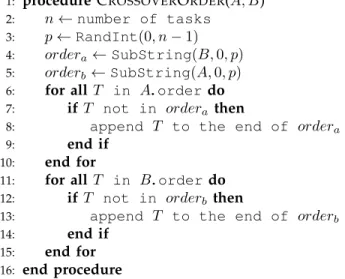
A valid scheduling order must follow the dependencies which exists between tasks. For example, if a task T∗ is a successor of T, T∗ must occur after T in string order. The crossover operation should not violate these restrictions. We design the crossover operator for the order strings as given in Fig. 3. First, the operator randomly chooses a cut-off position, which splits each parent string into two substrings (Step 3). After that, the two first substrings are swapped to be the offspring, and the second substrings are discarded (Steps 4–5). Then, each parentorderstring is scanned from the beginning, with any task that has not occurred in the first substring being appended to the end of this offspring (Steps 6– 10, 11–15). This operator will not cause any dependency conflict since the order of any two tasks should have already existed in at least one parent. An example of this operation is given in Fig. 4, in which the position 3 is randomly chosen as the cut-off position. The first three items in both strings are swapped. Then, the missing tasks for each offspring are appended to its end, in their original orders.
On the other hand, we crossover the stringsins2type and task2instogether. Analogously, the operator first randomly selects a cut-off point, and then, the first parts of two parent task2ins strings are swapped. Here, it is noteworthy that the type of the instance on which a task is running could also be important information for this task, and it is better to keep this relationship. So we make the type of a task follow that task. That is, when task T, running on an instance I of type Pi,
is rescheduled to instance I∗ with type Pj, the type of
I∗ should be changed toPi at the same time. However,
such an operation could potentially break the correspon-dence between other tasks and the types of their hosting instances. For example, a taskTj, which is also scheduled
1: procedure CROSSOVERORDER(A, B)
2: n←number of tasks
3: p←RandInt(0, n−1) 4: ordera←SubString(B,0, p)
5: orderb←SubString(A,0, p)
6: for allT in A.orderdo
7: ifT not in ordera then
8: append T to the end of ordera
9: end if
10: end for
11: for allT in B.orderdo
12: ifT not in orderb then
13: append T to the end of orderb
14: end if
15: end for
16: end procedure
Fig. 3: Crossover operator for stringorder. This opera-tor in place modifies theorderstrings of individualsA andB to produce two offspring.
Fig. 4: An example ofordercrossover.
toI∗and not reassigned, might still prefer an instance of Pj. In this case, the type ofI∗ will be randomly chosen
betweenPiandPj. Otherwise, if there is no such conflict,
a small chance of mutation will be introduced to increase the search ability of the algorithm.
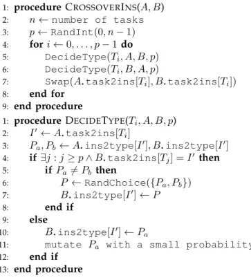
The pseudocode of this operation is given in Fig. 5. Step 3 selects the cut-off point. Before swapping tasks in the first parts (Step 7), an ancillary procedure is invoked. This ancillary procedure, called DecideType, decides on the type of the new hosting instance of task T in individual B, when moving from the instance specified in individualA. For this decision, the types of the new instance (I0), in both individuals, are taken out (P
a and
Pb in Steps 2–3). Then Step 3 decides whether the type
of I0 in B should be changed to Pa or not. If there
is no any task whose index is greater than or equal to the cut-off position p is scheduled to I0 (Step 4), the type of I0 will be changed to Pa (Step 10), with a
mutation performed (Steps 11). Otherwise, the type will be randomly chosen betweenPa and Pb (Steps 5–8).
An example to demonstrate this operator is given in Fig. 6. For illustration, the strings task2ins and ins2typeare presented as the tasks with their hosting instances and the corresponding instance types. After the
1: procedureCROSSOVERINS(A, B) 2: n←number of tasks 3: p←RandInt(0, n−1) 4: fori←0, . . . , p−1 do 5: DecideType(Ti, A, B, p) 6: DecideType(Ti, B, A, p)
7: Swap(A.task2ins[Ti], B.task2ins[Ti])
8: end for
9: end procedure
1: procedureDECIDETYPE(Ti, A, B, p)
2: I0←A.task2ins[Ti] 3: Pa, Pb←A.ins2type[I0], B.ins2type[I0] 4: if∃j:j≥p∧B.task2ins[Tj] =I0 then 5: ifPa 6=Pb then 6: P ←RandChoice({Pa, Pb}) 7: B.ins2type[I0]←P 8: end if 9: else 10: B.ins2type[I0]←P a
11: mutate Pa with a small probability
12: end if
13: end procedure
Fig. 5: Crossover operator for strings Task2Ins and Ins2type and ancillary procedure DecideType. The CrossoverInsprocedure in place modifiestask2ins strings of individualA andB to produce offspring.
cut-off position 3 being randomly chosen, the instance choices and the correspondence instance types of the first three tasks are swapped. For the first individual, the type of I1 which hosts both T2 and T6, is randomly chosen from 2 and 4. Similarly, the final type of instanceI1in the second individual is 4. For this type, the random choice is performed twice, in the DecideTypeinvocations on tasks T0 and T2, since both T0 and T2 are hosted by I1. Additionally, in the first offspring, a mutation is preformed on the type of instanceI3 since this instance is never used after hosting T1. The finaltask2insand
ins2typestrings are given in the bottom of the figure.
4.3.2 Mutation
Like the crossover operators, the mutation operator of string order should not break the task dependencies either. First, we define all successors of taskTi as
succ(Ti) ={Tj |(Ti, Tj)∈D}. (15)
Fig. 7 gives the pseudocode ofordermutation. Starting from task T, the operator searches for a substring in which each task is neither a predecessor nor a successor of T (Steps 4–10). Then, T is moved to a randomly chosen new position inside this substring (Steps 11– 12). On each direction, the search procedure starts from the position of T, and stops once the current task is either in pred(T) or in succ(T). Fig. 8 demonstrates an example where task 2 is randomly chosen to be the mutation point. A search is then performed to find the
Fig. 6: An example of task2ins and ins2type crossover.
1: procedure MUTATEORDER(X, pos)
2: n←number of tasks
3: T ←X.order[pos] 4: start, end←pos
5: whilestart≥0∧X.order[start]∈/pred(T)do
6: start←start−1
7: end while
8: whileend < n∧X.order[end]∈/succ(T)do
9: end←end+ 1
10: end while
11: pos0←RandInt(start+ 1, end−1) 12: Move T to pos0 in X.order
13: end procedure
Fig. 7: Mutation operator for order strings. Given a position pos, this operator randomly moves the posth task inX.order to another valid position.
Fig. 8: An example of ordermutation.
substring meeting the conditions, between task 1 and task 4. Finally, task 2 is randomly moved to a new position inside this substring.
ins2type is performed by a classical operator, that is, randomly generating a new valid value for each position, with a small probability.
4.4 Initial Population
In the workflow scheduling problem, the search space of solutions is typically huge, especially when a large workflow is involved, which could cause evolutionary algorithms very slow to converge. In our algorithm, to accelerate the search procedure, the initial population consists of the individuals generated by different initial-ization methods. Assuming the size of population is n, these individuals include
• a schedule computed by HEFT, which is treated as
the fastest schedule,
• a “cheapest” schedule produced at the same time
when executing HEFT, as an estimate of the cheap-est schedule,
• n−2 random schedules initialized by a procedure namedRandTypeOrIns.
First, HEFT is slightly extended for guessing an indi-vidual that can approach the cheapest cost, along with the standard procedure of finding the fastest schedule. This cheapest schedule is produced by assigning the task to the instance which can minimize the currently-generated cost in the processor selection phase of each task. This individual might not be the actual cheapest one; in spite of that, it could still be seen as a rough approximation of one endpoint of the Pareto front. At the same time, the fastest individual produced by the original HEFT could be used as another approximate endpoint.
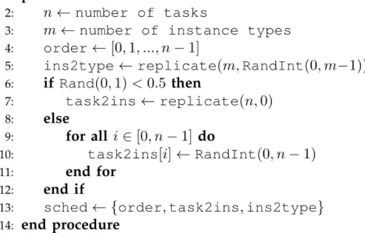
Besides these two heuristic-generated schedules, we initialize other individuals randomly. For each individ-ual, the procedure is presented in Fig. 9. First, the string order is simply constructed as an increasing sequence [0,1, ...n−1] (line 4). Then, a specific instance type is randomly chosen, and all instances will share this type, by setting all bits of the ins2type string to the index of this type (line 5). Finally, the string task2ins is initialized by a random choice of two methods, with equal probability (line 6). The first method is to put all tasks in a single instance, by setting all bits oftask2ins to0 (line 7). Another method is to put tasks in different instances at random, by randomly choosing an integer from [0, n−1]for each bit of task2ins(lines 9-10).
4.5 Complexity Analysis
The time complexity for both CrossoverOrder and MutateOrderisO(n), wherenis the number of tasks. The time complexity of the procedureCrossoverInsis O(n2), because for each swapped instance in the string
task2ins, an O(n) scan is needed to find whether it also hosts another task according to the opposite individ-ual. The evaluation procedure for each individual has an O(e)time complexity. For a given DAG, the number of
1: procedure RANDTYPEORINS
2: n←number of tasks
3: m←number of instance types
4: order←[0,1, ..., n−1]
5: ins2type←replicate(m,RandInt(0, m−1)) 6: ifRand(0,1)<0.5 then
7: task2ins←replicate(n,0) 8: else
9: for alli∈[0, n−1]do
10: task2ins[i]←RandInt(0, n−1)
11: end for
12: end if
13: sched← {order,task2ins,ins2type}
14: end procedure
Fig. 9: The RandTypeOrInsprocedure.
edges could be at mostn2, so the time complexity of each evaluation is on the order of O(n2). Thus, the overall complexity of the evolution is on the order of O(kgn2), with kindividuals in population andg generations.
Besides the evolution procedure, when initializing the first population, HEFT is performed once. The HEFT algorithm hasO(sn2)complexity wheresis the number of available services [23]. By using the Cloud-aware ex-tension proposed in [22], a heterogeneous environment can be constructed bym×ninstances in Cloud, where mis the number of instance types. Thus, HEFT has the time complexity ofO(mn3)in our initialization scheme. Above all, the overall computational complexity of our proposed algorithm is on the order ofO(mn3+kgmn2). However, we would like to point out that, when exe-cuting HEFT in the population initialization procedure, because a) most instances in the simulated service pool are not used at all, and b) several unused instances are actually identical if they also share a same type, a large number of redundant calculations could be eliminated or optimized if using proper data structures. Also, in practice,m×nis usually much less thenk×g. For these reasons, we observed that the most time-consuming parts in SPEA2* and our proposed EMS-C are still the evolution procedures, with the complexity ofO(kgn2).
5
E
XPERIMENTS5.1 Experiments Parameters
5.1.1 IaaS Model
The experiments are based on the instance specifications and pricing scheme of Amazon EC2. The General Purpose instance group in US East region with the purchasing option of On-Demand Instance is used. Table 1 gives the used parameters.
5.1.2 Workflows
Pegasus project has published the workflow of a num-ber of real-world applications including Montage, Cy-berShake, Epigenomics, LIGO Inspiral Analysis and
TABLE 1: IaaS parameters used in experiments.
Instance Type Compute Unit Bandwidth (bytes/sec) Price ($) m1.small 1.7 39,321,600 0.06 m1.medium 3.75 85,196,800 0.12 m3.medium 3.75 85,196,800 0.113 m1.large 7.5 85,196,800 0.24 m3.large 7.5 85,196,800 0.225 m1.xlarge 15 131,072,000 0.48 m3.xlarge 15 131,072,000 0.45 m3.2xlarge 30 131,072,000 0.9
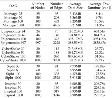
TABLE 2: Characteristics of the real-world DAGs.
DAG of NodesNumber of EdgesNumber Data SizeAverage Runtime (cu=1)Average Task
Montage 25 25 95 3.43MB 8.44s Montage 50 50 206 3.36MB 9.78s Montage 100 100 433 3.23MB 10.58s Montage 1000 1000 4485 3.21MB 11.36s Epigenomics 24 24 75 116.20MB 681.54s Epigenomics 46 46 148 104.81MB 844.93s Epigenomics 100 100 322 395.10MB 3954.90s Epigenomics 997 997 3228 388.59MB 3858.67s CyberShake 30 30 112 747.48MB 23.77s CyberShake 50 50 188 864.74MB 29.32s CyberShake 100 100 380 849.60MB 31.53s CyberShake 1000 1000 3988 102.29MB 22.71s Sipht 30 30 91 7.73MB 178.92s Sipht 60 60 198 6.95MB 194.48s Sipht 100 100 335 6.27MB 175.55s Sipht 1000 1000 3528 5.91MB 179.05s Inspiral 30 30 95 9.00MB 206.78s Inspiral 50 50 160 9.16MB 226.19s Inspiral 100 100 319 8.93MB 206.12s Inspiral 1000 1000 3246 8.90MB 227.25s
* When calculating the number of edges, average data size and average task runtime, the pseudo entry/exit node and the related edges are included.
SIPHT [36], [37]. For each workflow, the published de-tails include the DAG, the sizes of data transferring and the reference execution time based on [email protected] CPUs (cu≈8). These workflows have been widely used for measuring the performance of scheduling algorithms, and we thus include these workflows in our exper-iments. The DAG characteristics of these workflows, including the numbers of nodes and edges, average data size and average task runtime, are given in Table. 2, and the sample structures of different applications are given in Fig. 10.
Besides these real-world workflows, we also test our algorithm on random workflows. The random work-flows are generated by a tool which was also used by [19], using the parameters width, regularity, density, jumps and the number of tasks n. We first generate 100 DAGs using random n ∈ [10,100], jump ∈ {1,2,3}, regularity ∈ {0.2,0.4,0.6}, width ∈ {0.2,0.4,0.6} and density ∈ {0.2,0.4,0.8}. In this tool, the execution time of tasks are given as CPU cycles. We notice that, for most generated tasks, the execution time is less than one hour when running on a 2GHz CPU. However, the pricing scheme we used has a minimum charging time of one hour. To improve the coverage of
(a) Montage (b) Epigenomics (c) Inspiral
(d) CyberShake (e) Sipht
Fig. 10: Structures of the real-world workflows.
our experiments, we enlarge the execution time of every task by 60 times to produce another 100 workflows, and repeat the experiments on both workflow sets. These two random workflow sets are respectively called as ‘random (quick)’ and ‘random (slow)’ in following discussions.
5.1.3 EMO Frameworks
We have applied our proposed genetic operations and encoding scheme above to several popular EMO fromeworks including NSGA-II [32], MOEA/D [38] and SPEA2 [39]. Under different frameworks, the non-dominated fronts obtained by our designs are similar. Due to the space limit, we only present the experimental results under NSGA-II here.
As a classic Pareto-based EMO framework, NSGA-II introduces two effective selection criteria, Pareto non-dominated sorting and crowding distance, to guide the search towards the optimal front. The Pareto non-dominated sorting is used to divide the individuals into several ranked non-dominated fronts according to their dominance relations. The crowding distance is used to estimate the density of the individuals in a population. NSGA-II prefers two kinds of individuals: 1) the indi-viduals with lower rank or 2) the indiindi-viduals with larger crowding distance if their rank is the same.
For convenience, our proposed approach, under the NSGA-II framework, is denoted as ‘Evolutionary Multi-objective Scheduling for Cloud (EMS-C)’ algorithm in discussions below. Like most existing EMO algorithms, EMS-C will terminate if the function evaluations reach a preset number. The outcome of the algorithm is the final population with the results in both decision and objective spaces.
5.1.4 Compared Algorithms
We compare EMS-C with several QoS optimization scheduling algorithms, including MOHEFT, NSPSO, ε -Fuzzy PSO, SPEA2* and MODE. Except for MOHEFT, all these algorithms assume the Grid-like environments rather than Cloud platforms. Along with MOHEFT,
a cloud-aware extension has been proposed to make existing list-based algorithms can be used with the IaaS model [22]. In this extension, the IaaS platform is simulated as a common heterogeneous environment by constructing an instance pool from Cloud in advance. For a DAG with n tasks and an IaaS platform with m instance types, n×m instances are prepared, with n instances for each type. We apply this extension to all the algorithms except our EMS-C in the experiments.
In addition, the following setups are used:
• For MOHEFT, the number of trade-off solutions is
50 (k= 50).
• For all NSPSO, ε-Fuzzy PSO, MODE, SPEA2* and
our algorithm, the size of population is 50 and the number of generations is 1000.
• For both SPEA2* and EMS-C, the probabilities of
crossover and mutation are 1and 1/n, respectively.
• Forε-Fuzzy PSO, the corresponding parameters are
c1 = 2.5 → 0.5, c2 = 0.5 → 2.5, ε = 0.1 and the inertia weight w= 0.9→0.1, as used in [21].
• For NSPSO, the corresponding parameters are w= 1.0→0.4,c1= 2 andc2= 2, as used in [40].
• On each workflow, the scheduling is repeated for 10
times for all algorithms except MOHEFT.
5.1.5 Performance Metric
Hypervolume (HV) [41] is one of the most popular performance metrics in the EMO area. Calculating the volume of the objective space between the obtained solution set and the reference point, HV can provide a combined information about convergence and diversity of the set. A larger HV value is preferable, which indi-cates that the solution set is close to the Pareto front and also has a good distribution.
To compare the schedules of totally different work-flows, we normalize the produced solutions on each workflow as follows. First, the solutions produced by all the tested algorithms under all the executions are mixed and non-dominated solutions are selected from this mixed set. These non-dominated solutions are used as an approximation of the actual Pareto front and all results dominated by this approximating Pareto front are discarded. Then, the makespans and the costs are separately normalized by dividing their upper bounds of the approximation. After all the results are normalized, a reference point (1.1,1.1) is used in the calculations of HV, according to the recommendation in [34].
The HV results of a solution set could be zero if there is no solution in or close enough to the Pareto front approximation [42]. Numeric comparing other HV with such a zero value is meaningless [43]. Thus, we consider this case as afailurefor the corresponding algorithm, since its performance is significantly worse than those in this case. The number of the failures is also considered as one metric in the comparative experiments.
TABLE 3: Time complexity of EMS-C and the compared algorithms when applied in Cloud.
Algorithm EMS-C SPEA2* MODE
T(n) O((mn3+kgn2) O(mn3+kgn2) O(kgn2) Algorithm NSPSO ε-Fuzzy PSO MOHEFT
T(n) O(kgmn2) O(kgmn2) O(k2m2n3)
5.2 Results and Discussions
5.2.1 Cloud Scheduling Algorithm Complexity
Before presenting the experimental results, we first an-alyze the time complexity of the compared algorithms. The complexity of some compared algorithms has been given in their original literatures [6], [9], [11], [21], [22]. However, due to the different resource management models, the time and/or space complexity of these al-gorithms might be changed when being applied in IaaS. We assume that n is the number of tasks in a given DAG,mis the number of instance types,gis the number of iterations for GA and PSO, and k is the population size for GA and PSO as well as the size of the trade-off set in MOHEFT. Additionally, the simulated Grid-like available service set, as discussed in Section 5.1.4, is constructed in advance with the sizes=m×n.
Since SPEA2* is also EMO-based and uses O(sn2) GD/TD heuristic in the population initialization as well, its time complexity should be also O(mn3 +kgn2). In practice, because that the genetic operators used by SPEA2* (O(n)) are simpler than those in EMS-C (O(n2)), the actual execution time of SPEA2* might be slightly less than ours in some cases. Similarly, the most time-consuming part of MODE is also the individual evalua-tions which have the complexity ofO(n2). Therefore, the overall time complexity for MODE isO(kgn2).
Forε-Fuzzy PSO and NSPSO, the complexity of eval-uating all particle positions is also O(kgn2). However, in these algorithms, s × n size matrices are used to represent both the particle positions and the velocities. According to the literatures [11], [21], these matrices need to be updated in every iteration, and all these oper-ations are(O(sn) =O(mn2)). For this reason, the actual overall time complexity of ε-Fuzzy PSO and NSPSO is O(kgmn2)in Cloud. Additionally, we observe in practice that, due to the large amount of memory acquired for storing these matrices, and the frequent operations on the memory, the executions of these PSO algorithms might be slower, especially when the algorithms are implemented in a high-level programming language.
MOHEFT is extended on the basis of HEFT, which maintains k trade-offs during its processor selection phase. Since HEFT is(O(sn2) =O(mn3))[23], MOHEFT would be at least O(kmn3). On the other hand, the procedure of the non-dominated sorting and crowding distance sorting is with the complexity of O(q2) [32], where q is the number of all newly extended interme-diate schedules. However, by using the Cloud aware
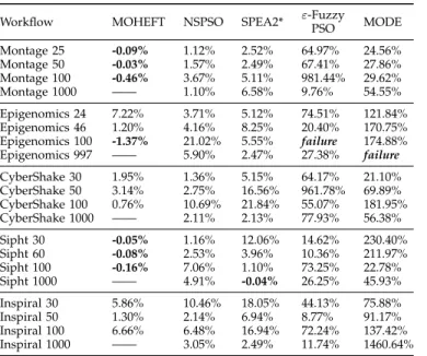
TABLE 4: HV differences between EMS-C and the peer algorithms on the real-world workflows (i.e., HV(EMS-C)/HV(peer algorithm)×100%−1).
Workflow MOHEFT NSPSO SPEA2* ε-FuzzyPSO MODE
Montage 25 -0.09% 1.12% 2.52% 64.97% 24.56% Montage 50 -0.03% 1.57% 2.49% 67.41% 27.86% Montage 100 -0.46% 3.67% 5.11% 981.44% 29.62% Montage 1000 —— 1.10% 6.58% 9.76% 54.55% Epigenomics 24 7.22% 3.71% 5.12% 74.51% 121.84% Epigenomics 46 1.20% 4.16% 8.25% 20.40% 170.75% Epigenomics 100 -1.37% 21.02% 5.55% failure 174.88% Epigenomics 997 —— 5.90% 2.47% 27.38% failure CyberShake 30 1.95% 1.36% 5.15% 64.17% 21.10% CyberShake 50 3.14% 2.75% 16.56% 961.78% 69.89% CyberShake 100 0.76% 10.69% 21.84% 55.07% 181.95% CyberShake 1000 —— 2.11% 2.13% 77.93% 56.38% Sipht 30 -0.05% 1.16% 12.06% 14.62% 230.40% Sipht 60 -0.08% 2.53% 3.96% 10.36% 211.97% Sipht 100 -0.16% 7.06% 1.10% 73.25% 22.78% Sipht 1000 —— 4.91% -0.04% 26.25% 45.93% Inspiral 30 5.86% 10.46% 18.05% 44.13% 75.88% Inspiral 50 1.30% 2.14% 6.94% 8.77% 91.17% Inspiral 100 6.66% 6.48% 16.94% 72.24% 137.42% Inspiral 1000 —— 3.05% 2.49% 11.74% 1460.64%
extension in [22],qwould be equal tok×m×n. Therefore, the SortCrowdDist procedure in MOHEFT has time complexity of O(k2m2n2), leading to the overall algo-rithm with the time complexity as high asO(k2m2n3).
The time complexity of all the peer algorithms and EMS-C are listed in Table 3.
5.2.2 The Real-World Workflows
The HV improvements for EMS-C against the peer algo-rithms are presented in Table. 4. As can be seen from the table, EMS-C performs significantly better than NSPSO, SPEA2*, ε-Fuzzy PSO and MODE for all the real-world cases, except for Sipht 1000 on which SPEA2* can achieve slightly better HV. Also, EMS-C performs better than MOHEFT on all the CyberShake and Inspiral workflows, as well as the small-size Epigenomics workflows, with the improvements range from 0.76% to 7.22 %. In Epige-nomics 100 cases, MOHEFT achieves noticeable better HV than EMS-C, for which the difference is 1.37%. Be-sides that, MOHEFT also slightly outperforms EMS-C on the small/medium-size Sipht and Montage workflows; however, the differences are much smaller, most of which are less than 0.1%. Due to the high time complexity in Cloud, MOHEFT is not able to finish in acceptable time on all the large-size workflows.
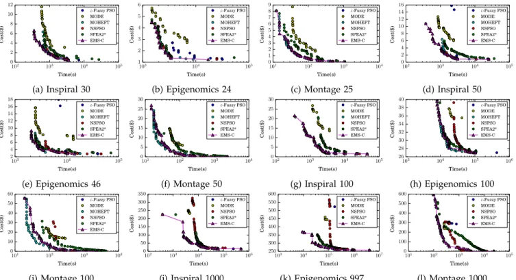
We plot the produced makespan-cost trade-offs for different algorithms on the Inspiral, Epigenomics and Montage workflows in Fig. 11. Noted that the x-axes are all logarithmic. These plots indicate that, even in the cases where MOHEFT performs the best, the trade-off fronts obtained by EMS-C are still significantly superior to those obtained by the rest of the peer algorithms.
The runtime comparisons for different algorithms to schedule the real-world workflows are presented in Table 5. Here we compute and compare the runtime
TABLE 5: Runtime ratios of the peer algorithms against the proposed EMS-C on the real-world workflows (i.e., runtime(peer algorithm)/runtime(EMS-C)).
Workflow SPEA2* MODE NSPSO ε-FuzzyPSO MOHEFT
Montage 25 1.91 1.35 22.32 13.37 3.76 Montage 50 1.43 1.40 30.15 25.99 35.97 Montage 100 1.13 1.35 46.42 45.43 131.84 Montage 1000 0.29 1.01 66.06 61.52 —— Epigenomics 24 1.79 1.19 24.97 13.43 0.19 Epigenomics 46 1.26 1.36 30.09 25.27 1.01 Epigenomics 100 0.91 1.16 47.53 44.46 34.52 Epigenomics 997 0.23 1.05 83.59 82.96 —— CyberShake 30 1.62 1.18 21.25 15.04 10.39 CyberShake 50 1.28 1.37 30.17 26.81 38.16 CyberShake 100 0.92 1.31 44.75 42.22 110.42 CyberShake 1000 0.32 0.97 70.72 69.56 —— Sipht 30 1.54 1.08 22.46 15.03 0.27 Sipht 60 1.07 1.19 29.64 27.41 1.69 Sipht 100 0.83 1.16 41.00 41.10 14.23 Sipht 1000 0.28 1.06 74.25 71.02 —— Inspiral 30 1.68 1.28 23.88 16.03 0.79 Inspiral 50 1.27 1.12 29.04 26.01 2.49 Inspiral 100 0.90 1.52 45.73 47.06 25.18 Inspiral 1000 0.24 1.04 71.91 73.01 ——
ratios between the peer algorithms and EMS-C, that is, if the ratio is larger than 1, EMS-C is shown to be faster than the competitor. Due to its simplest genetic operators, SPEA2* runs faster than EMS-C in many cases. Nevertheless, the overall time complexity of SPEA2* and EMS-C is the same (O(kgn2)). On the other hand, MODE has the similar execution time to EMS-C, which is because the time complexity of calculating the Ulam distances is O(n2) as well. Compared with the genetic algorithms, PSO algorithms perform much slowly, due to their higher time complexity and frequent memory operations, especially when the number of tasks is large. Finally, it is worth pointing out that the execution time of MOHEFT increases rapidly with the number of tasks, and it fails to finish in acceptable time on all the large-size real-world workflows.
5.2.3 The Random Workflows
Since the random workflow sets consist of totally dif-ferent workflows, the results are hard to be compared directly. Thus, we also compare the HV ratios between the compared algorithm and EMS-C on each tested workflow. That is, if the ratio is less than 1, EMS-C is shown to perform better than the competitor.
Fig. 12a gives the box plots for the HV ratios on the quick random workflows. The figure shows that EMS-C clearly outperforms ε-Fuzzy PSO, MODE, NSPSO and SPEA2* in all these quick random cases. MOHEFT performs remarkably better than all the other compared algorithms. However, EMS-C can still defeat MOHEFT in most cases, although the differences are small.
In contrast, the slow random workflows are much harder to schedule for all the tested algorithms. The HV ratio statistic for the slow workflows is presented in Fig. 12b. The plot indicates that EMS-C can still
102 103 104 105 Time(s) 0 2 4 6 8 10 12 C os t( $) ε-Fuzzy PSO MODE MOHEFT NSPSO SPEA2* EMS-C (a) Inspiral 30 103 104 105 Time(s) 1 2 3 4 5 6 C os t( $) ε-Fuzzy PSO MODE MOHEFT NSPSO SPEA2* EMS-C (b) Epigenomics 24 101 102 103 104 Time(s) 0 1 2 3 4 5 6 7 8 9 C os t( $) ε-Fuzzy PSO MODE MOHEFT NSPSO SPEA2* EMS-C (c) Montage 25 102 103 104 105 Time(s) 0 2 4 6 8 10 12 14 16 C os t( $) ε-Fuzzy PSO MODE MOHEFT NSPSO SPEA2* EMS-C (d) Inspiral 50 103 104 105 Time(s) 2 4 6 8 10 12 14 16 18 C os t( $) ε-Fuzzy PSO MODE MOHEFT NSPSO SPEA2* EMS-C (e) Epigenomics 46 101 102 103 104 Time(s) 0 5 10 15 20 25 30 C os t( $) ε-Fuzzy PSO MODE MOHEFT NSPSO SPEA2* EMS-C (f) Montage 50 102 103 104 105 Time(s) 0 5 10 15 20 25 30 C os t( $) ε-Fuzzy PSO MODE MOHEFT NSPSO SPEA2* EMS-C (g) Inspiral 100 103 104 105 106 Time(s) 26 28 30 32 34 36 38 40 C os t( $) ε-Fuzzy PSO MODE MOHEFT NSPSO SPEA2* EMS-C (h) Epigenomics 100 101 102 103 104 Time(s) 0 10 20 30 40 50 60 C os t( $) ε-Fuzzy PSO MODE MOHEFT NSPSO SPEA2* EMS-C (i) Montage 100 102 103 104 105 106 Time(s) 0 50 100 150 200 250 300 350 C os t( $) ε-Fuzzy PSO MODE NSPSO SPEA2* EMS-C (j) Inspiral 1000 103 104 105 106 107 Time(s) 250 300 350 400 450 500 550 600 C os t( $) ε-Fuzzy PSO MODE NSPSO SPEA2* EMS-C (k) Epigenomics 997 101 102 103 104 105 Time(s) 0 100 200 300 400 500 600 C os t( $) ε-Fuzzy PSO MODE NSPSO SPEA2* EMS-C (l) Montage 1000 Fig. 11: Makespan-time trade-offs for some real-world workflows.
significantly outperform ε-Fuzzy PSO and MODE in all cases, and can obtain better trade-offs than NSPSO amd SPEA2* in most cases. In addition, compared with MOHEFT, EMS-C has shown a clearer advantage than on the quick workflows.
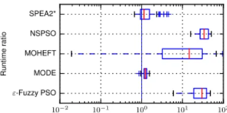
The runtime ratios on the random workflows are plotted in Fig. 13. The plot indicates that, although in some cases the qualities of their obtained results are similar to or even better than EMS-C, MOHEFT, NSPSO and ε-Fuzzy PSO usually incur much more time. This observation conforms the analysis in Section 5.2.1.
We present the trade-off plots for some selected ran-dom workflows in Fig. 14. No. 96 in the quick set and No. 47 in the slow set are the cases where EMS-C performs remarkably better than all the competitors; NO. 44 in the quick set and No. 24 in the slow set are the cases where both MOHEFT and EMS-C perform equally well; No. 2 in the quick set and No. 13 in the slow set are the cases where MOHEFT performs the best. The figures show that, EMS-C can obtain trade-off fronts with clear advantage over the competitors in the cases where it performs the best. At the same time, in the cases where MOHEFT performs slightly better, EMS-C can still generate acceptable solutions that are pretty close to the optimal ones. In addition, it is worth noting that, in Fig. 14f, although MOHEFT can find some solutions Pareto-dominating our obtained schedules, EMS-C can also produce faster schedules that MOHEFT cannot find. Table 6 gives the failure numbers experienced by each algorithm on the random workflows. Only MODE has failures on the quicker set (17). On the slower workflows,
0.0 0.2 0.4 0.6 0.8 1.0 1.2 ε-Fuzzy PSO MODE MOHEFT NSPSO SPEA2* H yp er vo lu m e ra tio
(a) On the random (quick) workflows
0.0 0.5 1.0 1.5 2.0 ε-Fuzzy PSO MODE MOHEFT NSPSO SPEA2* H yp er vo lu m e ra tio
(b) On the random (slow) workflows
Fig. 12: Box plots for the HV ratios of the peer algorithm against the proposed EMS-C on the random workflows (i.e.,HV(peer algorithm)/HV(EMS-C)).
TABLE 6: Number of failures experienced by the peer algorithms and EMS-C on the random workflows.
EMS-C
(both) SPEA2* MOHEFT NSPSO
ε-Fuzzy
PSO MODE
Quick 0 0 0 0 0 17
Slow 0 0 1 2 16 12
MOHEFT fails once and NSPSO fails twice. In addition to that, bothε-Fuzzy PSO and MODE fail in more than 10 cases (16 and 12, respectively). In contrast, EMS-C
expe-10−2 10−1 100 101 102 ε-Fuzzy PSO MODE MOHEFT NSPSO SPEA2* R un tim e ra tio
Fig. 13: Box plots for the runtime ratios of the peer algo-rithm against the proposed EMS-C on the random work-flows (i.e., runtime(peer algorithm)/runtime(EMS-C)).
102 103 104 105 Time(s) 0 2 4 6 8 10 12 14 16 18 C os t( $) ε-Fuzzy PSO MODE MOHEFT NSPSO SPEA2* EMS-C
(a) No. 96 (quick)
104 105 106 Time(s) 8 9 10 11 12 13 14 C os t( $) ε-Fuzzy PSO MODE MOHEFT NSPSO SPEA2* EMS-C (b) No. 47 (slow) 102 103 104 105 Time(s) 0 2 4 6 8 10 12 C os t( $) ε-Fuzzy PSO MODE MOHEFT NSPSO SPEA2* EMS-C (c) No. 44 (quick) 104 105 106 Time(s) 20 25 30 35 40 45 50 55 60 C os t( $) ε-Fuzzy PSO MODE MOHEFT NSPSO SPEA2* EMS-C (d) No. 24 (slow) 103 104 105 Time(s) 0 1 2 3 4 5 6 7 8 9 C os t( $) ε-Fuzzy PSO MOHEFT NSPSO SPEA2* EMS-C
(e) No. 2 (quick)
104 105 106 Time(s) 40 50 60 70 80 90 100 C os t( $) ε-Fuzzy PSO MODE MOHEFT NSPSO SPEA2* EMS-C (f) No. 13 (slow) Fig. 14: Trade-offs for selected random workflows.
riences no failure on any set under any framework. The results have strengthened the previous findings that for the Cloud workflow scheduling problem, our proposed evolutionary algorithm is more stable and appears to be much more likely to produce acceptable schedules.
6
C
ONCLUSIONAlthough there are many existing workflow scheduling algorithms for the multi-processor architectures or het-erogeneous computing environments, they have difficul-ties in being directly applied to the Cloud environments. In this paper, we try to address this by modeling the workflow scheduling problem in Cloud as a multi-objective optimization problem where we have consid-ered the real-world Cloud computing models.
To solve the multi-objective Cloud scheduling prob-lem which minimizes both makespan and cost simul-taneously, we propose a novel encoding scheme which represents all the scheduling orders, task-instance as-signments and instance specification choices. Based on
this scheme, we also introduce a set of new genetic operators, the evaluation function and the population initialization scheme for this problem. We apply our de-signs to several popular EMO frameworks, and test the proposed algorithm on both the real-world workflows and two sets of randomly generated workflows. The ex-tensive experiments are based on the actual pricing and resource parameters of Amazon EC2, and results have demonstrated that this algorithm is highly promising with potentially wide applicability.
As parts of our future work, we will consider using more than one pricing schemes, instance type groups or even multi-Clouds in a single schedule. Furthermore, the monetary costs and time overheads of both communica-tion and storage will be included in the consideracommunica-tions.
R
EFERENCES[1] P. Mell and T. Grance, “The nist definition of cloud computing,” National Institute of Standards and Technology, Tech. Rep. 6, 2009. [2] B. Martens, M. Walterbusch, and F. Teuteberg, “Costing of cloud computing services: A total cost of ownership approach,” in45th Hawaii Int. Conf. Syst. Sci. IEEE, 2012, pp. 1563–1572.
[3] E. Deelman, G. Singh, M.-H. Su, J. Blythe, Y. Gil, C. Kesselman, G. Mehta, K. Vahi, G. B. Berriman, J. Good et al., “Pegasus: A framework for mapping complex scientific workflows onto distributed systems,” Sci. Programming, vol. 13, no. 3, pp. 219– 237, 2005.
[4] T. Fahringer, R. Prodan, R. Duan, F. Nerieri, S. Podlipnig, J. Qin, M. Siddiqui, H.-L. Truong, A. Villazon, and M. Wieczorek, “Askalon: A grid application development and computing envi-ronment,” in6th IEEE/ACM Int. Workshop on Grid Comput. IEEE Computer Society, 2005, pp. 122–131.
[5] G. Juve, M. Rynge, E. Deelman, J.-S. Vockler, and G. B. Berriman, “Comparing futuregrid, amazon ec2, and open science grid for scientific workflows,”Computing in Sci. & Eng., vol. 15, no. 4, pp. 20–29, 2013.
[6] J. Yu, M. Kirley, and R. Buyya, “Multi-objective planning for workflow execution on grids,” in8th IEEE/ACM Int. Conf. on Grid Comput. IEEE Computer Society, 2007, pp. 10–17.
[7] M. Wieczorek, A. Hoheisel, and R. Prodan, “Towards a general model of the multi-criteria workflow scheduling on the grid,” Future Generation Comput. Syst., vol. 25, no. 3, pp. 237–256, 2009. [8] W.-N. Chen and J. Zhang, “An ant colony optimization approach to a grid workflow scheduling problem with various QoS require-ments,”IEEE Trans. Syst. Man Cybern. A., Syst. Humans, vol. 39, no. 1, pp. 29–43, 2009.
[9] A. Talukder, M. Kirley, and R. Buyya, “Multiobjective differential evolution for scheduling workflow applications on global grids,” Concurrency and Computation: Practice and Experience, vol. 21, no. 13, pp. 1742–1756, 2009.
[10] F. Zhang, J. Cao, K. Hwang, and C. Wu, “Ordinal optimized scheduling of scientific workflows in elastic compute clouds,” in 3rd IEEE Int. Conf. Cloud Comput. Technol. and Sci. IEEE, 2011, pp. 9–17.
[11] R. Garg and A. K. Singh, “Multi-objective workflow grid schedul-ing based on discrete particle swarm optimization,” in Swarm, Evolutionary, and Memetic Comput. Springer, 2011, pp. 183–190. [12] M. Zhu, Q. Wu, and Y. Zhao, “A cost-effective scheduling
al-gorithm for scientific workflows in clouds,” in 31th IEEE Int. Performance Comput. and Commun. Conf. IEEE, 2012, pp. 256–265. [13] O. Udomkasemsub, L. Xiaorong, and T. Achalakul, “A multiple-objective workflow scheduling framework for cloud data analyt-ics,” in24th IEEE Int. Joint Conf. Comput. Sci. and Softw. Eng. IEEE, 2012, pp. 391–398.
[14] M. Malawski, G. Juve, E. Deelman, and J. Nabrzyski, “Cost-and deadline-constrained provisioning for scientific workflow ensembles in iaas clouds,” inInt. Conf. High Performance Comput., Networking, Storage and Analysis. IEEE Computer Society Press, 2012, p. 22.
[15] S. Su, J. Li, Q. Huang, X. Huang, K. Shuang, and J. Wang, “Cost-efficient task scheduling for executing large programs in the cloud,”Parallel Comput., vol. 39, no. 4, pp. 177–188, 2013. [16] W. Zheng and R. Sakellariou, “Budget-deadline constrained
work-flow planning for admission control,”J. of Grid Comput., vol. 11, no. 4, pp. 633–651, 2013.
[17] N. D. Man and E.-N. Huh, “Cost and efficiency-based scheduling on a general framework combining between cloud computing and local thick clients,” inInt. Conf. Comput., Manage. and Telecommun. IEEE, 2013, pp. 258–263.
[18] S. Abrishami, M. Naghibzadeh, and D. H. Epema, “Deadline-constrained workflow scheduling algorithms for infrastructure as a service clouds,”Future Generation Comput. Syst., vol. 29, no. 1, pp. 158–169, 2013.
[19] H. Arabnejad and J. G. Barbosa, “A budget constrained schedul-ing algorithm for workflow applications,”J. of Grid Comput., pp. 1–15, 2014.
[20] H. M. Fard, R. Prodan, and T. Fahringer, “Multi-objective list scheduling of workflow applications in distributed computing infrastructures,”J. of Parallel and Distrib. Comput., vol. 74, no. 3, pp. 2152–2165, 2014.
[21] R. Garg and A. K. Singh, “Multi-objective workflow grid schedul-ing usschedul-ingε-fuzzy dominance sort based discrete particle swarm optimization,”J. of Supercomputing, vol. 68, no. 2, pp. 709–732, 2014.
[22] J. J. Durillo and R. Prodan, “Multi-objective workflow scheduling in amazon ec2,”Cluster Comput., vol. 17, no. 2, pp. 169–189, 2014. [23] H. Topcuoglu, S. Hariri, and M.-y. Wu, “Performance-effective and low-complexity task scheduling for heterogeneous computing,” IEEE Trans. Parallel Distrib. Syst, vol. 13, no. 3, pp. 260–274, 2002. [24] R. Sakellariou, H. Zhao, E. Tsiakkouri, and M. D. Dikaiakos, “Scheduling workflows with budget constraints,” in Integrated Research in GRID Comput. Springer, 2007, pp. 189–202.
[25] I. Foster, Y. Zhao, I. Raicu, and S. Lu, “Cloud computing and grid computing 360-degree compared,” inGrid Comput. Environments Workshop. IEEE, 2008, pp. 1–10.
[26] C. Computing. (2013, Nov.) Back to the future: 1.21 petaflops(rpeak), 156,000-core cyclecloud HPC runs 264 years of materials science. [Online]. Available: http://goo.gl/59ItjU [27] H. Liu. (2014, Feb.) Amazon ec2 grows 62% in 2 years. [Online].
Available: http://goo.gl/FgkxoR
[28] M. Rosoff. (2015, Apr.) Amazon’s true brilliance shone this week in a tale of three clouds. Business Insider. [Online]. Available: http://goo.gl/D6GhW1
[29] I. Amazon Web Services. (2014) Amazon ec2 pricing. [Online]. Available: http://goo.gl/yKb41s
[30] Microsoft. (2014) Virtual machines pricing details. [Online]. Available: http://goo.gl/UrDkvF
[31] Google. (2014) Google compute engine pricing. [Online]. Available: http://goo.gl/fKQwzb
[32] K. Deb, A. Pratap, S. Agarwal, and T. Meyarivan, “A fast and elitist multiobjective genetic algorithm: Nsga-ii,”IEEE Trans. Evol. Comput., vol. 6, no. 2, pp. 182–197, 2002.
[33] H. Li and Q. Zhang, “Multiobjective optimization problems with complicated pareto sets, moea/d and nsga-ii,”IEEE Trans. Evol. Comput., vol. 13, no. 2, pp. 284–302, 2009.
[34] H. Ishibuchi, Y. Hitotsuyanagi, N. Tsukamoto, and Y. Nojima, “Many-objective test problems to visually examine the behavior of multiobjective evolution in a decision space,” inParallel Problem Solving from Nature. Springer, 2010, pp. 91–100.
[35] M. Li, S. Yang, and X. Liu, “Shift-based density estimation for pareto-based algorithms in many-objective optimization,” IEEE Trans. Evol. Comput., vol. 18, no. 3, pp. 348–365, 2014.
[36] S. Bharathi, A. Chervenak, E. Deelman, G. Mehta, M.-H. Su, and K. Vahi, “Characterization of scientific workflows,” in3rd Workshop on Workflows in Support of Large-Scale Sci. IEEE, 2008, pp. 1–10.
[37] G. Juve, A. Chervenak, E. Deelman, S. Bharathi, G. Mehta, and K. Vahi, “Characterizing and profiling scientific workflows,” Fu-ture Generation Comput. Syst., vol. 29, no. 3, pp. 682–692, 2013. [38] Q. Zhang and H. Li, “Moea/d: A multiobjective evolutionary
algorithm based on decomposition,”IEEE Trans. Evol. Comput., vol. 11, no. 6, pp. 712–731, 2007.
[39] E. Zitzler, M. Laumanns, L. Thiele, E. Zitzler, E. Zitzler, L. Thiele, and L. Thiele, “Spea2: Improving the strength pareto evolutionary algorithm,” Eidgenössische Technische Hochschule Zürich (ETH),
Institut für Technische Informatik und Kommunikationsnetze (TIK), Tech. Rep., 2001.
[40] X. Li, “A non-dominated sorting particle swarm optimizer for multiobjective optimization,” in Genetic and Evol. Comput. Springer, 2003, pp. 37–48.
[41] E. Zitzler and L. Thiele, “Multiobjective evolutionary algorithms: a comparative case study and the strength pareto approach,”IEEE Trans. Evol. Comput., vol. 3, no. 4, pp. 257–271, 1999.
[42] M. Li, S. Yang, J. Zheng, and X. Liu, “Etea: A Euclidean minimum spanning tree-based evolutionary algorithm for multiobjective optimization,”Evol. Comput., vol. 22, no. 2, pp. 189–230, 2014. [43] M. Li, S. Yang, K. Li, and X. Liu, “Evolutionary algorithms with
segment-based search for multiobjective optimization problems,” IEEE Trans. Cybern., vol. 44, no. 8, pp. 1295–1313, 2014.
Zhaomeng Zhureceived his B.Eng. degree in computer science and technology in 2010 from Nanjing University of Science and Technology, Jiangsu, China, where he is currently working toward the Ph.D. degree in the School of Com-puter Science and Engineering. Also, he was a visiting student in the Department of Computer Science, Brunel University London, U.K. during 2014.
Gongxuan Zhangreceived his B.Eng. degree in computing from Tianjin University and his M.Eng. and Ph.D. degrees in computer ap-plication from Nanjing University of Science and Technology. Also, he was a senior visiting scholar in Royal Melbourne Institute of Tech-nology from 2001.9 to 2002.3. Since 1991, he has been with Nanjing University of Science and Technology, where he is currently a Professor in the School of Computer Science and Engineer-ing.
Miqing Lireceived the B.Sc. degree in computer science from the School of Computer and Com-munication, Hunan University, and the M.Sc. degree in computer science from the College of Information Engineering, Xiangtan University. He is currently pursuing the Ph.D. degree in the School of Information Systems, Computing, and Mathematics, Brunel University.
XiaoHui Liureceived a B.Eng. degree in Com-puting (Hohai University) and a Ph.D. degree in Computer Science (Heriot-Watt University). After taking up research and academic posts in Durham University and Birkbeck College, Uni-versity of London, he joined Brunel UniUni-versity as a full Professor in 2000.