A Semi-Supervised Approach for Kernel-Based Temporal Clustering

(1)

A Semi-Supervised Approach for

Kernel-Based Temporal Clustering

by

Rodrigo Araujo

A thesis

presented to the University of Waterloo in fulfillment of the

thesis requirement for the degree of Doctor of Philosophy

in

Electrical and Computer Engineering

Waterloo, Ontario, Canada, 2015 c

(2)

I hereby declare that I am the sole author of this thesis. This is a true copy of the thesis, including any required final revisions, as accepted by my examiners.

(3)

Abstract

Temporal clustering refers to the partitioning of a time series into multiple non-overlapping segments that belong to k temporal clusters, in such a way that segments in the same cluster are more similar to each other than to those in other clusters. Tempo-ral clustering is a fundamental task in many fields, such as computer animation, computer vision, health care, and robotics. The applications of temporal clustering in those areas are diverse, and include human-motion imitation and recognition, emotion analysis, human activity segmentation, automated rehabilitation exercise analysis, and human-computer in-teraction. However, temporal clustering using a completely unsupervised method may not produce satisfactory results. Similar to regular clustering, temporal clustering also benefits from some expert knowledge that may be available. The type of approach that utilizes a small amount of knowledge to “guide” the clustering process is known as “semi-supervised clustering.”

Semi-supervised temporal clustering is a strategy in which extra knowledge, in the form of pairwise constraints, is incorporated into the temporal data to help with the partitioning problem. This thesis proposes a process to adapt and transform two kernel-based methods into semi-supervised temporal clustering methods. The proposed process is exclusive to kernel-based clustering methods, and is based on two concepts. First, it uses the idea of instance-level constraints, in the form of must-link and cannot-link, to supervise the clustering methods. Second, it uses a dynamic-programming method to search for the optimal temporal clusters. The proposed process is applied to two algorithms, aligned cluster analysis (ACA) and spectral clustering. To validate the advantages of the proposed temporal semi-supervised clustering methods, a comparative analysis was performed, us-ing the original versions of the algorithm and another semi-supervised temporal cluster. This evaluation was conducted with both synthetic data and two real-world applications. The first application includes two naturalistic audio-visual human emotion datasets, and the second application focuses on human-motion segmentation. Results show substantial improvements in accuracy, with minimal supervision, compared to unsupervised and other temporal semi-supervised approaches, without compromising time performance.

(4)

Acknowledgements

I would like to thank, first and foremost, my supervisor, Prof. Mohamed Kamel, for his guidance, patience and support over these years. Without his encouragement, this thesis would not have been possible. I am also grateful to my Ph.D. examining committee members, Dr. Ling Guan, Dr. Fakhri Karray, Dr. Otman Basir, and Dr. William W. Melek, for providing valuable feedback and comments to my thesis. Acknowledgement also goes to Dr. Mohamed Cheriet and Abdelhamid Daouadji for the joint work produced and the support during the time I spent in Montreal at ETS.

I also wish to thank many colleagues at the Centre for Pattern Analysis and Machine Intelligence (CPAMI), especially my officemates, Yun Qian (Mike) Miao and Mehrdad Gangeh, for the valuable discussions, insights and feedbacks about my research and life in general. I would also like to thank Aya and Pouria for the valuable collaborative work and discussions. A special thanks to Ahmed, Sepideh, Safaa, Yibo (Bob) Zhang, Allaa, Bahador, Jamil, Dr. Alaa Khamis, Dr. Farook Sattar, Roy, and CPAMI secretaries, Anne Dracopoulos and Rosalind Klein.

I would like to acknowledge Dr. George Cavalcanti for the support and inspiration that helped me following my academic path. My deepest gratitude to the members of the writing centre, Janne Janke and Jane Russwurm for making my writing better. Also, thanks to Cait Glasson and Ketri Grise for the great suggestions and editing tips of my papers and thesis.

I would like to thank all my Brazilian friends in Canada, Priscila, Plinio, Aline, Felipe, Cibele, Cleyton, Paulinha, André, Marcela, Fábio, Chrys, Léo, Diogo, and Alline, for not only keep my life balanced by the joy they bring, but also for the words of encouragement and motivation that kept me on track.

Finally, I would like to thank my wife, Monica, for her unconditional support and love, without which this work would not be possible. I also wish to thank my father Jo˜ao, and my mother Ilse for providing me with the best education, my sister Raquel, and my forever nanny Maria for the love and support.

(5)

Dedication

This thesis is dedicated to my wife, Monica, who has always stood by me and dealt with all my absences with such a positive attitude.

(6)

List of Tables

4.1 Average accuracy results of some temporal-based k-means methods. . . 51

4.2 Analysis of number of clusters . . . 55

5.1 Average accuracy results of VAM corpus dataset. . . 72

5.2 Characteristics of each subject of the AVEC dataset for the Expectancy emotional dimension. . . 76

5.3 Characteristics of each subject of the AVEC dataset for the Power emotional dimension. . . 77

5.4 Characteristics of each subject of the AVEC dataset for the Valence emo-tional dimension. . . 77

5.5 Characteristics of each subject of the AVEC dataset for the Arousal emo-tional dimension. . . 77

5.6 Accuracy of 14 sequences of subject 86 from the MOCAP dataset. . . 82

A.1 Subject 1 average accuracy results. . . 88

A.7 Cluster distribution of each subject of the AVEC dataset for the Expectancy emotional dimension. . . 90

(11)

A.8 Cluster distribution of each subject of the AVEC dataset for the Power

emotional dimension. . . 90

A.9 Cluster distribution of each subject of the AVEC dataset for the Valence

A.10 Cluster distribution of each subject of the AVEC dataset for the Arousal

(12)

List of Figures

2.1 2D random points clustered byk-means algorithm. N

represent the centroid

of each cluster. . . 11

2.2 Taxonomy of clustering algorithms. [1] . . . 15

2.3 Dendrogram . . . 17

2.4 Pairwise constraints in the form of must-link and cannot-link . . . 21

3.1 Temporal Clustering . . . 25

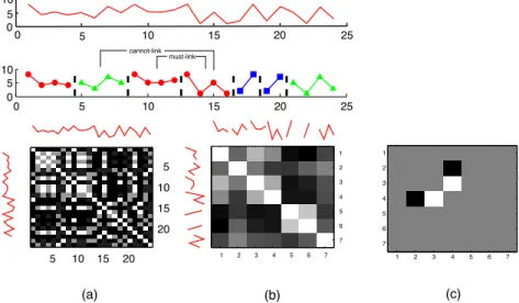
3.2 (a) shows the frame kernel matrix K, where each entry kij defines the simi-larity between two frames, xi and xj. (b) shows the segment kernel matrix calculated by DTAK. (c) shows the constraint matrix W. . . 31

3.3 Optimization of SSACA in a 1D sample. (a) Initial segmentation of sequence X into m subsequences s. The cannot-link constraint assists the segments X[sj,sj+1) andX[sj+2,sj+3). (b) Search process using forward phase and back-ward phase applied to every step of the optimization. The table keeps track of the head position i∗ v, the label gv∗, and the J(v) with the lowest values. (c) Converged segmentation. . . 34

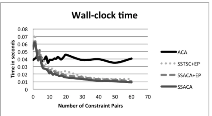
3.4 Wall time of the proposed semi-supervised methods compared to a com-pletely unsupervised method. . . 37

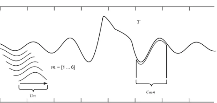
3.5 Sample time series T of length n, a subsequence in position m+i, and the first 6 subsequences extracted by a sliding window. Figure based on [2]. . . 43

3.6 Samples of the three different patterns (Cylinder, Bell, and Funnel) of the CBF dataset. . . 43

3.7 Cluster centers of the CBF dataset generated by kernelk-means. The shapes are similar to approximations of the original pattern. . . 44

(13)

3.8 Cluster centers of the CBF dataset generated by sliding windows using kernel

k-means. The shapes of the centers look like sine waves. . . 44

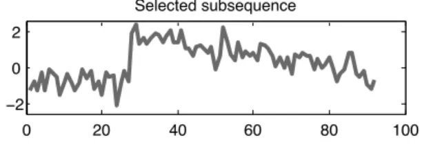
3.9 Retrieved subsequence generated by ACA. This sample is similar to the

Funnel pattern of the CBF dataset. . . 45

4.1 A sample time series from the synthetic dataset. . . 50

4.2 A sample of a time series with one pair of constraint. . . 52

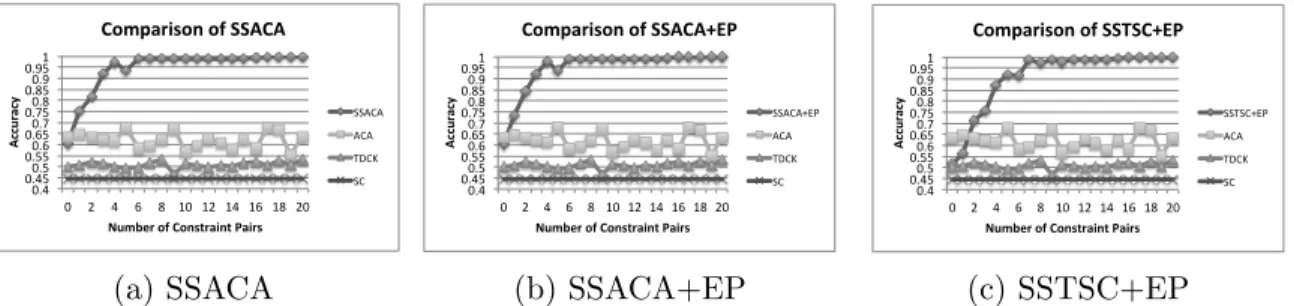
4.3 Constraint analysis of SSACA, SSACA+EP, SSTSC+EP. (a) Accuracy

av-erage, (b) Mean cluster variance, (c) Objective function values. . . 53

4.4 Comparison of SSACA, SSACA+EP, SSTSC+EP with ACA, SC, and TDCK.

. . . 54

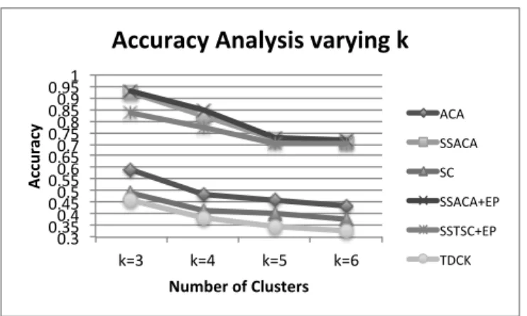
4.5 Analysis of variation of the number of clusters applied to a synthetic dataset. 56

4.6 Analysis of the effect of exhaustive propagation. . . 56

4.7 Comparison between the accuracy of only using the initial constrained seg-mentation and the accuracy of SSACA plus the initial constrained

segmen-tation. . . 58

4.8 Comparison between the accuracy of only using the initial constrained mentation and the accuracy of SSACA+EP plus the initial constrained

seg-mentation. . . 59

4.9 Comparison between the accuracy of only using the initial constrained mentation and the accuracy of SSTSC+EP plus the initial constrained

seg-mentation. . . 59

4.10 Comparison between the accuracy of only using the initial constrained seg-mentation and the accuracy of SSACA (initial constrained segseg-mentation +

similarity manipulations). . . 60

4.11 Comparison between the accuracy of only using the initial constrained seg-mentation and the accuracy of SSACA+EP (initial constrained

segmenta-tion + similarity manipulasegmenta-tions). . . 60

4.12 Comparison between the accuracy of only using the initial constrained seg-mentation and the accuracy of SSTSC+EP (initial constrained segseg-mentation

+ similarity manipulations). . . 61

5.1 The arousal-valance (A-V) space proposed by Russell with some plotted

(14)

5.2 Sample images from the VAM-Corpus dataset. . . 70

5.3 Discretization of the arousal dimensional emotion in subject 17 of VAM-Corpus dataset. . . 71

5.4 Accuracy of the analyzed methods compared to the ground truth of speaker 17 of VAM dataset. . . 73

5.5 Sample images of AVEC dataset. . . 74

5.6 Average accuracy results per subject for expectancy.. . . 74

5.7 Average accuracy results per subject for power. . . 75

5.8 Average accuracy results per subject for valence. . . 75

5.9 Average accuracy results per subject for arousal. . . 76

(15)

List of Abbreviations

ACA Aligned cluster analysis AU Action units

DP Dynamic programming

DPSearch Dynamic programming search DTAK Dynamic time alignment kernel DTW Dynamic time warping

EP Exhaustive propagation FACS Facial action coding system H Cluster alternation rate

HACA Hierarchical aligned cluster analysis HMRF Hidden Markov random fields LBP Local binary pattern

MCVar Mean cluster variance MOCAP Motion capture SC Spectral clustering

SSACA Semi-supervised aligned cluster analysis

SSACA+EP Semi-supervised aligned cluster analysis with exhaustive propagation SSDPSearch Semi-supervised dynamic programming search

SSTSC Semi-supervised temporal spectral clustering

SSTSC+EP Semi-supervised temporal spectral clustering with exhaustive propagation STS Subsequence time series

TC Temporal clustering

(16)

Chapter 1 Introduction

Clustering algorithms are known for their problem-solving applications when there is little a priori knowledge of the data being analyzed. For example, with a clustering problem, there is no need to know the classes beforehand. These are some well-known advantages of unsupervised methods in general. However, there are situations in which some limited knowledge of the data or application is available, and yet, there is no mechanism allowing the use of that knowledge in a clustering algorithm. Semi-supervised clustering is a strategy that incorporates limited supervision to guide the clustering process. This supervision is usually modelled by using class labels or constraints; as a result, some refer to this learning problem as “constrained clustering.”

By incorporating supervision into the clustering process, it is possible to improve ac-curacy and help the clustering algorithm in situations where the data is not well sep-arated. Some popular unsupervised algorithms that have been adapted into a semi-supervised framework are constrainedk-means clustering with background knowledge [3], semi-supervised kernel mean shift clustering [4], semi-supervised kernel k-means [5], and Constrained spectral clustering [6]. However, none of these methods are designed to handle temporal data.

Use of temporal data broadens the range of applications which can benefit from clus-tering. Traditional areas that incorporate temporal data and clustering are data mining, visualization, and segmentation. The problem of temporal clustering is the focus of this thesis, and is particularly important in applications such as human-motion analysis, audio-visual emotion analysis, and animal behaviour analysis. However, temporal clustering us-ing completely unsupervised methods may not produce satisfactory results. In some cases prior high-level knowledge may be known about the data, or some labeled data may be

(17)

available. This information can be used to aid the clustering algorithm. In this thesis, this problem is referred to semi-supervised temporal clustering, which can also be described as the combination of temporal and semi-supervised clustering.

1.1 Proposed Work

This thesis proposes an approach to creating semi-supervised methods which perform tem-poral clustering. This approach is exclusive to kernel-based clustering methods, and it is based on two concepts. First, it uses the idea of instance-level constraints, in the form of

must-link and cannot-link, as a way to add supervision to the clustering methods.

Sec-ond, it uses a dynamic-programming method, inspired by [7], to search for the optimal temporal clusters. The proposed approach was applied to two methods, namely, aligned cluster analysis (ACA) and spectral clustering (SC). To validate the advantage of the proposed temporal semi-supervised clustering methods, they were compared with their original versions and with another semi-supervised temporal cluster, using both synthetic and real-world data.

1.2 Summary of Contributions

The main contributions of this thesis can be summarized as follows:

• Proposal of semi-supervised aligned cluster analysis (SSACA), an extension of the temporal clustering method aligned cluster analysis (ACA).

• Proposal of semi-supervised temporal spectral clustering (SSTSC), an application of the dynamic programming search optimization proposed in [8] to the problem of constrained spectral clustering.

• Introduction of exhaustive propagation (EP) into the proposed methods to create SSACA+EP and SSTSC+EP, helping improving accuracy.

• Application of semi-supervised temporal clustering to spontaneous continuous emo-tion segmentaemo-tion.

(18)

1.3 Thesis Organization

This thesis is organized as follows.

Chapter 2gives an overview of the fundamentals necessary to understand the concepts of semi-supervised temporal clustering. Sections 2.1 and 2.2 explain, respectively, some time series representations and some similarity measures. Section2.3 discusses some of the main tasks in the field of time series. Section 2.4 describes time series segmentation and explains popular methods of carrying out segmentation. Section 2.5 gives an overview of clustering methods, and Section2.6 explains the kernel k-means clustering algorithm and other traditional algorithms. Section 2.7 introduces semi-supervised clustering and how constraints are used as supervision. Finally, Section 2.8 explains temporal clustering.

Chapter 3 introduces the proposed methods and offers some considerations about the use of constraints. Chapter 3 also provides a theoretical comparison with subsequence time series (STS). Section3.1derives the problem of temporal clustering, and Section3.2revisits the ACA method to give some background. Section 3.3 explains the process of adding supervision in the form of pairwise constraints to ACA, using the semi-supervised kernel

k-means framework. Sections 3.4 and 3.5 introduce the two proposed methods, SSACA and SSTSC, respectively. Section 3.6explains how an exhaustive constraint propagation is added to SSACA and SSTSC to create SSACA+EP and SSTSC+EP, which are explained in Sections3.7 and3.8, respectively. Finally, Sections3.9and3.10discuss some theoretical considerations related to the proposed methods.

Chapter 4 evaluates the performance of the proposed methods when applied to syn-thetic data. Section 4.1 presents the setup of the experiments and some quantitative and qualitative evaluation measures. Section 4.2 shows some comparative results of the pro-posed methods in a synthetic dataset and a complete analysis of how different variables can influence these methods.

Chapter 5 evaluates the performance of the proposed methods when applied to real-world applications. Before analyzing the results, this chapter gives an overview of the problem of emotion analysis and human motion segmentation. Section 5.1 introduces emotion analysis in the context of the visual modality, and how facial expression relates to emotion states. It also describes the fundamental steps required to develop an automatic facial expression recognition system, and differentiates the two most common ways to interpret emotion: categorical and dimensional models. Finally, Section5.1.2shows results of the comparison between the proposed methods and other related methods on the VAM Corpus dataset, and Section 5.1.5 shows results and comparisons on the AVEC emotion dataset. Section 5.2 discusses the problem of human motion segmentation and shows the

(19)

results of the comparisons between the proposed methods and other related methods when applied to a motion capture dataset.

Finally, Chapter6concludes the thesis, and discusses future extensions of this research, as well as additional applications that might benefit from the proposed methods. Also provided in this chapter is a list of publications produced by this research.

(20)

Chapter 2 Background and Literature Review

This chapter presents an overview of some fundamental concepts of temporal clustering and semi-supervised methods. The overview starts with some concepts of time series. Later, some background on clustering algorithms is discussed, with a particular emphasis on kernel-based methods, which are the focus of this thesis. This chapter also discusses the concept of semi-supervised clustering and how constraints can be used to aid the clustering process. The chapter closes with a review of related work.

2.1 Time Series Representation

According to [9], a time series is a collection of chronological observations. Representation of time series poses a fundamental problem, especially when the goal is to reduce their dimensionality of the time series. The simplest method of representing a time series is by sampling. Sampling involves selecting data representatives at fixed intervals, such that a more concise representation can be obtained. However, if the sampling rate is too low, this approach can result in distortions in the shape of the representation. An alternative method of representation is to use the average value of the data points within fixed-sized windows. This method is also known as piecewise aggregate approximation (PAA)[10]. Similar variations on this method have also been proposed, such as adaptive piecewise constant approximation (APCA)[11], in which the length of the window is adaptable, and piecewise linear representation (PLR).

Another type of time series representation involves transformation of the time series from the time domain to a different domain. Discrete Fourier transform (DFT) is a popular

(21)

transformation technique, first used by [12]. Discrete wavelet transform (DWT), Haar transform [13], and singular value decomposition (SVD) [14] offer alternative approaches to DFT.

Another family of representation consists of transforming numeric time series into a symbolic representations. SAX [15] is an example of this type of approach. This method first transform the data into a PAA representation, and then symbolizes the PAA into a discrete string. A benefit of this type of representation is its ability to produce distance measures that lower bounds the distance measures in the original series. In other words, SAX allows the use of various algorithms, such as clustering, classification, and anomaly detection, in the new representation, while still obtaining the same results.

2.2 Similarity Measures

Similarity measure plays a major role in solving many time series tasks. The most com-monly used distance measure for time series is the Euclidean distance, also known as

L2-norm. Given two time seriesT and Q of size n, the Euclidean distance is given by:

Dist(P, Q) = v u u t n X i=1 (pi−qi)2. (2.1)

[16] describes this family of distance aslock-step measures, which refer to all the distance measures comparing theith point of one time series to theith point of another time series. They also include the other Lp norms, such as L1-norm (city block distance); Linf-norm;

and DISSIM [17]. Another category of distance is called elastic measures, which include distance measures that allow for comparison of either one-to-many points or one-to-none (e.g., LCSS). Some of the distance measures which fall into this category are Longest Common SubSequence (LCSS) [18], Edit Sequence on Real Sequence, Swale, Edit Distance with Real Penalty (ERP) [19], and dynamic time warping (DTW) [20]. In contrast with

lock-step measures, which only compare time series of the same sizes,elastic measures have

the capability to measure time series of different sizes and handle local time shifting – i.e., time series that are similar, but are out of phase.

More recently, two other categories of similarity measures were proposed. The first of these categories is threshold-based measure, and the second is pattern-based measure. TQuEST [21] distance is an example of threshold-based distance. TQuEST transforms the time series into threshold-crossing time intervals, wherein the points within each time

(22)

interval have values greater than a threshold τ. Then, each interval is treated in a two-dimensional space, the first dimension being starting time, and the second being the ending time. Later, the similarity is defined as the Minkowski sum of the two sequences of time interval points. SpADe [22] is an example of pattern-based similarity measure, the second of the recent measures. SpADe attempts to detect matching segments within the entire time series by shifting and scaling in both temporal and amplitudinal dimensions. The similarity is represented by the set of matching pattern with the greatest degree of likeness.

2.2.1 Dynamic Time Warping

Dynamic time warping is one of the most frequently used measures in time series. This technique was proposed by [20] as an application for speech recognition. DTW allows for the measurement of similarities between temporal sequences which varies in time or speed, and can be computed by dynamic programming. Dynamic programming is a method for solving complex problems by recursively breaking them down into simpler subproblems. The complexity of DTW is O(n2_{); however, there are lower bound implementations with}

amortized complexities [23].

In order to align a sequenceP of lengthn, and a sequenceQ of lengthm using DTW, certain steps are necessary. The first step is to create a n-by-m matrix M, where the (ith_{, j}th_{) element of the matrix} _m

i,j is a squared distance (Euclidean distance) d(pi, qi) =

(pi −qi)2 corresponding with the alignment between points pi and qj. Second, in order

to find the best alignment between the two sequences, the algorithm must retrieve a path through the matrix that minimizes the total cumulative distance. The optimal path is the one that minimizes the warping cost

DT W(P, Q) = min    v u u t K X k=1 wk    , (2.2)

where wk is an element (i, j)k of the warping path W, which is a contiguous set of matrix

elements that defines a mapping between P andQ. Itskth _{element is defined as} _W

k(ik, jk)

and W =w1, w2, . . . , wk, . . . , wK, where max(m, n)≤K < m+n−1.

The warping path is subject to some constraint sets. The first constraint set is called boundary condition, and it requires that the warping start and finish diagonally. The second set of constraints is the continuity, meaning that if wk = (a, b), thenwk−1 = (a0, b0),

(23)

cells that are adjacent. The third constraint set only allows a₋a0 _≥ _{0 and} _b ₋_b0 _≥ _0,

which forces the points in W to be monotonically spaced in time.

The optimization can be executed by dynamic programming, in order to evaluate the following recurrence equation

γ(i, j) = d(pi, qj) +min{γ(i−1, j−1), γ(i−1, j), γ(i, j−1)}, (2.3)

whered(pi, qj) is the distance found in the current cell, andγ(i, j) is the cumulative distance

of d(i, j), and the minimum cumulative distance of the three adjacent cells. Although DTW creates a distance-like measure between time sequences, one drawback of using it as an approach is that it does not guarantee the triangle inequality property.

2.2.2 Dynamic Time Alignment Kernel (DTAK)

Dynamic time alignment kernel (DTAK) [24] is another technique that aligns time series, and offers a metric for calculating distances between them. DTAK is an extension of DTW; however, in contrast with DTW, DTAK satisfies the Cauchy-Schwartz inequality, and can also be solved efficiently by dynamic programming. Much like DTW, when given a sequence X = [x1, . . . , xnx] ∈ R

d×nx _{and a sequence} _Y _{= [}_y

1, . . . , yny] ∈ R

d×ny_{, DTAK}

creates a cumulative kernel matrix U _∈Rnx×ny which can be computed recursively by uij = max    u_i−1,j+kij ui−1,j−1+ 2kij ui,j−1+ki,j, (2.4) such thatu11= 2k11 wherekij =φ(xTi )φ(yj) = exp

−kxi−yjk2

2σ2

, which is the frame kernel matrix K_∈Rnx×ny. The distance between X and Y is given by

τ(X,Y) = unxny

nx+ny

. (2.5)

[25] points out one of the drawbacks of DTAK: it is not necessarily a strictly positive definite kernel, and a regularization of the kernel matrix therefore needs to be performed.

(24)

2.3 Time Series Tasks

Time series is widely studied in the field of data mining, and includes several related research areas, such as finding similar time series, subsequence searching in time series, dimensionality reduction, and segmentation.

A summary list of some of the main time series tasks includes [15]:

• Indexing: Consists of finding the most similar data series in a database, given a query time series P and a similarity measure.

• Clustering: Consists of organizing time series into similar groups, such that time series in the same group are more similar to each other than to those in other groups, given a similarity measure.

• Classification: Consists of assigning a given unlabelled time seriesP to a predefined class.

• Summarization: Consists of creating a smaller (possibly graphical) representation of a very large time series P, such that it retains its essential features.

• Anomaly Dectection: Consists of finding anomalies (unexpected, surprising, in-consistent) in the sections of a given time seriesP, given a model of “normal”behaviour.

• Segmentation: Consists of partitioning a given time serie P into k segments that are internally homogeneous [26].

2.4 Time Series Segmentation

A popular solution for segmentation in time series comes from solving the change detection problem. Change-point detection consists of an analysis of changes on the distribution of the points within a window of temporal observations, in order to locate their boundaries. The standard solution as [9] describes consists of fixing the number of change-points, then identifying their positions, and finally, determining functions for curve-fitting the intervals between successive change-points. A typical strategy for triggering a change-point is when the probability distributions of time series samples, over past and present intervals becomes significantly different [27] [28]. However, this technique detects only local boundaries, and does not provide a global model for temporal events.

(25)

Another group of methods uses non-parametric approaches, such as kernel density estimation, which are designed with no particular parametric assumptions. However, these estimations exhibit reduced accuracy in high-dimensional problems. According to [29], a recently-introduced strategy estimates the ratio of the probabilities directly without going through density estimation [30] (e.g., kernel mean matching [31], the logistic-regression method, and the Kullback-Leibler importance estimation procedure (KLIEP)), and has shown promising results.

Another popular way of performing time series segmentation is through a switching linear dynamic system (SLDS). Linear dynamical systems (LDSs) are useful in describing dynamical phenomena. However, such phenomena change over time, and as a result, the models that represent the phenomena also change. Switching several linear dynamic systems over time allows for description of the dynamics of the time series. The switching states in SLDS inference provide the segmentation of an input sequence implicitly. Because of the intractability of finding exact inferences, some approximations have been proposed: in [32], which casts the SLDS model as a dynamic Bayesian network; in [33], which presents a data-driven MCMC (DD-MCMC) sampling method for approximate inference in SLDSs; and [34], which uses a nonparametric Bayesian approach for learning switching dynamical processes by extending the HDP-HMM formulation.

Other approaches tackle segmentation from the perspective of analyzing periodicity of cyclic events [35] [36]. However, cyclic motion analysis only extracts segments of repeti-tive motion, which may leave some portion of the signal unsegmented and therefore not modelled.

Segmentation in video can be done by clustering frames and grouping those that are assigned to the same cluster to form a segment. One example of this technique is proposed by [37], which uses an action-based distance to group actions in a video by clustering similar frames. However, this approach performs segmentation as a later step of clustering; consequently it lacks a mechanism by which to incorporate the dynamics of the temporal events in the clustering process, as [38] indicates. Another method to segment time series involves obtaining segments that are internally homogeneous, and aim to minimize the overall cost of the segmentation. In other words, the optimalk-segmentation of time series

s using costing function CostF(s1s2. . . sk) is minimal among all possible k-segmentations

[39] [40]. This problem can be, however, stated as a clustering problem – if, for example the overall cost function is defined as the minimization of the distances of the centre of the clusters.

Some methods, however, attempt to solve the problem of segmentation as a global model for temporal events. These methods actually solve the problem by minimizing the

(26)

errors across various segments for eachk cluster, in order to find the segments. This subset of segmentation method relates to this thesis, and it is discussed in great detail in Section

2.8. First, however, some background on clustering algorithms must be given to further contextualize the challenges addressed by this type of approach.

2.5 Clustering

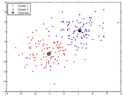
Data clustering is the main task of unsupervised learning. Unlike supervised methods, unlabelled data is used as the basis of learning: the data samples involved in the learning process have no categories previously assigned. Clustering consists of grouping data points into the same group, or “cluster,” as it is usually called, such that data points in the same cluster are more similar to each other (internal criterion) than to those in another cluster (external criterion). Figure2.1 depicts an example of a cluster.

−4 −3 −2 −1 0 1 2 3 4 −5 −4 −3 −2 −1 0 1 2 3 4 Cluster 1 Cluster 2 Centroids

Figure 2.1: 2D random points clustered by k-means algorithm. N

represent the centroid of each cluster.

(27)

2.5.1 Clustering Objective Function

Consider a set_X ofnelementsx1, . . . , xnthat needs to be clustered inksubsetsC1, . . . ,Ck,

where elements in the same cluster are more similar to each other than the elements in a different cluster. In order to make this statement a well-defined problem, it is necessary to define an objective function that measures the quality of any partition of the data [41]. The challenge subsequently becomes a matter of finding the partitions that optimize the objective function.

One simple way of defining an objective function for clustering is to use the sum-of-squared-error. Let ni be the number of samples in Ci, and let µi be the mean of those

samples defined by µi = 1 ni N X x∈Ci x. (2.6)

The sum-of-squared errors is defined by

Jc = k X i=1 X x∈Ci kx₋µik2. (2.7)

For a given cluster _Ci , the mean vector µi is the best representative of samples Xi,

since it minimizes the sum of the squared lengths of the error vectors x−µi in the subset Ci. Therefore, Jc is the total squared error incurred to represent the n samplesx1, . . . , xn

by the k centres µ1, . . . , µk. The optimal partition is the one that minimizes Jc, whose

value depends on how the samples are grouped into clusters and the number of clusters. This type of clustering is called minimum variance partition.

2.5.2 Similarity Measures

The clustering problem consists of finding a natural group of data that satisfies both an internal and external criterion. In order to define that samples in one cluster are more similar to one another than the samples in other clusters, a similarity measure must be defined. The most straightforward way to defining similarity or dissimilarity between two points is to use the distance between them. The distances most often used for a numerical datax, y _∈Rm are based on L2, L1 and L∞ norm.

(28)

L2 norm is the Euclidean, distance defined by d(x, y) = (( m X i=1 |xi−yi|2) 1 2), (2.8)

L1 norm, which is also known as city block metric, and is defined by

d(x, y) = (

m

X

i=1

|xi−yi|), (2.9)

and L∞ norm or Chebyshev distance, defined by

d(x, y) = max

i (|xi−yi|). (2.10)

A non-metric similarity function s(x, y) is another type of measurement that can be used is to compare the angular similarity of two vectors x and y. Conventionally, this function is symmetric and its value is large when x and y are similar in some way. The function can, for example, be used to measure the angle between vectorsx and y. In fact, this measurement is the cosine of the angle between them.

s(x, y) = x

t_y

kxkkyk (2.11)

Other types of similarity measurements are specific to categorical (nominal) data, in-cluding Hamming distance (the number of attributes taking different values) and edit distances. Yet, another class of similarity measures is based on kernels. Next section discusses the use of kernel as a similarity measurement.

2.5.3 Kernel as Similarity Measure

Let us denote a set of n objects by _S = (xi, . . . xn). Suppose that each object xi is an

element of a set_X, and therefore, a representationφ(x)_{∈ F} is defined for each object. In a classical representation the data set S is denoted as φ(S) = (φ(x1, . . . , φ(nn)). All the

methods explained above are based on this classical, individual representation of the data as feature vectors. However, there is a whole family of methods based on a set of pairwise comparisons. In other words, they are represented as real-valued comparison functions

(29)

k : _{X × X →} R, and the data set S is represented by the n × n matrix of pairwise

comparisons ki,j = k(xi, xj) [42]. This type of representation produces squared matrices,

which are completely independent of the nature of the objects being analyzed. As a result, data of different natures can be analyzed with this unified framework, which is part of a family of algorithms known as “kernel methods.”

2.6 Clustering Algorithms

Clustering algorithms are mainly categorized into partitional and hierarchical [1]. The choice of which type of algorithms to use depends on the nature of the data being analyzed and the prior knowledge available about the data. Figure 2.2 provides an overview of the main types of clustering algorithms. This subsection will briefly introduces these two categories.

2.6.1 Partitional Clustering

Partitioning algorithms, also known as “flat clustering”, divide data points into non-overlapping clusters in order to optimize a certain criterion function such as the one defined in Section 2.5.1. A standard algorithm that gives an effective representation of the parti-tioning category is thek-means algorithm. The goal of k-means is to group the data points into k partitions such that the distance between the points in each cluster and its centroid is minimized. Refer to Algorithm 1, which outlines the algorithm’s pseudocode.

The algorithm performs a greedy minimization of the criterion function; however, there is no guarantee of reaching a global minimum. The quality of the obtained solution depends on the initial partitioning of the data points. An heuristic for obtaining a better (albeit not optimal) solution is to repeat the algorithm, starting from different initial solutions, and to return the solution with the minimum value of the criterion function.

Another partitioning algorithm is called k-medoids. K-medoids is a variation of k -means, which instead of using the mean point to define the centre of the clusters, it uses actual points to represent the cluster. As a result, this method is more robust to noises and outliers. K-medoids determines the k centres, which are actual points, by minimizing the sum of the distances between each point and the nearest centre. The Partitioning around Medoids (PAM) is a method that implements this approach, and its time complexity is

O(K(N₋K)2_I_{), where}_N _{is the number of points,}_K _{is the number of clusters, and}_I _the

(30)

Clustering Algorithms Hierarchical Agglomera3ve Single Link Complete Link Divisive Par33onal Distribu3on/ density Mixture models DBScan Squared-‐error k-‐means Kernel k-‐ means Graph theore3c Spectral MST Nearest neighbor 1 to k-‐NN

Figure 2.2: Taxonomy of clustering algorithms. [1]

Kernel Clustering

As discussed in Section2.5.3, there is a family of methods (kernel methods) that use square matrices that are symmetric-positive-definite. In other words, if k is an n×n matrix of pairwise comparisons, it should satisfy ki,j = kj,i for any 1 ≤ i, j ≤ n, and c>kc ≥ 0 for

any c_∈Rn_{, as described in [}₄₂_{]. This family of methods includes approaches such as SVM}

[44], PCA, kernelk-means [45], Spectral Clustering [46], non-negative matrix factorization (NMF) [47], and kernel Self-Organizing Maps [48].

Kernelk-means is one of the simplest kernel clustering algorithms, and is a non-linear extension of the k-means. In kernel k-means, the Euclidean distance function is simply replaced by a non-linear distance function, which has the capacity of projecting the data into higher dimensions.

(31)

Algorithm 1 k-means

1: Choose randomly k points centres C1,...,Ck. 2: while the clusters are changing do

3: Reassign the data points. 4: for i= 1→n do

5: Assign data point xi to the cluster whose centreCj is closest 6: end for

7: end while

8: Update the cluster centrers. 9: for j= 1→k do 10: nj = number of points in C_j; 11: cj = _n1 j P xi∈Cjxi 12: end for

intok disjoint groups by minimizing the within-cluster variation. It finds the partition of the data that is a local optimum of the following energy function:

Jkkm(G) = k X c=1 n X i=1 gcikφ(xi)−zck2 | {z } dist2 φ(xi,zc) =_kX₋ZG_k2_F, s.t.GT1k = 1n, _(2.12)

where xi ∈ Rd (see notation1.) is a vector representing the ith data point, φ(.) is a

nonlinear mapping function, and zc ∈ Rd represents the centroid of the data points in

cluster c. Matrix G _{∈ {}0,1_}k×n _{indicates, in a binary format, the cluster to which} _x i

belongs, and Z∈Rd×n is the actual value of the means.

The squared distance between theith element and the centre of the clustercrepresented bydist2

φ(xi,zc) can be calculated as:

dist2φ(xi,zc) =ki,i− 2 nc n X j=1 gcjkij + 1 n2 c n X j1,j2=1 gcj1gcj2kj1j2, (2.13)

wherenc=Pnj=1gcj represents the total number of samples that are in cluster c, and the

kernel functionk is given bykij =φ(xi)Tφ(xj).

(32)

Kernelk-means follows the same approach as regulark-means, and assigns a data point

xi to the cluster whose mean ˙z, which was computed in the previous step, it is closest to,

that is gc∗ i = 1, wherec ∗ i = arg min c dist2_φ(xi,˙zc). (2.14)

The algorithm subsequently updates the new cluster centres. Although kernelk-means cannot explicitly compute the centres, there is no need to do so, because the distances

dist2

φ(xi,˙zc) between the samples and the means can be retrieved from the kernel matrix.

2.6.2 Hierarchical Clustering

Hierarchical algorithms construct the clusters by building a nested structure or tree, also known as dendrogram (Figure 2.3). The root of the tree represents the top cluster, and the leaf nodes represent the singleton clusters.

1 7 2 4 3 5 6 0.2 0.3 0.4 0.5 0.6 0.7 0.8 0.9 1 Similarity Figure 2.3: Dendrogram

Unlike partitioning algorithms, hierarchical clustering does not require the number of clusters to be specified. However, a flat-partition can be obtained by traversing the root

(33)

of the dendrogram until a number of clusters arise. A flat-partition can also be acquired by defining a threshold of the combination similarity between clusters and cutting off the tree at this specific point.

The strategy for construction of the tree can be generated in two ways: agglomerative hierarchical clustering (AHC) or divisive hierarchical clustering (DHC). AHC begins with singleton clusters, and then merges the most similar pairs of clusters until all data is grouped in one cluster. DHC operates in the opposite direction, with all the data points as one cluster, and then a partition of the dissimilar groups into separate clusters until each point becomes a singleton.

Of the two approaches AHC is more commonly used in applications ostensibly because the DHC criterion is less natural and more computationally expensive. Instances of AHC differ in their methods of calculating the similarities and distances between pairs of clusters. The most common methods are:

1. Single-link clustering: The distance between two clusters is computed as the distance between the two closest elements in the two clusters.

d(Ci, Cj) = min{d(xi, xj)|∀xi ∈Ci,∀xj ∈Cj (2.15)

2. Complete-link clustering: The distance between two clusters is computed as the maximum distance between the farthest elements in two clusters.

d(Ci, Cj) = max{d(xi, xj)|∀xi ∈Ci,∀xj ∈Cj (2.16)

3. Average-link clustering: The distance between two clusters is computed as the average distance between objects from the first cluster and objects from the second cluster. d(Ci, Cj) = 1 |Ci| × |Cj| X xi∈Ci xj∈Cj d(xi, xj) (2.17)

The dendrogram that is generated using the hierarchical algorithm displays the struc-ture of the data distribution. This type of strucstruc-ture allows for the number of clusters to be chosen a posterior, unlike from k-means and k-median, which require a priori number of clusters.

(34)

Hierarchical clustering algorithms possess some limitations. AHC follows a greedy pro-cess in order to decide whether to merge or split clusters. The decision, once made, is never reconsidered in later steps. Another limitation of AHC is its computational com-plexity (O(N3_{)) in the worst-case for computing pairwise similarities and iterations.}

AHC includes many other approaches beyond those described above. Some of these alternatives use hybrid algorithms, such as BIRCH (Balanced Iterative Reducing and Clustering using Hierarchies) [49], to address the aforementioned limitations. Other al-gorithms include CURE (Clustering Using REpresentatives), ROCK (RObust Clustering using linKs), CHAMELEON, and SOTM (Self-organizing Hierarchical Variance Map) [50].

2.7 Semi-Supervised Clustering

In machine learning, unsupervised methods such as clustering algorithms have been used in a variety of tasks, though mainly in exploratory data analysis. Some examples of these tasks include group discovery, data compression, dimensionality reduction, and outlier detection. In some certain tasks, some expert knowledge may be available, such as labels, relationship between data, or global assumption that are part of the domains. The process of leveraging extra knowledge is known as “semi-supervised learning”. Semi-supervised learning exists at the intersection between supervised and unsupervised learning, and falls into two categories:

1. Semi-supervised classification: Tasks falling into this category are, essentially, supervised in the presence of low quantities of supervision. Semi-supervised classi-fication uses the addition of unlabelled data to help supervised classifier learning. Semi-supervised classification nevertheless suffers from the same limitations as other supervised methods, including a priori knowledge of the number of classes and a minimum number of training samples for each class.

2. Semi-supervised clustering: Also known as constrained clustering, semi-supervised clustering is essentially an unsupervised method that uses the addition of some super-vision to support the clustering process. Classes are not known beforehand; therefore, there is no need for a minimum number of data samples for each class.

The reason why semi-supervised clustering is also known as “constrained clustering” is because constraints are the typical approach to leveraging supervision in the clustering

(35)

process. These constraints usually come in pairs, and are commonly known as “pairwise constraints.”

Methods such Constrained K-means Clustering with Background Knowledge represent a category of semi-supervised clustering algorithms. COP-KMEANS, as the authors of [3] call their algorithm, is a modification of the popular k-means algorithm that uses instance-level constraints in the form of must-link andcannot-link constraints. During the assignment phase of k-means, in which points are assigned to the closest clusters, COP-KMEANS ensures that no constraint is broken, guiding the clustering process towards a more appropriate partitioning of the data.

Basu et al. [51] propose a probabilistic model for semi-supervised clustering, based on Hidden Markov random fields (HMRFs). Their model is a combination of a constraint-based method, which uses constraints to modify the objective function, and a distance-based method, which trains similarities to satisfy constraints. This method partitions the data into k clusters, such that the total distortion between the points and the representa-tives of the clusters is minimized, and a minimum number of constraints are violated in the process.

Anand et al. [4] propose a kernel mean shift algorithm that incorporates pairwise constraints. Their method first maps the data to a high-dimensional kernel space. Then, by using a linear transformation, the points are projected to a space where the constraints are enforced. The authors show that this transformation can be achieved implicitly by modifying the kernel matrix. This method is another effort directed towards transforming an established clustering algorithm into semi-supervised clustering.

2.7.1 Pairwise Constraints

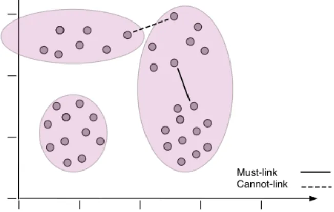
The use of extra knowledge in the clustering process can be of great value for improving accuracy, or even for creating clusters with desirable geometric properties [52]. One way of incorporating this extra knowledge is through the introduction of constraints. Constraints can be introduced at the cluster level (group of instances), in ways such as constraining the size of a cluster [53], constraining neighbours in a cluster to be within a certain threshold distance [54], or forcing time contiguity of instances in a temporal clustering [55]. Con-straints can also be introduced at the instance level. The most common instance-level constraints are must-link and cannot-link [56]. A must-link constraint denotes that two instances x and y must be in the same cluster, whereas a cannot-link constraint denotes that two instancex and y must not be in the same cluster. Figure 2.4 illustrates the con-cept of must-links and cannot-links. In many situations where there is no domain expert

(36)

available, feedback in the form of these two constraints is easier to acquire, compared to the actual label. Since must-link constraints share symmetrical, reflexive, and transitive properties, it can be inferred that, if (x, y)_{∈ M} and (y, z)_{∈ M ⇒}(x, z)_{∈ M}, where_M represents a set of must-links. Therefore, it is possible to infer extra pairs of constraints by applying transitive closure.

Must-link Cannot-link

Figure 2.4: Pairwise constraints in the form of must-link and cannot-link

The use of pairwise constraints can also contribute to seeding the cluster initialization. For example, during cluster initialization, points that are must-links should start in the same cluster, whereas points that are cannot-links should start in different clusters.

2.8 Temporal Clustering

Temporal clustering (TC) can be defined as the partitioning of multiple time series into a set of non-overlapping segments that belong to k temporal clusters [38]. Temporal clus-tering is similar to normal clusclus-tering in that both require a similarity measures, clusclus-tering algorithms, and evaluation criteria; however, the temporal nature of the data requires spe-cial treatment when it comes to one or more of these components. The two major ways of handling time series are either to modify existing static data-clustering algorithms to handle time, or to convert the time series into a form that works with static algorithms. The former approach relies, in most cases, on modifying the similarity measure to an ap-propriate measure of time series, such as DTW and DTAK. The latter maps the time series into a different representation or domain that embeds the temporal information – such as Wavelets, Fourier, and Haar transform [9] – or into a number of model parameters, and then applies the conventional static data clustering algorithm.

(37)

Temporal clustering can be used as a tool to solve segmentation problems. Applying a clustering approach to the segmentation problem requires global modelling of all temporal segments in a time series, instead of only finding local boundaries. As a result, simply using some of the traditional time series segmentation techniques, such as change point detection, may not produce satisfactory results. HACA [25] and ACA [7] solve this problem by minimizing errors across various segments for eachk cluster, yet, all of these methods lack mechanisms for adding supervision.

Most of the time series clustering techniques, such as the ones reviewed in [57], assume that the time series are already segmented, which underlies the main difference between the traditional time series clustering techniques and TC.

2.9 Related Work

Semi-supervised temporal clustering, as its name suggests, combines temporal and semi-supervised clustering in order to perform temporal segmentation. Much like general clus-tering approaches, temporal segmentation using clusclus-tering may not produce satisfactory results, due to being a completely unsupervised approach. In some situations, however, prior high-level knowledge exists about the segments, or some labeled data is available. This information can be used to aid the clustering algorithm.

However, there are few methods discussed in the literature dealing with both temporal and semi-supervised aspects. Of the few methods available, temporal-driven constrainedk -means (TDCK) [55] shows the best results compared to other methods such as TCK-means [58], Constrained k-means, and Temporal-Driven k-means, as described in [59]. TDCK offers a framework to model external information and add it to an unsupervised algorithm. Originally created as a solution to the problem of detecting typical evolution patterns, such as country evolutions, TDCK also provides benefits to applications for social network analysis, such as detecting social roles. Intuitively, TDCK adds must-links between all the pairs of observations belonging to the same entity. This mechanism, however, restricts the method to lower control at the instance level, and does not allow the use of cannot-links.

[60] describes a similar method, which combines discriminative cluster analysis (DCA) with a temporal and a semi-supervised term. The paper describes a semi-supervised tempo-ral clustering algorithm used to group large amounts of multimodal data into different ac-tivities. Similar to the approach used in [55], the constraints penalize non-smooth changes (over time) on the assigned clusters. However, there is no control over the granularity of the temporal term, and there is also no robust metric between time series.

(38)

2.9.1 Temporal-Driven Constrained K-means

The goal of TDCK is to cluster observations xi ∈ X, which are descriptions of entities

at a given timestamp written as triples (entity, timestamp, description): xi = (xφi, xti, xdi),

where xd

i ∈ D is the vector in the multidimensional description space that describes the

entityxi ∈Φ in time xti ∈ T, while taking into account both the temporal component and

the multidimensional description [59]. TDCK-means searches to minimize the following objective function: X µj∈M X xi∈Cj      kxi−µjkT A+ X xk∈C|/ xφ_k=xφ_i w(xi, xk)      , (2.18)

where k·kT A is a temporal dissimilarity measure, w(xi, xj) is the cost function that

de-termines the penalty of clustering adjacent observations of the same entity into different clusters, andCj is the set of observations in cluster j.

The temporally-aware dissimilarity measure combines distances, both in the multidi-mensional space_D and in the time space_T, and is described as follows:

kxi−xjkT A= 1− 1−γd kxd i −xdjk2 ∆x2 max ! × 1₋γtk xt i −xtjk2 ∆t2 max , (2.19)

where γd is the weight given to the multidimensional component of the temporally-aware

dissimilarity measure, and γt is the weight of the temporal component. The cost function

w(xi, xj) encourages temporally-adjacent observations that belong to the same entity to

be assigned to the same cluster. The cost function is defined as:

w(xi, xj) =β×e −12 _k xti−_xtjk δ 2 1[xφ_i =xφ_j] (2.20) [59] compares TDCK to other methods available in the literature – such as TCK-means [58], Constrained k-means, Temporal-Driven k-means – and proves it to be the most effective approach to temporal clustering.

(39)

Chapter 3 Proposed Semi-Supervised Temporal

Clustering

The problem addressed in this research is different from simple clustering of time series, which refers to the problem of clustering time series when they are already segmented. More specifically, it is a temporal clustering problem, which is explained in Section3.1. The main goal of this chapter is to explain the process of adding side information to a temporal clustering algorithm. The approaches proposed in this chapter are an extension of aligned cluster analysis (ACA), a temporal-clustering method, which is described in Section 3.2. The particular mechanism of which side information is added to the clustering method is based on the semi-supervised kernel k-means framework, which is explained in Section

3.3. Sections3.4 and 3.5detail the two proposed methods, semi-supervised aligned cluster analysis (SSACA) and semi-supervised temporal spectral clustering (SSTSC), and Section

3.6 discusses a constraint-propagation mechanism used to extend SSACA and SSTSC. The extended methods are discussed in Sections 3.7and 3.8. Finally, Section3.9 elaborates on the use of constraints on semi-supervised methods, and Section3.10explains the differences between the proposed methods and subsequence time series (STS).

3.1 The Problem of Temporal Clustering

Given a time series X = [x1, . . . , xn] ∈ Rd×n, find a vector s ∈ Rm that contains the

start positions ofm segments, wherem is the total number of segments, and each segment

A Semi-Supervised Approach for Kernel-Based Temporal Clustering