Modelling and Tracking of the Global Maximum Power Point in Shaded Solar PV Systems Using Computational Intelligence

i

Modelling and Tracking of the

Global Maximum Power Point in

Shaded Solar PV Systems Using

Computational Intelligence

Prepared by:

Arnold Farai Sagonda

SGNARN002

Department of Electrical Engineering University of Cape Town

Prepared for:

Prof. Komla Folly

Department of Electrical Engineering University of Cape Town

January 2019

Submitted to the Department of Electrical Engineering at the University of Cape Town Dissertation presented for the degree of Master of Science in Engineering

University

of

Cape

The copyright of this thesis vests in the author. No

quotation from it or information derived from it is to be

published without full acknowledgement of the source.

The thesis is to be used for private study or

non-commercial research purposes only.

Published by the University of Cape Town (UCT) in terms

of the non-exclusive license granted to UCT by the author.

University

of

Cape

ii

Declaration 1-Plagiarism

I, Arnold Farai Sagonda, hereby declare that the work on which this dissertation is based on is my original work (except where acknowledgements indicate otherwise) and that neither the whole work nor any part of it has been, is being, or is to be submitted for another degree in this or any other university. I authorise the University to reproduce for the purpose of research either the whole or any portion of the contents in any manner whatsoever.

Name: Sagonda Arnold Farai

iii

Declaration 2-Publications

DETAILS OF CONTRIBUTION TO PUBLICATIONS: Publications:

A.F. Sagonda, K.A. Folly. “Modelling and electrical output power assessment of a solar PV system”: A review, SAUPEC 2017

A.F. Sagonda, K.A. Folly, “Comparison of three Techniques for Maximum Power Tracking of solar PV systems”, IEEE World Congress on Computation Intelligence (WCCI) 2018.

Name: Sagonda Arnold Farai

iv

Acknowledgements

I would like to take this opportunity to thank my supervisor Professor Komla Folly for not only your guidance and assistance but also for your passion and drive for excellence, which I have adopted. Professor Folly, I am indebted to you for the support you have given me as your student, for the confidence you showed in my abilities.

Special thanks is owed to Kenneth Ainah, my friend, for such a high achiever thank you for making me realise that I can be ‘more powerful’.

Thanks to all my fellow peers for making this experience very fruitful.

Finally, to my parents I am very grateful for your unequivocal faith in me, your guidance and support, which have made it possible for me to achieve this.

v

ABSTRACT

Solar Photovoltaic (PV) systems are renewable energy sources that are environmentally friendly and are now widely used as a source of power generation. The power produced by solar PV varies with temperature, solar irradiance and load. This variation is nonlinear and it is difficult to predict how much power will be produced by the solar PV system. When the solar panel is directly coupled to the load, the power delivered is not optimal unless the load is properly matched to the PV system. In the case of a matched load the variation of irradiance and temperature will change this matching so a maximum peak power point tracking is therefore necessary for maximum efficiency.

The complete PV system with a maximum power point tracking (MPPT) includes the solar panel array, MPPT algorithm and a DC-DC converter topology. Each subsystem is modelled and simulated in MATLAB/Simulink environment. The components are then combined with a DC resistive load to assess the overall performance when the PV panels are subjected to different weather conditions. The PV panel is modelled based on the Shockley diode equation and is used to predict the electrical characteristic curves under different irradiances and temperatures.

In this dissertation, five MPPT algorithms were investigated. These algorithms include the standard Perturb and Observe (PnO), Incremental conductance (IC), Fuzzy Logic (FL), Particle Swarm Optimisation (PSO) and the Firefly Optimisation (FA). The algorithms are tested under different weather conditions including partial shading. The Particle Swarm and Firefly algorithm performed relatively the same and were chosen to be the best under all test conditions as they were the most efficient and were able to track the global maximum power point under partial shading. The PnO and IC performed well under static and varying irradiance, the PnO was seen to lose track of the MPP under rapid increasing irradiance. The PnO was tested under partial shaded conditions and it was seen that it is not reliable under these conditions. The Fuzzy logic performed better than the PnO and IC but was not as good as the PSO and FA. Since the fuzzy logic requires extensive tuning to converge it was not tested under partial shaded conditions.

A DC-DC boost converter interface study between a DC source and the DC load are performed. This includes the steady state and dynamic analysis of the Boost converter. The converter is linearised about its steady state operating point and the transfer function is obtained using the state space averaged model.

The simulation results of the complete PV system show that PSO and Firefly algorithm provided the best results under all weather conditions compared to other algorithms. They provided less oscillations at steady state, high efficiency in tracking (99%), quick convergence time at maximum power point and where able to track global power under partial shaded weather conditions for all partial shaded patterns. The Fuzzy logic performed well for what it was tested for which are static irradiance and rapid varying irradiance.

vi

The PnO and IC also performed relatively well but showed a lot of ringing at steady state. The PnO failed to track the MPP at certain instances under rapid increasing irradiance and the IC was shown to be unstable at low irradiance. The PnO was not reliable in tracking the global maximum power point under partial shaded conditions as it converged at local maximum power points for some partial shaded patterns.

vii

Table of Contents

Chapter 1: Introduction ... 15

1.1 Background ... 15

1.2 Motivation ... 15

1.3 Scope and Limitations ... 16

1.4 Dissertation outline... 16

1.5 Contributions ... 17

Chapter 2: Literature Review ... 18

2.1 Photovoltaic Modules, Strings and Arrays... 18

2.1.1 The semiconductor p-n junction diode ... 18

2.1.2 The Solar cell ... 18

2.1.3 Basic model of a solar cell ... 19

2.1.4 General model of a solar cell ... 20

2.1.5 PV module and array ... 24

2.2 Characteristics Curves of PV... 26

2.2.1 I-V Characteristics ... 26

2.2.2 Fill factor (FF) ... 26

2.2.3 The effects of temperature ... 26

2.2.4 The effects of irradiation ... 27

2.2.5 Solar I-V characteristics with resistive load ... 28

2.3 Effects of partial shading ... 28

2.3.1 Partial shading and bypass diode effects ... 29

2.3.2 Characteristic curves under partial shading ... 29

2.3.3 Mitigation methods for partial shading ... 30

2.4 DC-DC Boost Converter ... 31

2.5 Summary ... 33

Chapter 3: Optimisation basics ... 35

3.1 Optimisation techniques ... 35

3.1.1 Deterministic algorithms ... 35

3.1.2 Stochastic Algorithms ... 35

3.1.3 Optimisation classifications ... 36

3.2 Summary ... 36

Chapter 4. Maximum power point tracking and DC-DC Boost converter control ... 38

4.1 Photovoltaic maximum power point tracking ... 38

4.1.1 Performance specifications of MPPT control algorithm ... 39

4.1.1.1 Steady-state error ... 39

4.1.1.2 Dynamic response ... 39

4.1.1.3 Tracking efficiency ... 39

4.2 MPPT algorithms ... 40

4.2.1 Perturb and Observe ... 40

4.2.2 Incremental Conductance ... 42

4.2.3 Load matching with the PV array ... 44

4.2.4 Constant voltage technique (CV) ... 44

viii

4.2.6 Fuzzy Logic MPPT controller ... 46

4.2.6.1 Fuzzification ... 48

4.2.6.2 Defuzzification ... 49

4.2.7 Unique GMPP ... 50

4.2.8 Metaheuristic algorithms in MPPT ... 51

4.3 Control of the Boost Converter ... 51

4.3.1 State space averaging technique ... 52

4.3.1.1 Small signal of the boost converter ... 54

4.3.2 Controller design ... 57

4.4 Summary ... 58

Chapter 5: Particle Swarm Optimisation and The Firefly algorithm ... 59

5.1 The Firefly algorithm ... 59

5.1.1 Concept ... 59

5.1.2 Light intensity and attractiveness ... 59

5.1.3 Algorithm parameters ... 61

5.1.4 Firefly algorithm in MPPT in PV systems ... 61

5.2 Particle Swarm Optimization ... 65

5.2.1 Algorithm parameters ... 66

5.2.2 PSO algorithm for MPPT in PV systems ... 67

5.3 Summary ... 69

Chapter 6: Simulation Results ... 70

6.1 System design... 70

6.2 PV modelling and validation at STC... 71

6.3 Boost Converter Design and Control ... 77

6.4 MPPT using conventional algorithms and metaheuristic algorithms ... 83

6.4.1 Principle of load matching according to the system design ... 84

6.4.2 Algorithm efficiency at static atmospheric conditions ... 85

6.4.3 Performance of the five algorithms under rapid varying irradiance ... 93

6.4.4 The effects of the step size for the PnO algorithm ... 98

6.4.5 Partial shading conditions ... 100

6.5 Summary ...114

Chapter 7 Conclusion and Recommendations... 115

7.1 Conclusion ...115

7.2 Recommendation ...116

List of References ... 117

Appendices ... 123

Appendix A: Actual Data sheet of PV module parameter ...123

Appendix B: Mathematical modelling of the PV module ...124

Appendix C: m-file Code for boost converter small signal model and control ...126

Appendix D: Direct connection of PV system with a matched load ...128

Appendix E: Fuzzy Logic ...129

Appendix F: Results of MPPT of the algorithms for 800,600 and 500 W/m2 ...131

Appendix G: Voltage and Current for varying irradiance ...134

Appendix H: I-V Partial shading patterns ...136

ix

List of Figures

FIGURE 2. 1: SYMBOL OF A P-N JUNCTION DIODE ... 18

FIGURE 2. 2: THE PHYSICS OF A P-N JUNCTION SEMICONDUCTOR... 18

FIGURE 2. 3: A SOLAR CELL CONNECTED TO A LOAD AND THE FLOW OF CURRENT ... 19

FIGURE 2. 4: BASIC PV CELL MODEL ... 19

FIGURE 2. 5: GENERAL MODEL MOSTLY USED IN PV CELL ... 21

FIGURE 2. 6: THE EFFECTS OF RSH ON THE I-V CHARACTERISTIC CURVE ... 21

FIGURE 2.7:THE EFFECTS OF RSH ON THE P-V CHARACTERISTIC CURVE ... 22

FIGURE 2.8:THE EFFECTS OF RS ON THE I-V CHARACTERISTIC CURVE... 22

FIGURE 2.9:THE EFFECTS OF RS ON THE P-V CHARACTERISTIC CURVE... 23

FIGURE 2.10:ITERATIVE PROCESS OF FINDING RSH AND RS ... 24

FIGURE 2. 11: SOLAR CELLS INTERCONNECTED TO FORM A MODULE ... 25

FIGURE 2. 12: MODULES INTERCONNECTED TO FOAM A PV ARRAY ... 25

FIGURE 2. 13: I-V CHARACTERISTIC CURVE SHOWING FILL FACTOR ... 26

FIGURE 2. 14:THE EFFECTS OF TEMPERATURE ON THE PHOTOVOLTAIC I-V AND P-V CHARACTERISTIC ... 27

FIGURE 2. 15:THE EFFECTS OF IRRADIANCE ON THE PHOTOVOLTAIC I-V AND P-V CHARACTERISTIC ... 27

FIGURE 2. 16: THE INTECSECTION OF THE RESISTIVE LOAD CURVE WITH THE PHOTOVOLTAIC I-V CURVE ... 28

FIGURE 2. 17: CONNECTION OF BYPASS DIODE ACROSS THE MODULE ... 29

FIGURE 2. 18: I-V AND P-V CHARACTERISTICS UNDER PARTIAL SHADING ... 30

FIGURE 2. 19: I-V AND P-V CHARACTERISTICS UNDER PSC SHOWING LOCAL POWER AND GLOBAL ... 30

FIGURE 2. 20:DC-DC BOOST CONVERTER ... 31

FIGURE 2. 21:HOW THE VOLTAGE AND INDUCTOR CURRENT BEHAVES IN CONTINUOUS CURRENT MODE. ... 32

FIGURE 2. 22: EQUIVALENT CIRCUIT FOR BOOST CONVERTER (A) SWITCH ON; (B) SWITCH OFF . ... 32

FIGURE 3. 1: OPTIMISATION CLASSIFICATIONS ... 37

FIGURE 4. 1: BLOCK DIAGRAM OF A MPPT FOR PV SYSTEMS ... 39

FIGURE 4. 2: HOW THE PNO OPERATES ON THE PHOTOVOLTAIC P-V CURVE ... 40

FIGURE 4. 3:FLOW CHART OF THE PNO ALGORITHM ... 41

FIGURE 4. 4: DIVERGENCE OF THE PNO METHOD DURING A RAPIDLY CHANGING IRRADIANCE LEVEL ... 42

FIGURE 4. 5:INCREMENTAL CONDUCTANCE METHOD ON THE P-V CURVE OF A SOLAR MODULE ... 43

FIGURE 4. 6:THE FLOW CHART OF THE INCREMENTAL CONDUCTANCE ... 44

FIGURE 4. 7: VOLTAGE CONTROL METHOD FOR MPPT WITH FIXED VOLTAGE REFERENCE ... 45

FIGURE 4. 8: FLOWCHART FOR FRACTIONAL SHORT-CIRCUIT CURRENT ALGORITHM ... 46

FIGURE 4. 9:VARIOUS SHAPES OF MEMBERSHIP FUNCTIONS (A) MONOTONIC (B) TRAPEZOIDAL (C) TRIANGULAR (D) GAUSSIAN ... 47

FIGURE 4. 10: THE FUZZY CONTROLLER DIAGRAM ... 47

FIGURE 4. 11: MEMBERSHIP FUNCTIONS OF E, E AND D ... 48

FIGURE 4. 12: CENTER OF GRAVITY METHOD EXAMPLE ... 49

FIGURE 4. 13: CENTER OF GRAVITY METHOD EXAMPLE FOR DISCRETE MEMBERSHIP FUNCTION ... 50

FIGURE 4. 14: UNIQUE GLOBAL POWER MAXIMUM STRATEGY ... 50

FIGURE 4. 15: VOLTAGE CONTROL OF A DC-DC CONVERTER ... 52

FIGURE 4. 16: A TYPICAL RESPONSE TO A SECOND ORDER SYSTEM ... 57

FIGURE 4. 17: CONTROLLER SETUP ... 58

FIGURE 5. 1: TRAJECTORY MOVEMENTS OF FIREFLY 1 ... 61

FIGURE 5. 2: THE VOLTAGE CONTROL METHOD ... 62

FIGURE 5. 3: FIREFLY FLOW CHART FOR MPPT ... 64

FIGURE 5. 4: MOVEMENT OF PARTICLES IN THE OPTIMISATION PROCESS ... 65

x

FIGURE 6. 1:COMPLETE PV SYSTEM ... 70

FIGURE 6. 2:THE BUILT PV MODULE... 71

FIGURE 6. 3: P-V CURVE OF VARIATION OF RS WITH RSH CONSTANT ... 72

FIGURE 6. 4: I-V CURVE OF VARIATION OF RS WITH RSH CONSTANT ... 72

FIGURE 6. 5:P-V CURVE VARYING RSH WITH RS CONSTANT (A) THE WHOLE P-V CURVE (B) ZOOMED AT MPP ... 73

FIGURE 6. 6:I-V CURVE VARYING RSH WITH RS CONSTANT ... 74

FIGURE 6. 7:P-V CURVE SHOWING VARIATION IN TEMPRETURE WITH IRRADIENCE CONSTANT ... 75

FIGURE 6. 8:I-V CURVE OF VARIATION OF TEMPRETURE WITH IRRADIENCE CONSTANT ... 75

FIGURE 6. 9:P-V CURVE OF VARIATION IN IRRADIENCE WITH TEMPRETURE CONSTANT ... 76

FIGURE 6. 10:I-V CURVE OF VARIATION IN IRRADIENCE WITH TEMPRETURE CONSTANT ... 76

FIGURE 6. 11:BOOST CONVERTER ... 77

FIGURE 6. 12: BOOST CONVETER OUTPUT VOLTAGE ... 78

FIGURE 6. 13: ZOOMED BOOST CONVETER OUTPUT VOLTAGE ... 78

FIGURE 6. 14: ROOT LOCUS OF THE BOOST CONVERTER ... 79

FIGURE 6. 15:CLOSED LOOP CONTROL OF THE BOOST CONVETER ... 79

FIGURE 6. 16:PI PARAMETERS FOUND USING THE SISOTOOL ... 80

FIGURE 6. 17:CLOSED LOOP ROOT LOCUS EDITOR OF THE BOOST TRANSFER FUNCTION IN SISO TOOL. ... 80

FIGURE 6. 18:COROSPONDING STEP RESPONSE OF THE TRANSFER FUNCTION IN SISOTOOL... 81

FIGURE 6. 19:CLOSED LOOP SYSTEM OF THE BOOST CONVERTER ... 82

FIGURE 6. 20: PI CONTROLLER PERFORMANCE WITH A REFRENCE OF 200V ... 82

FIGURE 6. 21:PI CONTROLLER PERFORMANCE WITH STEP REFRENCES ... 83

FIGURE 6. 22: CONNECTION OF THE BOOST CONVERTER WITH THE SOLAR ARRAY ... 84

FIGURE 6. 23: EXTRACTED PV POWER UNDER AN IRRADIENCE OF 1000 W/M2 BY THE PNO AND IC ... 87

FIGURE 6. 24: PV VOLTAGE AT STC... 87

FIGURE 6. 25: PV CURRENT AT STC ... 88

FIGURE 6. 26: EXTRACTED PV POWER UNDER AN IRRADIANCE OF 1000 W/M2 BY THE PSO, FA AND FUZZY ... 89

FIGURE 6. 27: PV VOLTAGE AT STC FOR THE PSO, FA AND FUZZY ... 90

FIGURE 6. 28: PV CURRENT AT STC ... 91

FIGURE 6. 29: CONVERGENCY SPEED OF ALGORTHMS AT STC ... 92

FIGURE 6. 30:SEARCH PROCESS OF THE FA IN FINDING BEST VOLTAGE (VREF) ... 92

FIGURE 6. 31:VARYING IRRADIENCE PROFILE ... 94

FIGURE 6. 32: MPP TRACKING BY THE PNO AND IC CONTROLLERS AT DIFFERENT CHANGES IN WEATHER CONDITIONS ... 96

FIGURE 6. 33: MPP TRACKING BY THE PSO, FA AND FUZZY CONTROLLERS AT DIFFERENT CHANGES IN WEATHER CONDITIONS ... 98

FIGURE 6. 34: EFFECTS OF DIFFERENT STEP SIZE FOR THE PNO UNDER STC ... 99

FIGURE 6. 35: CONVERGENCY SPEED OF THE DIFFERENT STEP SIZE ... 100

FIGURE 6. 36: P-V CURVE OF PATTERN 1 ... 101

FIGURE 6. 37:PV POWER TRACKED BY THE PSO AND FA ... 102

FIGURE 6. 38: MPPT OF THE PV POWER FOR PATTERN1 BY THE PNO ... 103

FIGURE 6. 39: P-V CURVE PATTERN 2 ... 103

FIGURE 6. 40: PSO AND FA CONVERGING CLOSE TO GMPP... 104

FIGURE 6. 41:EXPLORATION PROCESS OF FIREFLIES TO FIND BEST VREF ... 105

FIGURE 6. 42:PNO CONVERGING AT GMPP ... 106

FIGURE 6. 43: P-V CURVE OF PATTERN 3 ... 106

FIGURE 6. 44: PSO AND FA CONVERGING CLOSE TO THE GMPP ... 107

FIGURE 6. 45: PNO CONVERGING AT LMP 3 ... 108

FIGURE 6. 46: PATTERN 4 ... 109

FIGURE 6. 47:PSO AND FA CONVERGING CLOSE TO GMPP ... 110

FIGURE 6. 48: PNO CONVERGING AT LMP 4 ... 110

xi

FIGURE 6. 50: PSO AND FA CONVERGING CLOSE TO GMPP... 112

FIGURE 6. 51: POWER TRACKED BY THE PNO ... 112

FIGURE A. 1 DATA SHEET OF ACTUAL PV MODULE ... 123

FIGURE A. 2 MATLAB SIMULINK PV MODULE BLOCK PARAMETERS ... 124

FIGURE B. 1 DETAILED IPH IMPLEMENTATION ... 124

FIGURE B. 2 DETAILED REFERENCE REVERSE SATURATION CURRENT ... 125

FIGURE B. 3 DETAILED SATURATION CURRENT VARYING WITH TEMPERATURE ... 125

FIGURE B. 4 DETAILED PV CURRENT WITH RS AND RSH ... 126

FIGURE C. 1 CLOSED LOOP STEP RESPONSE WITH OBTAINED PI PARAMETERS ... 127

FIGURE D. 1 MODEL OF DIRECT CONNECTION TO MATCHED LOAD IN SIMULINK ... 128

FIGURE D. 2 POWER RESULTS WITH MATCHED LOAD ... 129

FIGURE E. 1 FUZZY LOGIC SETUP ... 130

FIGURE F. 1 MPPT REULTS FOR STATIC IRRADIENCE OF 800 W/M2 ... 131

FIGURE F. 2 MPPT RESULTS FOR STATIC IRRADIENCE AT 600 W/M2 ... 132

FIGURE F. 3 POWER RESULTS FOR STATIC IRRADIENCE OF 500 W/M2 ... 133

FIGURE G. 1 VOLTAGE FOR VARYING IRRADIENCE ... 134

FIGURE G. 2 CURRENT FOR VAYING IRRADIENCE ... 135

FIGURE H. 1 I-V CURVE OF PATTERN 1 ... 136

FIGURE H. 2 I-V CURVE OF PATTERN 2 ... 136

FIGURE H. 3 I-V CUREVE FOR PATTERN 3 ... 137

FIGURE H. 4 I-V CUREVE FOR PATTERN 4 ... 137

FIGURE H. 5 I-V CUREVE FOR PATTERN 5 ... 138

FIGURE I. 1 PV VOLTAGE FOR PATTERN `1 ... 139

FIGURE I. 2 PV VOLTAGE FOR PATTERN 2 ... 140

FIGURE I. 3 PV VOLTAGE FOR PATTERN 3 ... 141

FIGURE I. 4 PV VOLTAGE FOR PATTERN 4 ... 142

FIGURE I. 5 PV VOLTAGE FOR PATTERN 5 ... 142

List of Tables

TABLE 4. 2: FUZZY LOGIC CONTROL RULE TABLE ... 49

TABLE 4. 3:EFFECTS OF CONTROLLER PARAMETERS ... 57

TABLE 5. 1:TERMINOLOGIES IN FA AND PV SYSTEM ... 62

TABLE 6. 1:SIMULINK BUILT IN PV MODULE PARAMETERS ... 71

TABLE 6. 2:PV STRING OF 5 MODULES IN SERIES ... 74

TABLE 6. 3:BOOST CONVERTER SPECIFICATION ... 77

TABLE 6. 4:BOOST CONERTER PARAMETERS ... 77

TABLE 6. 5:OPTIMISATION ALGORITHM PARAMETERS ... 85

TABLE 6. 6:PERFORMANCE OF THE ALGORTHMS AT DIFFERENT STATIC IRRADIENCE ... 93

TABLE 6. 7:IRRADIENCES EXPOSED TO EACH MODULE ... 101

xii

List of Abbreviations

AC Alternating Current AI Artificial Intelligence

CCM Continuous Conduction Mode CoG Centre of gravity

CI Computational Intelligence CV Constant Voltage

DC Direct Current

DPGS Distributed Power Generation System FA Firefly Algorithm

FF Fill Factor FL Fuzzy Logic

FLC Fuzzy Logic Controller

GMPP Global Maximum Power Point HC Hill Climbing

IC Incremental Conductance I-V Current-Voltage

KCL Kirchhoff Current Law KL Kirchhoff’s Laws KVL Kirchhoff Voltage Law LMPP Local Maximum Power Point MPP Maximum Power Point

MPPT Maximum Power Point Tracking P n O Perturb and Observe

PI Proportional Integral

PID Proportional Integral Derivative PSC Partial Shading Conditions PSO Particle Swarm Optimisation PV Photovoltaic

P-V Power-Voltage

PWM Pulse Width Modulation SC Short Circuit Current SISO Single- input Single –output STC Standard Test Conditions ZN Ziegler and Nichols

xiii

List of Symbols

C Capacitor D Duty ratio d Diode

𝐸𝑔𝑎𝑝 Semiconductor band-gap energy 𝑓𝑠 Switching frequency of Dc-dc Converter G Photovoltaic radiation

𝐺𝑟 Reference photovoltaic radiation 𝐼𝑀𝑃𝑃 Maximum power point current 𝐼_𝑜 Converter output current 𝐼_𝑝ℎ Photocurrent

𝐼𝑃𝑉 Photovoltaic current

𝐼𝑅𝑆 Reverse saturation current of solar cell 𝐼𝑆 Photovoltaic cell reverse saturation current 𝐼_𝑆𝐶 Photovoltaic model short-circuit current 𝐼_{𝑆𝐶,𝑟𝑒𝑓} Reference condition short-circuit current k Boltzmann’s constant

𝑁𝑝 Number of connected solar cells in parallel 𝑁_𝑠 Number of connected solar cells in series

𝑃_{𝑎𝑐𝑡𝑢𝑎𝑙} The real measured power produced by the PV array 𝑃𝑖𝑛 Input power of the converter

𝑃𝑚𝑎𝑥 Maximum power point

𝑃𝑜𝑢𝑡 Output power of the converter q The charge of electron

𝑅_𝑜𝑝𝑡 Resistive load optimum operating point 𝑅𝑆 Solar cell series resistance

𝑅𝑆ℎ Solar cell shunt resistance S Switch

T Operating temperature of solar cell

𝑇_𝐶 Operating temperature in kelvin for solar cell 𝑡_𝑜𝑓𝑓 Converter switch off duration

𝑡𝑜𝑛 Converter switch on duration 𝑇_𝑅𝑒𝑓 Reference temperature of solar cell

𝑇𝑆 Switching period of DC-DC converter 𝑉𝑑 DC-DC converter input voltage 𝑉𝐿 Voltage of the inductor

𝑉𝑚𝑎𝑥 Solar cell maximum power voltage 𝑉_𝑜 Output voltage of the converter 𝑉_𝑂𝐶 Solar model open-circuit voltage 𝛥𝑖𝐿 Value of inductor current ripple 𝑅𝑙𝑜𝑎𝑑 Resistance of load

xiv

𝑉𝑟𝑒𝑓 Reference voltage (usually equal to Vmpp) 𝑉𝑀𝑃𝑃 Voltage at Maximum Power Point

𝑐1 Cognitive component 𝑐2 Social component w Inertia weight

𝑝_{𝑏𝑒𝑠𝑡 ,𝑖} Personal best of agent 𝐺𝑏𝑒𝑠𝑡 Global best of swarm

𝑟𝑎𝑛𝑑1,2 Random number between 0 and 1 𝛼 The randomization parameter

𝛾 Variation of the attractiveness 𝛽 Firefly attractiveness

𝐼 Light intensity Iter current iteration

15

Chapter 1: Introduction

In this dissertation an investigation was done to determine the drawbacks of conventional algorithms (if any) for MPPT and how computational intelligent optimisation algorithms can be used to cope with these drawbacks. All the components involved in designing the complete system were investigated and discussed. This includes the static and dynamic behaviour of DC-DC converters, modelling of the PV cell using the single diode model. The unique condition of partial shading was investigated to understand how it alters the PV power –voltage characteristic curve.

1.1 Background

The traditional means of power generation through fossil fuel driven plants has since received severe criticism as it has unsolicited environmental effects on the atmosphere. The use of renewable energy has thus been motivated as a result.

Research on renewable and distributed energy sources is ongoing at accelerated rates all over the world. Photovoltaic (PV), wind and biomass are the most common and successful renewable energy sources currently in use. Grid-connected renewable energy sources like solar energy system uses power electronics converters to step up DC voltages, the renewable energy sources are often tied to the grid allowing power transfer from the inverter to the distribution grid. The interconnection between these small generation systems with the grid has since grown into a network called the Distributed Power Generation System (DPGS). Through the DPGS, renewable energy has since played a pivotal role in today’s energy scenario. Photovoltaic (PV), wind and biomass have continuously been developed and have shown that they are reliable and cost competitive [1]. The cost of these renewable energy sources is currently decreasing, and further decreases are expected with the increase in demand and improvement of production [2]. Many countries have adopted new energy policies to encourage investments in renewable energy sources. Solar energy can be harvested by means of photovoltaic cells. The major drawback of solar energy is that it is not available all the time and also the solar plants sometimes experience cloud cover problems.

1.2

Motivation

Large Solar plants and residential PV installations are becoming a major source of power generation in South Africa and worldwide. Various methods have been proposed in the literature on how to deal with the partial shading that can occur due to clouds and the mutual shading that occurs between adjacent PV blocks in solar plants. In residential PV installations, partial shading is even common due to buildings, trees, clouds, etc. The main method that exists to deal with partial shading is hardware fixture [3]. This approach is complex and expensive [3]. A simple and inexpensive way to deal with partial shaded conditions is therefore needed. Under partial shaded conditions, the PV power vs voltage characteristic curve has multiple power peaks. Computational intelligent (CI) control algorithms can be used to track the global maximum power point (GMPP). These algorithms provide a cheap method in dealing with partial shading conditions and are less complicated.

The major drawbacks of conventional optimisation algorithms such as PnO and IC are that they cannot distinguish between a global maximum power point (GMPP) and a local maximum power point (LMPP) under partial shading conditions. If the algorithm converges at a LMPP this results in power loss.

16

1.3

Scope and Limitations

This research is based on using computational intelligence as a tool for maximum power point tracking in PV systems. Optimisation using computational intelligence (CI) requires knowledge of identifying the function to optimise and the number of variables available.

The work covered in this dissertation includes, understanding maximum power point in PV systems and why it’s necessary. The converter selected will be the non-isolated boost converter, other non-isolated or isolated converters will not be covered in this work.

Precisely, the work in this research covers the application of the Particle swarm optimisation, Firefly algorithm and Fuzzy logic to MPPT control in PV systems. Validation of the CI algorithms is done by comparing them with widely used conventional algorithms.

1.4

Dissertation outline

Chapter 2

Provides a literature review of how the photovoltaic cells convert solar radiation energy to electrical energy. The chapter also shows how these cells are interconnected to create PV modules and then these modules are combined to build PV strings and PV arrays. An overview of the PV models used and the introduction of the functional principles and the electrical characteristic of the PV modules are presented. A review of how these PV modules are affected by the irradiance and temperature is presented. The Chapter also discusses partial shading and its effects on the solar PV output. The mitigation methods that exist to deal with partial shading are briefly discussed.

Chapter 3

A review of the relevant optimisation techniques is discussed. The different types of optimisation methods that exist i.e., deterministic and stochastic based optimisation are discussed. A brief review of examples of deterministic and stochastic based algorithms is undertaken showing the advantages and disadvantages of the techniques.

Chapter 4

Discussed the maximum power point techniques, the principle of maximum power transfer and load matching; the use of classical MPPT techniques is also discussed. The advantages and disadvantages of the conventional methods are explained. The chapter also provides a review of the use of computational intelligent algorithms in MPPT, and discusses their necessity under partial shading conditions. CI methods such as Fuzzy Logic (FL) are discussed. The dynamic behaviour of the converter selected is also studied based on the state space averaging technique.

17

This chapter introduces the Firefly (FA) optimisation algorithm based MPPT, the Particle swarm optimisation (PSO) algorithm. These Intelligent algorithms are discussed based on how they reduce oscillations at MPP, increase MPP extraction efficiency and increase tracing speed. It is shown that the PSO and FA are able to track the GMPP for any partial shading pattern.

Chapter 6

The implementation of the complete system in MATLAB/SIMULINK is described. This includes each of the subsystems in detail, the solar cell model, boost converter, dynamic behaviour of the boost converter with DC load and the proposed maximum power-point tracking methods. The MATLAB results of the maximum power point tracking methods applied in photovoltaic are also compared and discussed. Each MPPT method is investigated based on the performance criteria of convergence time, extracted power, and efficiency. The performance under different weather conditions and partial shading is also investigated.

Chapter 7

The chapter presents the conclusions and future work.

1.5 Contributions

The major contributions of the dissertation are

1. A clear illustration of the effect of starting point of deterministic algorithms in a multimodal objective function is illustrated. It is difficult to know where the GMPP will occur in partial shaded conditions hence it was shown that using gradient based algorithms under these conditions is not reliable.

2. The metaheuristic algorithms were shown to perform well for MPPT in PV systems than the PnO, IC and Fuzzy logic. The PSO and FA where able to find the GMPP under partial shading conditions where the deterministic algorithms failed.

18

Chapter 2: Literature Review

This chapter provides an explanation of solar cells, reviewing the relevant semiconductor physics of the solar cell and the general concept of how it converts solar irradiation into electricity. The effect of direct coupling a resistive load on the solar cell is also reviewed. The effects of partial shading are also discussed and how it is solved in the industry.

2.1

Photovoltaic Modules, Strings and Arrays

2.1.1 The semiconductor p-n junction diode

Figure 2.1 shows the electrical symbol of a diode [1].

Figure 2.1 Symbol of a p-n junction diode[1] 2.1.2 The Solar cell

Figure 2.2 shows the structure of the PV cell. The solar cell is made of a semiconductor of p-type and boron atoms to form the substrate. A p-n junction is created when a high-temperature diffusion process is used to add atoms of phosphorous to the substrate. Where the two semiconductors meet, the holes in the p region move into the n region, which leaves behind negative charge ions in the p-side. The electrons from the n-side move into the p-n-side leaving behind positive charged ions in the n-n-side. Due to the rearrangement of positively and negatively charged ions the depletion region shown in Figure 2.2 is created [1].

Figure 2.2:The physics of a p-n junction semiconductor[1]

Charge carriers are not found in the depletion region. Hole-electron pair charges will be constantly be created when the p-n material is exposed to solar radiation with enough photon energy. The electrons in

19

the p-n material will be excited because of the photon energy. If a semiconductor with n-type and p-type of a PV cell is connected to an external load as shown in Figure 2.3.

Figure 2.3: A solar cell connected to a load and the flow of current[1]

The electrons in the n-type semiconductor will move through the external load to combine with the holes in the p-type semiconductor. Figure 2.3 also shows how current is produced.

Mono-crystalline and poly-crystalline are the most used materials to make solar cells [1], [2], [3] . 2.1.3 Basic model of a solar cell

There are many different mathematical photovoltaic models that have been developed in the literature. The models are meant to give an estimation of how the PV cell would behave compared to the real cell. The accuracy of the model depends on how many internal variables are considered. A p-n junction diode connected across a current source is usually used to represent a basic solar cell. Figure 2.4 shows this model [4], [5] , [6].

Figure 2.4:Basic PV cell model [4]

In Figure. 2.4, 𝐷𝑗is the ideal p-n diode 𝐼𝑃𝑉 and 𝑉𝑃𝑉 are the PV cell current and voltage respectively.

The photocurrent produced by sunlight is represented by the current source. Applying the Kirchhoff current law to the model, the current-voltage characteristic function can be obtained as given in equation (2.1): 𝐼_𝑃𝑉= 𝐼_𝑃ℎ− 𝐼_𝐷 (2.1)

20

where 𝐼𝐷 is the current through the diode also known as internal diffusion current and 𝐼𝑃ℎ is the photon current which varies linearly with the sunlight radiation.

The diode internal diffusion current is represented by equation (2.2) below: 𝐼𝐷= 𝐼𝑆 [exp (

𝑞𝑉_𝑃𝑉

𝐴𝑘𝑇_𝐶) − 1] (2.2) where A is diode ideality factor usually between 1 and 2, k represents the Boltzmann’s constant which is 1.38 ⤬ 10−23 _{𝐽 𝐾⁄ , 𝑇}

𝐶 is the operating temperature of the cell in kelvin, the charge of an electron q is 1.6 × 10−19_{.The cell dark saturation current 𝐼}

𝑆 which changes with temperature is represented by equation (2.3) [7].

𝐼

= 𝐼

. (

)

_{. exp [}

(

−

)] (2.3)

where 𝐼𝑅𝑆 is the cell reverse saturation current in ampere at 𝑇𝑅𝑒𝑓 where 𝑇𝑅𝑒𝑓 is the solar cell reference temperature in kelvin, usually 298K (25°C). The band-gap energy of the semiconductor material is represented by 𝐸𝑔𝑎𝑝. Equation (2.4) represents the cells reverse saturation current at reference temperature [7].

𝐼_𝑅𝑆= 𝐼𝑆𝐶

exp ( 𝑞𝑉𝑜𝑐 𝐴𝑘𝑇𝑅𝑒𝑓) − 1

(2.4)

where 𝑉𝑂𝐶is the open-circuit voltage at reference temperature 𝑇𝑅𝑒𝑓. The photocurrent, 𝐼𝑃ℎ, is represented by equation (2.5).

𝐼_𝑃ℎ = [𝐼_𝑆𝐶+ 𝐾₁(𝑇_𝐶− 𝑇_𝑅𝑒𝑓)] 𝐺

𝐺_𝑟 (2.5) where 𝐼𝑆𝐶 is the short circuit current of the cell, 𝐾1 is the temperature coefficient of the cells short circuit in (amps/K), G is the solar radiation in 𝑊 𝑚⁄ 2 and 𝐺𝑟 represents the solar radiation reference, 𝐺𝑟 = 1𝑘𝑊 𝑚_⁄ 2_{. 𝐼}

𝑆𝐶 and 𝑉𝑂𝐶 are obtained under standard test condition (STC) at a reference temperature of 25 ° C and solar insolation of 1kW/m2 _{[4]- [6].}

2.1.4 General model of a solar cell

Figure 2.5 shows the general model that is mostly used in simulation software packages for prediction of solar production. It is more accurate than the model shown in Figure 2.4 this is because it includes the shunt resistance 𝑅𝑆ℎ and series resistance 𝑅𝑆.

21

Figure 2.5 General model mostly used in PV cell [5]

The PV cell output current 𝐼𝑃𝑉 in equation (2.1) becomes

𝐼_𝑃𝑉= 𝐼_𝑃ℎ− 𝐼_𝐷− 𝐼_𝑆ℎ (2.6) 𝐼𝑃𝑉= 𝐼𝑃ℎ− 𝐼𝑆[exp (𝑞(𝑉𝑃𝑉_𝐴𝑘𝑇+𝑅𝑆𝐼𝑃𝑉)

𝐶 ) − 1] − (

𝑉𝑃𝑉+𝑅𝑆.𝐼𝑃𝑉

𝑅𝑆ℎ ) (2.7)

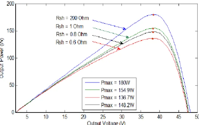
The p-n junction non-idealities and impurities near the junction which causes shunt leakage current to the ground are represented by the shunt resistance 𝑅𝑆ℎ. The bulk resistance of the semiconductor material is represented by 𝑅𝑆. The effects of of 𝑅𝑆ℎ on the PV characteristic curves are shown in Figure 2.6 and Figure 2.7, respectively. From Figure 2.7, it can be seen that the MPP ( 𝑃𝑚𝑎𝑥) i.e. the turning point of the curve, increases with the increase of RSh. The increase of RSh reaches a point where a further increase has no effect on the maximum power.

22

Figure 2.7: The effects of 𝑹𝑺𝒉 on the P-V characteristic curve[2]

A small variation on 𝑅𝑆 results in no change on the 𝐼𝑆𝐶 and the 𝑉𝑂𝐶 . The effects on the I-V and P-V characteristic curves are shown in Figure 2.8 and Figure 2.9, respectively [5] , [8]. From Figure 2.9 it can be seen that an increase in RS reduces the maximum power.

23

Figure 2.9: The effects of 𝑹𝑺 on the P-V characteristic curve[2]

To make the model more compelling and accurate 𝑅𝑆ℎ and 𝑅𝑆 are selected so that the calculated maximum power 𝑃𝑚𝑎𝑥 is equal to the experimental one 𝑃𝑚𝑎𝑥,𝑒𝑥𝑝 , at standard test conditions (STC) conditions seen on the module datasheet. Iterative processes are used to find the best values of 𝑅𝑆ℎ and 𝑅𝑆. There is only one pair of 𝑅𝑆 and 𝑅𝑆ℎ that will produce the required 𝑃𝑚𝑎𝑥. Iterative equations that can be used to find 𝑅𝑆ℎ are shown below [9].

𝐼_{𝑚𝑝,𝑟𝑒𝑓} =𝑃𝑚𝑝,𝑟𝑒𝑓 𝑉_{𝑚𝑝,𝑟𝑒𝑓} =

𝑃_{𝑚𝑎𝑥,𝑒𝑥𝑝}

𝑉_{𝑚𝑝,𝑟𝑒𝑓} (2.8) where 𝑉𝑚𝑝,𝑟𝑒𝑓 is maximum power voltage at STC.

𝐼_{𝑚𝑝,𝑟𝑒𝑓} = 𝐼_{𝑃ℎ,𝑟𝑒𝑓}− 𝐼_{𝑆,𝑟𝑒𝑓}[exp (𝑞(𝑉𝑚𝑝,𝑟𝑒𝑓_𝐴𝑘𝑇+ 𝑅𝑆𝐼𝑚𝑝,𝑟𝑒𝑓) 𝐶 ) − 1] − ( 𝑉_{𝑚𝑝,𝑟𝑒𝑓}+ 𝑅_𝑆. 𝐼_{𝑚𝑝,𝑟𝑒𝑓} 𝑅_𝑆ℎ ) (2.9) 𝑅_𝑆ℎ = 𝑉𝑚𝑝,𝑟𝑒𝑓+ 𝑅𝑆𝐼𝑚𝑝,𝑟𝑒𝑓 𝐼_{𝑠𝑐,𝑟𝑒𝑓}− 𝐼_{𝑠𝑐,𝑟𝑒𝑓}{exp [𝑉𝑚𝑝,𝑟𝑒𝑓+ 𝑅𝑠𝐼𝑚𝑝,𝑟𝑒𝑓_𝑎 − 𝑉𝑜𝑐,𝑟𝑒𝑓]]} + 𝐼_{𝑠𝑐,𝑟𝑒𝑓}{exp (−𝑉𝑜𝑐,𝑟𝑒𝑓_𝑎 )} − (𝑃_{𝑚𝑎𝑥,𝑒𝑥}/𝑉_{𝑚𝑝,𝑟𝑒𝑓}) (2.10) 𝑎 =𝑁𝑠𝐴𝑘𝑇𝑐 𝑞 (2.11) where 𝑁𝑠 is the number of solar cells connected in series. TC is temperature.

The iteration starts at 𝑅𝑆= 0 which must be increased in order to move the modelled MPP until it equates with the experimental MPP [9]. The corresponding 𝑅𝑆ℎ is then computed. Figure 2.10 shows the flow chart.

24

Figure 2.10 Iterative process of finding 𝑹𝑺𝒉 and 𝑹𝑺 [9]

2.1.5 PV module and array

Because the solar cell power is very small around 2W at 0.5V, the solar cells are connected in series and parallel so as to form a module to produce a desired output power and voltage.

25

Figure 2.11: Solar cells interconnected to form a module[6]

The same current flows in two or more PV modules connected in series and the total output voltage is the sum of each PV module voltage connected. Hence equation (2.7) can be written as shown in equation (2.12). The PV module current ads up for each module connected in parallel, and the output voltage across remains constant. 𝐼_𝑃𝑉=. 𝑁_𝑝𝐼_𝑃ℎ− 𝑁_𝑝𝐼_𝑆[exp (𝑞 (𝑉𝑃𝑉+ 𝑁_𝑆 𝑁_𝑃𝑅𝑆𝐼𝑃𝑉) 𝑁_𝑆𝐴𝑘𝑇_𝐶 ) − 1] − ( 𝑉_𝑃𝑉+𝑁𝑆 𝑁_𝑃𝑅𝑆. 𝐼𝑃𝑉 𝑁_𝑆 𝑁_𝑃𝑅𝑆ℎ ) (2.12)

where 𝑁𝑃 are cells in parallel and 𝑁𝑠 is the number of PV cells connected in series. If these PV modules are connected in series they form a string where the current in the string stays the same but the voltage is a multiple of the number of modules in the string. When the PV strings are connected in parallel they form a PV array in this case the current flowing in one string is a multiple of the number of strings in the array and the string voltage is the same as the array voltage.

26

2.2

Characteristics Curves of PV

2.2.1 I-V Characteristics

𝐼𝑆𝐶 and𝑉𝑂𝐶 describe the electrical performance of a PV cell. The point where the curve crosses the vertical axis is the short circuit current. It is considered as the maximum possible current in the circuit.

Open circuit voltage is the point where the curve intercepts with the horizontal axis. It is considered as the maximum possible output voltage the circuit can produce.

2.2.2 Fill factor (FF)

The ratio of output PV power at MPP to the power result from multiplying 𝑉𝑂𝐶 by 𝐼𝑆𝐶 is called the fill factor of the PV cell. Equation (2.13) shows this. The shape of the photovoltaic cell characteristic depends on these fill factor as shown in Figure 2.13. A high quality cell with low internal losses has a high fill factor [9]. Equation (2.13) can be further simplified to equation (2.14).

𝐹𝐹 =𝐼𝑀𝑃𝑃𝑉𝑀𝑃𝑃 𝐼_𝑆𝐶𝑉_𝑂𝐶 =

𝐴𝑟𝑒𝑎 𝐵

𝐴𝑟𝑒𝑎 𝐴 (2.13) 𝐼_𝑆𝐶𝑉_𝑂𝐶𝐹𝐹 = 𝐼_𝑀𝑃𝑃𝑉_𝑀𝑃𝑃= 𝑃_𝑚𝑎𝑥 (2.14)

where 𝐼𝑀𝑃𝑃 is the current at MPP and 𝑉𝑀𝑃𝑃 is the voltage at MPP. The fill factor depends on the material used and is always less than one. A better operation performance of the PV cell is experienced if the fill factor is closer to unity. The fill factor is affected by RSh and RS as shown in Figure 2.6 and Figure 2.8 [8].

Figure 2.13: I-V characteristic curve showing fill factor[8]

2.2.3 The effects of temperature

Temperature is one of the parameter that affects the output power of photovoltaic panels. Figure 2.14 shows the effect of temperature at constant irradiance.

27

Figure 2.14:The effects of temperature on the photovoltaic I-V and P-V characteristic [10]

As can be seen from Figure 2.14, temperature affects mostly the open circuit voltage. It is clear that an increase in temperature results in a decrease in PV output power and a decrease in temperature results in an increase in PV power [10].

2.2.4 The effects of irradiation

Irradiation is another parameter that affects PV output maximum power as shown in Figure 2.15. From Figure 2.15, it is clear that as the irradiance increases the short current increases. The increase in irradiance results in an increase of PV output power. The short circuit current depends totally on irradiance and it varies linearly with it [10].

28

The PV cell will function in two main operating characteristic regions these are the voltage source region and current source region. Figure 2.16 shows the locations of these regions.

Figure 2.16: The intecsection of the resistive load curve with the photovoltaic I-V curve[11]

When a constant resistive load (R) is coupled directly to a PV module terminals, the operating point of the connection will depend on where the intersection of the PV cell curve with the load curve occurs. This can be seen in Figure 2.16. The resistance load has a straight line characteristic with a slope,_𝑉𝐼 = 1 𝑅⁄ [11],[12]. The size of the resistive load determines the power transferred from the PV source. If the resistance of the load is small, the PV cell operates in the current source region AB of the characteristic curve. When a large load resistance is connected, the PV cell operates on the voltage source region CD of the characteristic curve [13].

It is clear that the operating point of the load might not be at Z which is the MPP of the PV array and furthermore as seen from Figure 2.14 and Figure 2.15, this maximum power point will constantly vary with environmental changes of temperature, solar irradiance and really gets complicated under partial shading were multiple points of maximum power will exist. This variation is nonlinear which makes the matching of the two characteristics even more difficult [12].

2.3

Effects of partial shading

It was seen that under a constant irradiance, only one maximum power point exists. In reality, the irradiance exposed on modules connected in an array rarely is the same. This can be due to cloud cover,

29

daily sun angle changes, shading from adjacent PV modules or trees and buildings [14]. Power is lost due to shading, current mismatch in a string and voltage mismatch between strings in parallel. When PV panels connected in series do not receive the same solar irradiance partial shading will occur [15].

2.3.1 Partial shading and the bypass diode effects

As mentioned previously current that flows in modules connected in a series is the same including those which are under a shade.The shaded cells can act as loads if they get reverse biased this will cause them to consume power produced from the fully irradiated cells. Problems like hot spot occur if the modules are not protected. A bypass diode is connected across each module to mitigate this problem.

During normal operation of the panels without shade, the bypassed diode is reverse biased and has high impedance. Under shaded conditions, the bypass diode across the shaded module terminal is in forward biased, therefore it conducts the current produced by the unshaded modules. Since the shaded modules are bypassed, multiple peaks on the P-Vcurve and multiple stairs on the I-Vcurve are exhibited. Figure 2.17 shows how the bypass diode is connected [15].

.

Figure 2.17: Connection of Bypass Diode across the module[15]

2.3.2 Characteristic curves under partial shading

The bypass diodes connection will change the uniform PV characteristics curves of the panel, resulting in multiple peaks [16], [17]. Figure 2.18 illustrates this point.

30

Figure 2.18: I-V and P-V characteristics under partial shading[15]

Figure 2.18 shows the different voltage values were the different power peaks will occur. It can be seen that the GMP occurs at low voltage ( V2). Figure 2.19 shows the GMP ocuring at a midium voltage on the P-V characteristic curve.

Figure 2.19: : I-V and P-V characteristics under PSC showing local power and global[15]

It can be observed that the P-V curve has multiple maximum power peaks [18]. The position of the GMPP on P-V curves is not fixed as illustrated in Figure 2.19 and Figure 2.18. From Figure 2.18 and Figure 2.19 it can be seen that the number of multiple power peaks is equal to the number of stairs on I-V characteristic. 2.3.3 Mitigation methods for partial shading

Two methods are generally used to mitigate the shading effect. The first is based on hardware fixtures [19], [20], [21] , [22] ; multilevel converter system [23], allowing each PV source connected in series to be

31

controlled separately to its MPP; and power electronic equalizers [24]. This approach is complex and costly [25] hence an alternative cheaper method has to be found.

The second approach is to track the global maximum power (GMP) by developing computational intelligence algorithms (CI), and this will be the focus of this dissertation. Computational intelligent algorithms have been suggested to solve the multiple power peak problem in solar PV systems. The multiple power peaks can be seen as a stochastic optimisation problem and global optimisation algorithm techniques can be used to find the global peak (best power).

2.4

DC-DC Boost Converter

The switch mode DC-DC converter is a critical component for MPPT system. It is responsible for maximum power transfer from the PV source to the load. It achieves this by regulating the PV input voltage and producing a controlled dc output voltage [26].

A direct connection of a PV panel with a resistive load will result in the load operating where the characteristics of the curves intersect, this could be the MPP or not. The converters ensure that the PV array is forced to operate at the MPP. MPPT algorithms are used to control the duty cycle. This control of the duty cycle allows the curves to be matched at MPP even with the nonlinearly changes of the PV array power due temperature and irradiance. Different loads will have their own unique characteristic curves [2]. They are two types of DC-DC converter topologies these are isolated and non-isolated converters. Isolated converters use a transformer to isolate the input from the output [27]. They are commonly used in switched mode power supply [27], [26]. Non-isolated converters are the boost and buck converters. In this dissertation, only the boost converter topology will be reviewed.

The boost converter output voltage is always more than the input voltage [26]. Figure 2.20 shows the circuit topology of the boost converter.

The boost converter consists of four elements. These are inductor, diode, capacitor, and the M0SFET. The Boost converter can be used as a switching-mode regulator. The regulation is usually accomplished by pulse width modulation technique (PWM). The converter is operated in continuous conduction mode. Figure 2.21 shows how the voltage and inductor current behaves in this mode [26].

𝑉𝑑_𝑡𝑜𝑛+ (𝑉𝑑 − 𝑉𝑜)_{𝑡𝑜𝑓𝑓}= 0 (2.15)

32

Figure 2.22 shows the two operating states of the boost converter [26].

Equation (2.15) can be evaluated to obtain the steady state equation (2.16) [26] 𝑉_𝑜 𝑉_𝑑= 𝑇_𝑠 𝑡_𝑜𝑛= 1 1 − 𝐷 (2.16) Where D is the duty cycle.

Figure 2.21 :How the voltage and inductor current behaves in continuous current mode [26].

Figure 2.22 Equivalent Circuit for boost converter (a) switch ON; (b) switch OFF [26].

33

Assuming no losses in the circuit, power input is the same as power output [26]. 𝑃_𝑑 = 𝑃𝑜 Therefore 𝑉𝑑𝐼𝑑= 𝑉0𝐼𝑜 This results in 𝐼𝑜 𝐼 𝑑= (1 − 𝐷) (2.17) Equation (2.18) express the duty ratio D when the boost converter is at a stable state

𝐷 = 1 −𝑉𝑑

𝑉𝑜 (2.18)

where 𝑉𝑑 represents input voltage and 𝑉𝑜 output voltages of the converter. The filter inductor and capacitor can be calculated using equations (2.19) and (2.20).

𝐶𝑜𝑢𝑡 ≥

𝐼_𝑜𝑢𝑡𝐷

𝑓_𝑠𝑤∆𝑉_𝑜𝑢𝑡 (2.19) 𝐿_{𝑐𝑟𝑖𝑡𝑖𝑐𝑎𝑙}≥ 𝑉𝑖𝑛𝐷

𝑓_𝑠𝑤∆𝐼_𝐿 (2.20) where 𝑓𝑠𝑤 is the switching frequency, ∆𝐼𝐿 is the input current ripples and ∆𝑉𝑜𝑢𝑡 is the voltage output ripple

2.5

Summary

This chapter reviews the physical structure of solar cells and explains how electricity is produced when the semiconductor device is exposed to solar radiation. The voltage produced by the solar cell is very small therefore a need to connect the PV cells in a series configuration is required.

The chapter also presents two commonly used PV models for simulation prediction, the single diode model with series resistance and shut resistance and a single diode model without. The single diode model with series resistance and shut resistance is found to be more accurate to represent the actual solar cell and it is the one that is used in this dissertation. The series and shut resistance parameters of the single diode model have to be correctly found to accurately model the actual PV cell. These parameters can be found by iterative methods.

The chapter also discusses how temperature, radiation and the load type used affect the PV power produced. In the literature, it is found that an increase in temperature reduces the PV output power and a decrease in temperature increases PV output power. The increases in radiation increases the PV output power and the decreases of radiation decreases the PV power. The intersection of the characteristic curve of the load and the characteristic curve of the PV current - voltage is where the PV cell will operate. The constant variation of PV power due to changing climatic conditions makes the load matching difficult as a result a MPPT algorithm is needed to constantly extract the maximum power.

Constant radiation or temperature results in one maximum power point on the PV power-voltage characteristic curve but different illumination of radiation on different PV modules connected in series results in multiple maximum power points (partial shading). A bypass diode is connected across each

34

module to prevent hot spots. Mitigation methods are discussed to reduce the effect of partial shading and it was found that most of them are complex and expensive to implement. It is suggested that using computational intelligence algorithms to extract the optimum power from a partial shaded PV array can be less complex and yet still be effective. A review of the DC-DC boost converter is discussed as a critical component in MPPT. The converter is used to match the PV source with the load.

35

Chapter 3: Optimisation basics

In this chapter a review of relevant literature of optimisation techniques is presented. This includes the deterministic and stochastic optimisation methods. Advantages and disadvantages of these techniques are also discussed.

3.1

Optimisation techniques

Optimization is used in multiple fields from engineering design, computer science etc. . . . The need to maximize or minimize something is always necessary [28]. Optimization is basically searching for the best variables in a function so as to have the best outcome. Thus a problem can only be optimized if it can be expressed mathematically. The decision variables can be either discrete, continuous or a mixture of the two. The search space is the area covered by the decision variables and the space formed by the cost function variables is called the solution space [28]. Optimisation can be done to find the maximum or minimum value of the function. There are two optimization techniques which are classified as deterministic approach and stochastic approach.

3.1.1 Deterministic algorithms

Deterministic algorithms use one solution at a time, which will trace out a path as the iterations continue [29]. Good examples of deterministic approaches are the Hill-Climbing and the Perturb and Observe method. If the algorithm is made to start at the same starting point it will repeat the same path regardless of whether the code is run today or another time. Most conventional algorithms are deterministic [29]. Some deterministic optimization algorithms that use the gradient information are called gradient-based algorithms. An example is the Newton Raphson algorithm it uses the function derivatives to find the optimum point. It works very well for continuous unimodal problems [28]. If the function is now multimodal (having multiple peaks), finding the optimum point might be difficult using gradient based algorithms. For objective functions which are multimodal such as a sine function, gradient based optimization methods are very sensitive to the starting point. If the starting point is far from the sought minimum or maximum, the algorithm will usually get stuck in a local minimum and/or simply fail [28]. Nonlinearity and multimodality are the main problems, which render most conventional methods such as the hill-climbing method inefficient and lead them to be stuck to local inferior solutions [29]. Another challenge that comes about using deterministic approaches is when the number of decision variables are large for example 50000, coupled to the non-linearity of the function it can be impractical to search the number of possible combinations of the different variables that will give the best output. In this case an algorithm that does not use the gradient is preferred. Non-gradient algorithms use the function values and avoid any use of its derivative [29]. Stochastic algorithms also known as heuristic and metaheuristic algorithms are gradient-free algorithms that are designed to deal with these types of problems [28].

3.1.2 Stochastic Algorithms

Stochastic algorithms always have some form of randomness. A good example are the Genetic algorithms (GAs). The solutions in the population will be different each time the program is run this is because the algorithm will use some foam of pseudo-random values. Though the final outcome of the search process may be similar [29], the movement traced by each individual will not be exactly repeatable. Metaheuristic algorithms are also stochastic by nature. Heuristic means to find or discover by trial and error [29]. Meta

36

means beyond or high level. All metaheuristic algorithms rely on a tradeoff of randomization and local search. Randomization allows the search process to be biased on the global scale instead of the local scale [29]. Therefore, almost all metaheuristic algorithms intend to be suitable for global search optimization. In complex optimization problems, quality solutions can be obtained in a reasonable duration of time, but there is no guarantee that the best solutions are obtained [28]. This allows us to find easily obtainable good solutions which are not necessarily the optimum solutions which still allow us to fix the problem. Among the quality solutions found it is assumed that some of them are nearly optimum. It will be difficult to search every possible solution or combination to a given complex problem; the aim is to obtain quality feasible solutions in an acceptable timeframe. Metaheuristic algorithms use two major principles to search in a given search space these are intensification and diversification [28]. Diversification means different multiple solutions will be created so as to explore the global scale. Intensification means to concentrate the search in a local region by analyzing the information that a current quality solution is located in this region [29]. The selection of the best solution ensures that the solutions will converge to the optimality, while the randomization of solutions prevents the solutions from being trapped at local optima and increases the diversity of the solutions [30]. The good combination of diversification and intensification will encourage the global best to be found.

Metaheuristic algorithms can be classified as population-based meaning that one has multiple agents looking for the optimum solution. Examples of metaheuristic algorithms include the Particle Swarm Optimisation (PSO), Firefly (FA), Bat (BA), Harmony search (HS), Cuckoo search (CS), Grey Wolf (GW), Ant Colony Optimisation (ACO), Flower Pollination (FP), etc. Alternatively, there is no universally better algorithms that exist. The main research goal in optimization is to come up with the most suitable and efficient algorithms for a given optimization problem. The complexity of the objective functions usually indicates the complexity of an optimization problem [28].

3.1.3 Optimisation classifications

The classification of optimisation problems based on the number of objectives will result in two categories: single objective and multi-objective.Most real-world optimisation problems are multi-objective [28]. We can also classify optimisation in terms of number of constraints or boundaries. This is basically the range or area where optimisation needs to take place.

We can classify optimisation in terms of the landscape of the objective functions. If there is only a single peak which will be the global optimum, then the optimisation task is unimodal. However most objective functions are multimodal functions where multiple local peaks exist and only one global is required, these are much more difficult to solve for example equation (3.1) is multimodal. It has two variables in the x and y dimension.

𝑓(𝑥, 𝑦) = sin(𝑥) sin(𝑦) (3.1)

The design optimization problem variables can be either discrete or continuous or a mixture of both [28].

3.2

Summary

The chapter reviews the basic understanding of optimising functions to find the maximum or minimum point. Optimisation being defined as finding the best variable in a function to produce the optimum output. The optimised function is called the objective function. The area covered by the decision variables is called

37

the search space. Two techniques are used to obtain this optimum variable these are deterministic and stochastic. The deterministic approach uses one solution at a time to trace a path as the iteration continues whilst the stochastic approach uses multiple solutions randomised in a search space. Deterministic techniques are usually gradient based meaning they use the gradient of the function thereby sensitive to where they start. Stochastic techniques uses the values of the function and not the gradient and are given a search space where the multiple solutions can search. The landscape of the objective function can be unimodal meaning having one optimum peak or multimodal having multiple peaks and one optimum peak. In finding the maximum or minimum point the deterministic approach can get stuck at a point that is not the best (local point) so it is suggested that they should not be used in a function where there multiple maximum or minimum points (multimodal function). The stochastic approach has the ability to search for the best solution where multiple peaks occur in a function without getting stuck at a local point.

In the literature it is found that to best maximise the stochastic approach diversification of solutions and intensification is required.

An optimization problem can have multiple objectives to optimize this is called a multi objective function. Examples of deterministic approach methods are Hill climbing and Newton Raphson and examples of stochastic methods are the Particle Swarm Optimisation (PSO), Firefly (FA), Ant Colony Optimisation (ACO), Bat (BA), Harmony search (HS), Cuckoo search (CS), Grey Wolf (GW), Flower Pollination (FP), etc. Figure 3.1 further shows the summary of optimisation classifications.

38

Chapter 4. Maximum power point

tracking and DC-DC Boost converter

control

This chapter discuses maximum power point tracking in solar PV systems. A clear explanation of why MPPT is necessary under static, varying and partial shading weather conditions in solar PV systems is provided. Different types of optimisation algorithms for MPPT are explained and their advantages and disadvantages are discussed. The DC-DC boost converter dynamic behaviour is also discussed in this section.

4.1

Photovoltaic maximum power point tracking

The conversion efficiency of PV modules is not very high. The efficiency of converting sunlight energy to electrical energy can range from 12-22%. The range can drop even further during partial shading, variation in radiation or temperature and also load changes [31]. As discussed in chapter 2, the characteristic impedance of the load will hardly match the characteristic impedance of the PV system for maximum power transfer to occur so if a load is directly connected to the PV array, maximum power is hardly achieved. It is critical to operate the PV array at the MPP, or as near to it as possible. A load matching circuit can be used to achieve MPPT. A drastic improvement in the power extracted is obtained when using a load matching circuit as compared to when a direct load connection is used [32].

A typical electronic load matching circuit consist of the PV source with a DC-DC converter transferring PV power to the load. To enable MPPT a control algorithm is used to control the duty ratio of the converter [33]. In the literature different MPP techniques for photovoltaic systems are compared [32], [33], [34] , [35], [36]. As discussed in chapter 3, different optimisation algorithms can be used depending on the optimisation problem to find the optimum power point in PV systems. These methods are different in complexity, range of effectiveness, cost, convergence speed, etc.

In ref [37], [38] twenty unique techniques are compared to find out their advantages and disadvantages. The performance of these techniques were summarised so as to know which MPPT technique should be selected for a particular situation. As the problem of MPPT is seen as an optimisation problem, deterministic or stochastic optimisation can be used. A well-known deterministic approach in MPPT is hill climbing method [34]. Then there are many variations of hill climbing commonly used in MPPT like the Perturb and observe and incremental inductance. These algorithms will be discussed further in the next section. Other classical MPPT algorithms were implemented in Ref [35], [36]. Computational intelligence algorithms include neural networks with its hybrids [39] and fuzzy logic control [37]. Metaheuristic based algorithms are also now popular in MPPT these include the Ant Bee colony optimisation [17], Bat algorithm optimisation [40], Grey Wolf optimisation [41], Particle swarm optimisation [42], Firefly optimisation [43] etc. Basically, any optimisation technique can be used to solve the MPPT problem. The problem arises when the landscape of the objective function to be optimise starts changing such as under partial shading conditions. Clearly using hill climbing methods under these conditions would not be reliable because of the multimodality that exist in the P-V characteristic curve. Ideally, using stochastic based algorithms would be best because of their ability to search globally. Figure 4.1 shows a simple maximum power point tracking for PV systems.

39

Figure 4.1: Block diagram of a MPPT for PV systems

It is important to make sure that the system is transferring the maximum power regardless of change in load and atmospheric conditions. This is achieved by using the theorem of maximum power transfer where the maximum power is transferred from the source to the load by making the source impedance equal to the load impedance [44].

The MPPT algorithm or optimisation calculating model is supposed to find the MPP even with the nonlinear, unpredictable changes that occur due to variation of temperature and irradiance.

4.1.1 Performance specifications of MPPT control algorithm

For a successful performance design and evaluation of the MPPT control algorithms, performance criteria’s are considered [45].

4.1.1.1 Steady-state error

When the maximum power point is obtained the algorithm should stop tracking and force the system to operate at this MPP. This can be an impossible task to achieve in a real world MPPT system because of the constant fixed step size perturbation process in conventional MPPT algorithms like the PnO and IC. Metaheuristic algorithms try to reduce this steady state error, for example the PSO reduces the velocity close to zero when it converges to a value this results in very minimum oscillations at steady state.

4.1.1.2 Dynamic response

MPPT control algorithms need to be fast in tracking the MPP in the rapid changes of climatic conditions. The faster the tracking speed of the MPPT algorithm the more the solar energy is utilised.

4.1.1.3 Tracking efficiency

To quantify how successful a MPPT algorithm is in tracking the MPP and to what extent is it better in extracting the maximum power of the PV system compared to other optimisation algorithms, tracking efficiency is calculated. References [46], [47] defined tracking efficiency as the ratio between the actual power of the PV array tracked by the algorithm and the theoretical power during the same time period.