a case of maintainability and reliability

(1)

LEBANESE AMERICAN UNIVERSITY

Using Artificial Bee Colony to Optimize Software Quality

Estimation Models:

A Case of Maintainability and Reliability

By

Tatiana Antoine Abou Assi

A thesis

Submitted in partial fulfillment of the requirements

for the degree of Master of Science in Computer Science

School of Arts and Sciences

(2)

Tatiana Antoine Abou Assi

(3)

(4)

(5)

(6)

v

Dedication Page

(7)

vi

ACKNOWLEDGEMENT

A special thanks to my advisor Dr. Danielle Azar for her unwavering and motivational guidance and support. Thank you for welcoming me with an open heart from day one! Thank you for being an inspirational professor, a kind mother, a caring sister and a helpful friend!

To Dr. Haidar Harmanani, Dr. George Khazen and Dr. Jean Takchi, I extend my deepest gratitude. I am privileged to have you as my committee. Thank you for your valuable help and comments.

I would like to thank the entire LAU family, both faculty and staff for answering my endless questions. Thanks to the lab supervisor Mr. Jalal Possik and to the lab and research assistants who gave me a hand in installing the needed software. I also thank all my colleagues and students who always gave me motivation.

Last, but not least, thanks to all my family, my parents, my brother and friends.

I appreciate everything you have ever done for me. Thank you for never losing faith in me. Thanks for all your love.

(8)

vii

Using Artificial Bee Colony to Optimize Software Quality

Prediction Models:

A Case of Maintainability and Reliability

Tatiana Antoine Abou Assi

ABSTRACT

Computer software has become an important foundation in several versatile domains including medicine, engineering, etc. Consequently, with such widespread application of software, the essential need of ensuring certain software quality characteristics such as efficiency, reliability and stability has emerged. In order to measure such software quality characteristics, we must wait until the software is implemented, tested and put to use for a certain amount of time. Several software metrics have been proposed in the literature to avoid this long and costly process, and they proved to be a good means of estimating software quality. For this purpose, software quality prediction models are built. These are used to establish a relationship between internal sub-characteristics such as inheritance, coupling, size, etc. and external software quality attributes such as

maintainability, stability, etc. Using such relationships, one can build a model in order to estimate the quality of new software systems. Such models are mainly constructed by either statistical techniques such as regression, or machine learning techniques such as C4.5 and neural networks. We build our model using machine learning techniques in

(9)

viii

particular rule-based models. These have a white-box nature which gives the

classification as well as the reason for it making them attractive to experts in the domain.

In this thesis, we propose a novel heuristic based on Artificial Bee Colony (ABC) to optimize rule-based software quality prediction models. We validate our technique on data describing maintainability and reliability of classes in an Object-Oriented system. We compare our models to others constructed using other well established techniques such as C4.5, Genetic Algorithms, Simulated Annealing, Tabu Search, multi-layer perceptron with back-propagation, multi-layer perceptron hybridized with ABC and the majority classifier. Results show that, in most cases, our proposed technique

out-performs the others in different aspects.

Keywords: Software Quality, Software Quality Metrics, Maintainability, Stability, Reliability, Software Defect, Predictive Models, Artificial Bee Colony (ABC), Swarm Intelligence, Heuristics, Optimization, Search-Based Software Engineering (SBSE), Machine Learning, C4.5.

(10)

ix

LIST OF TABLES

TABLE 1. SOFTWARE QUALITY CHARACTERISTICS AND SUB-CHARACTERISTICS

ACCORDING TO (ISO/IEC FDIS 9126-1: 2000(E)) 3 TABLE 2. PROPOSED METRICS IN CHIDAMBER AND KEMERER (1994) 5 TABLE 3. DATA SET DESCRIBING STABILITY OF CLASSES IN AN OBJECT-ORIENTED

SYSTEM 6

TABLE 4. CONFUSION MATRIX FOR BINARY CLASSIFICATION 9 TABLE 5. CONFUSION MATRIX BY ASSESSING RULE SET OF FIGURE 2 10

TABLE 6. CONFUSION MATRIX EXAMPLE 13

TABLE 7. MEASUREMENTS COMPUTED FROM TABLE 6 13

TABLE 8. INPUT TO C4.5 44

TABLE 9. EXAMPLES ON THE APPLICATIONS OF ABC 55

TABLE 10. TYPES OF BEES IN A BEE COLONY 58

TABLE 11. ABC PARAMETERS 67

TABLE 12. DATA SET SORTED INCREASINGLY ACCORDING TO THE METRIC LOC 71 TABLE 13. STAB1 - SOFTWARE QUALITY METRICS 81 TABLE 14. SOFTWARE SYSTEMS USED TO BUILD STAB1 82 TABLE 15. STAB2 - SOFTWARE QUALITY METRICS 83 TABLE 16. SOFTWARE SYSTEMS USED TO BUILD STAB2 84 TABLE 17. NASA - SOFTWARE QUALITY METRICS 86 TABLE 18. DESCRIPTION OF DATA SETS RELATED TO SOFTWARE STABILITY. 87 TABLE 19. DESCRIPTION OF DATA SET RELATED TO SOFTWARE DEFECT. 87 TABLE 20. EXPERIMENT 1 ON STAB2. ACCURACY AND BALANCED ACCURACY ON

TRAINING DATA SETS. STANDARD DEVIATION IS SHOWN IN PARENTHESES. ALL

VALUES ARE SHOWN IN PERCENTAGE. 91

TABLE 21. EXPERIMENT 1 ON STAB2. ACCURACY AND BALANCED ACCURACY ON TESTING DATA SETS. STANDARD DEVIATION IS SHOWN IN PARENTHESES. ALL

TABLE 22. EXPERIMENT 1 ON STAB2. AVERAGE NUMBER OF RULES PER RULE SET AND AVERAGE NUMBER OF CONDITIONS PER RULE. STANDARD DEVIATION IS SHOWN IN

PARENTHESES. 95

TABLE 23. EXPERIMENT 2 ON STAB1. ACCURACY AND BALANCED ACCURACY ON TRAINING DATA SETS. STANDARD DEVIATION IS SHOWN IN PARENTHESES. ALL

(13)

xii

PARENTHESES. 102

TABLE 26. EXPERIMENT 3 ON STAB1. ACCURACY AND BALANCED ACCURACY ON TRAINING DATA SETS. STANDARD DEVIATION IS SHOWN IN PARENTHESES. ALL

PARENTHESES. 109

TABLE 29. EXPERIMENT 4 ON CM1. ACCURACY, BALANCED ACCURACY AND PRECISION ON TRAINING DATA SETS. STANDARD DEVIATIONS ARE SHOWN IN PARENTHESES.

ALL VALUES ARE SHOWN IN PERCENTAGE. 112

TABLE 30. EXPERIMENT 4 ON CM1. ACCURACY, BALANCED ACCURACY AND PRECISION ON TESTING DATA SETS. STANDARD DEVIATIONS ARE SHOWN IN PARENTHESES.

TABLE 31. EXPERIMENT 4 ON CM1. AVERAGE NUMBER OF RULES PER RULE SET AND AVERAGE NUMBER OF CONDITIONS PER RULE. STANDARD DEVIATION IS SHOWN IN

PARENTHESES. 117

TABLE 32. SUMMARY OF THE ACCURACY COMPUTED ON THE TRAINING DATA AND THE IMPROVEMENTS OVER C4.5. STANDARD DEVIATION ARE SHOWN IN PARENTHESES.

TABLE 33. SUMMARY OF THE ACCURACY COMPUTED ON THE TESTING DATA AND THE IMPROVEMENTS OVER C4.5. STANDARD DEVIATION ARE SHOWN IN PARENTHESES.

TABLE 34. SUMMARY OF THE BALANCED ACCURACY COMPUTED ON THE TRAINING DATA AND THE IMPROVEMENTS OVER C4.5. STANDARD DEVIATION ARE SHOWN IN PARENTHESES. ALL VALUES ARE SHOWN IN PERCENTAGE. 121 TABLE 35. SUMMARY OF THE BALANCED ACCURACY COMPUTED ON THE TESTING DATA

AND THE IMPROVEMENTS OVER C4.5. STANDARD DEVIATION ARE SHOWN IN

(14)

xiii

TABLE 36. SUMMARY OF THE PRECISION COMPUTED ON THE TRAINING DATA AND THE IMPROVEMENTS OVER C4.5. STANDARD DEVIATION ARE SHOWN IN PARENTHESES.

TABLE 37. SUMMARY OF THE PRECISION COMPUTED ON THE TESTING DATA AND THE IMPROVEMENTS OVER C4.5. STANDARD DEVIATION ARE SHOWN IN PARENTHESES.

TABLE 38. RUNNING TIME PER EXPERIMENT (ONE RUN) 127 TABLE 39. EXPERIMENT 1 ON STAB2. VALUES OBTAINED PER FOLD ARE SHOWN IN

PERCENTAGE. 149

TABLE 40. EXPERIMENT 2 ON STAB1. VALUES OBTAINED PER FOLD ARE SHOWN IN

PERCENTAGE. 150

TABLE 41. EXPERIMENT 3 ON STAB1. VALUES OBTAINED PER FOLD ARE SHOWN IN

PERCENTAGE. 151

TABLE 42. EXPERIMENT 4 ON CM1. VALUES OBTAINED PER FOLD ARE SHOWN IN

(15)

xiv

LIST OF FIGURES

FIGURE 1. DECISION TREE EXAMPLE 7

FIGURE 2. RULE SET COMPOSED OF TWO RULES AND A DEFAULT CLASS 8

FIGURE 3. C4.5 PSEUDO-CODE 49

FIGURE 4. DECISION TREE WITH DIT AS PARENT NODE 50

FIGURE 5. POST-PRUNING OF DECISION TREE 52

FIGURE 6. POST-PRUNING OF RULE SET 53

FIGURE 7. FOOD SOURCE INFORMATION 57

FIGURE 8. DEMONSTRATION OF THE WAGGLE DANCE. (A) THE BEE ARRIVES TO THE DANCE AREA. (B) THE BEE PLOTS TWO IMAGINARY LINES. (C,D) THE TWO PARTS OF THE DANCE. (E) THE COMPLETE WAGGLE DANCE. 59 FIGURE 9. A SAMPLE BEE HIVE ARCHITECTURE GIVEN A YELLOW FLOWER (LEFT) AND A

RED ROSE (RIGHT). S1 AND S2 ARE FOOD STORES. D1 AND D2 ARE DANCING AREAS. 60 FIGURE 10. UNCOMMITTED FOLLOWER (UF) BEHAVIOR; S AND D ARE THE FOOD STORE

AND DANCING AREA RESPECTIVELY. 62

FIGURE 11. EMPLOYED FORAGER TYPE 1 (EF1) BEHAVIOR; S AND D ARE THE FOOD STORE

FIGURE 12. EMPLOYED FORAGER TYPE 2 (EF2) BEHAVIOR; S AND D ARE THE FOOD STORE

FIGURE 13. ABC PSEUDO-CODE (GENERAL FORM) 65 FIGURE 14. ABC PSEUDO-CODE (PROPOSED SLGORITHM) 69 FIGURE 15. ABC PSEUDO-CODE: INITIALIZATION PHASE 72 FIGURE 16. ABC PSEUDO-CODE: SENDEMPLOYEDBEES 72 FIGURE 17. ABC PSEUDO-CODE: SENDEMPLOYEDBEE 73 FIGURE 18. ABC PSEUDO-CODE: CALCULATEPROBABILITIES 74 FIGURE 19. ABC PSEUDO-CODE: SENDONLOOKERBEE 76 FIGURE 20. ABC PSEUDO-CODE: SENDSCOUTBEE 77 FIGURE 21. EXPERIMENT 1 ON STAB2. ACCURACY PER HEURISTIC ON BOTH TRAINING

AND TESTING DATA SETS. 93

FIGURE 22. EXPERIMENT 1 ON STAB2. BALANCED ACCURACY PER HEURISTIC ON BOTH

TRAINING AND TESTING DATA SETS. 94

FIGURE 23. EXPERIMENT 2 ON STAB1. ACCURACY PER HEURISTIC ON BOTH TRAINING

(16)

xv

FIGURE 25. EXPERIMENT 3 ON STAB1. ACCURACY PER HEURISTIC ON BOTH TRAINING

FIGURE 27. EXPERIMENT 4 ON CM1. ACCURACY PER HEURISTIC ON BOTH TRAINING AND

TESTING DATA SETS. 114

FIGURE 28. EXPERIMENT 4 ON CM1. BALANCED ACCURACY PER HEURISTIC ON BOTH

FIGURE 29. EXPERIMENT 4 ON CM1. PRECISION PER HEURISTIC ON BOTH TRAINING AND

TESTING DATA SETS. 116

FIGURE 30. STAB1 SCATTER PLOT MATRIX. PINK REPRESENTS THE NON-STABLE DATA INSTANCES WHILE BLUE REPRESENTS STABLE ONES. 153 FIGURE 31. STAB2 SCATTER PLOT MATRIX. PINK REPRESENTS THE NON-STABLE DATA

INSTANCES WHILE BLUE REPRESENTS THE STABLE ONES. 154 FIGURE 32. CM1 SCATTER PLOT MATRIX. PINK REPRESENTS THE NON-DEFECTIVE DATA

(17)

xvi

LIST OF ABBREVIATIONS

ABC Artificial Bee Colony ACO Ant Colony Optimization AIC Akaike Information Criterion ANN Artificial Neural Network AUC Area Under Curve

BAM Best Arithmetic Mean BC Bayesian Classifier BGM Best Geometric Mean

CART Classification And Regression Trees Algorithm

CCCS Command, Control and Communications System

CHM Class Hierarchy Metric

COCOMO Constructive Cost Model

COH Cohesion

COM Cohesion Metric

COMI Cohesion Metric Inverse

CUBF Classes Used By a member Function

DD Defect Density

DIC Direct Import Coupling DIT Depth of Inheritance Tree

DLOC Developed Lines Of Code

(18)

xvii EF2 Employed Forager type 2 FD Failure Density

FDIS Final Draft International Standard

FOIL First Order Inductive Learner

GA Genetic Algorithm GP Genetic Programming

IEC International Electro Technical Commission

IEEE Institute of Electrical And Electronics Engineers

ISO International Organization for Standardization ISP Imported Software Parts

JStars Joint Surveillance target attack radar system

KLoC Kilo Lines of Code (i.e. 1,000 LOC)

K-NN K-Nearest Neighbor

LAV Least Absolute Value

LCOM Lack of Cohesion Methods

LOC Line Of Code

LOCO Lines Of COmments

LS Least Square

MCC McCabe’s Complexity Weighted Methods per Class MDS Message Domain Size

MECM Modified Expected Cost of Misclassification

(19)

xviii MLP Multi Layer Perceptron

MRE Magnitude of Relative Error

MTBF Mean Time Between Failures

NASA National Aeronautics and Space Administration

NOC Number Of Children

NOCONT Number Of Containing Classes

NOM Number Of Methods NON Number Of Nested classes NOP Number Of Parents

NPA Number of Public Attributes NPM Number of Public Methods

NPPM Number of Public and Protected Methods in A class

NR Normalized Rework effort

OCMAIC Other Class Method Attribute Import Coupling

OMAEC Other Class Method Attribute Export Coupling

OO Object-Oriented

OOP Object-Oriented Programming OSR Optimized Set Reduction PD Probability of Detection PF Probability of False alarm PPV Positive Predictive Value PRC Precision-Recall Curve

(20)

xix PSO Particle Swarm Optimization

QUES Quality Evaluation System

RLS Relative Least Square

ROC Receiver Operator Characteristic RST Random Sampling Technique SA Simulated Annealing

SBSE Search Based Software Engineering

STD Standard

STGP Strongly Typed Genetic Programming

SVM Support Vector Machine TIC Transitive Import Coupling TNR True Negative Rate

TPR True Positive Rate

TS Tabu Search

TSP Traveling Salesman Problem UF Uncommitted Follower

UIMS User Interface System

UML Unified Modeling Language VRP Vehicle Routing Problem WMC Weighted Methods Per Class

(21)

1

Chapter One

Introduction

1 Introduction

In this chapter, we provide an introduction to the problem of estimating software quality. This chapter is organized as follows: in Section 1, we introduce software quality and how it can be evaluated. In Section 2, we describe software quality estimation models. In Section 3, we define the problem we are tackling in our thesis and our objective. Finally, in Section 4, we give the organization of the thesis.

1.1 Software Quality Estimation

Software quality is the “degree to which a system, component, or process meets specified requirements” (IEEE, 1990). Software quality is measured in terms of characteristics. A detailed list of all software quality characteristics is presented in Table 1. The main characteristics are:

 Functionality: “The capability of the software product to provide functions which meet stated and implied needs when the software is used under specified

(22)

2

 Reliability: “the ability of a system or component to perform its required functions under stated conditions for a specified period of time” (IEEE, 1990).

 Usability: “the ease with which a user can learn to operate, prepare inputs for, and interpret outputs of a system or component” (IEEE, 1990).

 Efficiency: “the degree to which a system or component performs its designated functions with minimum consumption of resources” (IEEE, 1990).

 Maintainability (also known as expandability, extendibility): “the ease with which a software system or component can be modified to correct faults, improve performance or other attributes, or adapt to a changed environment” (IEEE, 1990).

 Portability (aka transportability): “the ease with which a system or component can be transferred from one hardware or software environment to another” (IEEE, 1990).

In this thesis, we are mostly interested in the maintainability characteristic and specifically the stability sub-characteristic. Stability is defined as “The capability of the software product to avoid unexpected effects from modifications of the software” (ISO/IEC, 2000). In other words, stability refers to “the ease with which a software item can evolve while preserving its design” (Bouktif, Azar, Precup, Sahraoui, & Kegl, 2004).

We are equally interested in the reliability characteristic and specifically the reliability compliance sub-characteristic. The reliability compliance is defined as “The

(23)

3

capability of the software product to adhere to standards, conventions or regulations relating to reliability” (ISO/IEC, 2000). Thus, we can regard software defect as an indicator of software reliability.

Table 1. Software quality characteristics and sub-characteristics according to (ISO/IEC FDIS 9126-1: 2000(E))

Characteristic Sub-characteristic

Functionality

Suitability, accuracy, interoperability, security, functionality compliance

Reliability

Maturity, fault tolerance, recoverability, reliability compliance

Usability

Understandability, learnability, operability, attractiveness, usability compliance

Efficiency

Time behavior, resource utilization, efficiency compliance

Maintainability

Analyzability, changeability, stability, testability, maintainability, maintainability compliance

Portability

Adaptability, installability, co-existence, replaceability, portability compliance

In order to assess software quality, the software system must first be

implemented, thoroughly tested then put to use. This excruciatingly long software life cycle can be a very risky and expensive one. Moreover, the testing phase in itself is the

(24)

4

most important. This is because errors are inevitable in software development; around “40 to 50% of user programs contain nontrivial defects” (Boehm & Basili, 2001). Ramler and Wolfmaier (2006) and Bertolino (2007) statethat simply testing the

software would require at least 50% of the cost of development. It might even cost more in the case of safety critical software (Grottke & Trivedi, 2007). Also, Dick, Meeks, Last, Bunke, and Kandel (2004) show that due to software failure, the US Department of Defense loses more than four billion dollars per year.

Due to such evidence, it is important to assesssoftware quality. This is why several software quality metrics have been proposed in the literature, such as McCabe’s cyclomatic metric (McCabe, 1976), Halstead’s software science metrics (Halstead, 1977), Henry and Kaufra information flow metric (Henry & Kafura, 1981), Jesnen’s estimates (Jensen & Vairavan, 1985), Bail’s HAC complexity (Bail & Zelkowitz, 1988), Robillard’s statement interconnection metric (Robillard & Germinal, 1989), Howatt and Baker’s scope number (Howatt & Baker, 1989), Adamov’s hybrid metrics (Adamov & Richter, 1990), etc. The most popular ones are those proposed by Chidamber and Kemerer listed in Table 2 (Chidamber & Kemerer, 1994). These metrics are used to evaluate internal software quality characteristics. To emphasize the importance of measuring, we refer to Pressman’s quote “If you don’t measure, judgment can be based only on subjective evaluation. With measurement, trends (either good or bad) can be spotted, better estimation can be made, and true improvement can be accomplished over time” (Pressman, 1997) .

(25)

5

Table 2. Proposed metrics in Chidamber and Kemerer (1994)

Metric Name Description

WMC Weighted Methods per Class NOC Number Of immediate Children

DIT Depth of the class in the Inheritance Tree CBO Coupling Between Object classes

RFC Response For a Class

LCOM Lack of Cohesion in Methods

1.2 Software Quality Estimation Models

Because we cannot directly measure software quality attributes, we rely on estimating them. As a result, we use estimation/prediction models such as mathematical/statistical (Melo & e Abreu, 1996) and (Khoshgoftaar T. M., Allen, Halstead, Trio, & Flass, 1998) or logical models such as (Khoshgoftaar T. M., Allen, Naik, Jones, & Hudepohl, 1999) and (De Almeida & Matwin, 1999). In our study, we focus on logical models since they are easily interpreted by human experts.

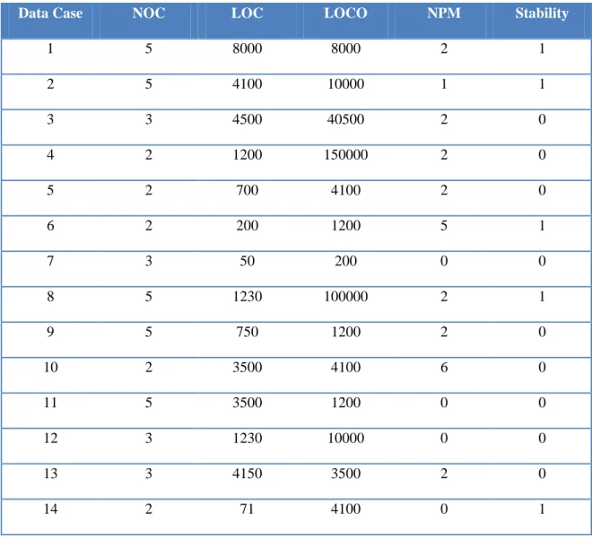
To illustrate as we proceed, we consider the case of predicting software stability. A data point is a vector of the form v = {a1,..., an, c} where ai is a metric and c is the classification label (0=stable, 1=unstable). A data point describes a class in an Object-Oriented system. A data set is formed of several such vectors. Table 3 shows an example of such a data set consisting of fourteen data cases, four metrics (NOC: Number Of

(26)

6

Children, LOC: Lines Of Code, LOCO: Lines Of Comments and NPM: Number of Public Methods), and one classification label (stable or not).

Table 3. Data set describing stability of classes in an Object-Oriented system

Data Case NOC LOC LOCO NPM Stability

1 5 8000 8000 2 1 2 5 4100 10000 1 1 3 3 4500 40500 2 0 4 2 1200 150000 2 0 5 2 700 4100 2 0 6 2 200 1200 5 1 7 3 50 200 0 0 8 5 1230 100000 2 1 9 5 750 1200 2 0 10 2 3500 4100 6 0 11 5 3500 1200 0 0 12 3 1230 10000 0 0 13 3 4150 3500 2 0 14 2 71 4100 0 1

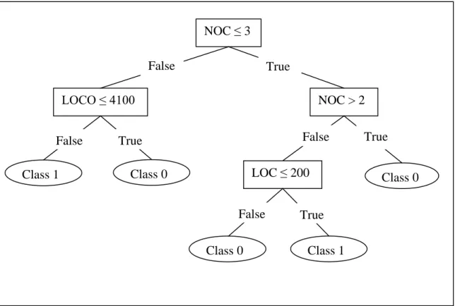
Prediction models establish a relationship between the unknown classification label and the metrics. One form of such models that has been widely used is decision trees. A sample decision tree constructed from the data set in Table 3 is shown in Figure

(27)

7

1. The decision tree is traversed starting from the root node down to a leaf. Once a leaf is reached, the classification label can be determined. Along the path, nodes encode tests and one whole path is a conjunction of such tests. For example, the left-most path in the tree inFigure 1reads as follows: “If NOC is more than 3 and LOCO is more than 4100, then the class is unstable.”

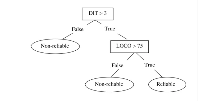
Decision trees can grow and become complicated to read by human experts. They can be transformed to rule sets. Figure 2 shows the extracted rule set from the decision tree in Figure 1. In this case, the rule set is composed of two rules and a default classification label. The default classification label is used to classify any case that does

NOC ≤ 3 LOCO ≤ 4100 Class 0 Class 0 Class 1 False NOC > 2 LOC ≤ 200 Class 1 Class 0 False True True False False

True False True

(28)

8

not match any of the rules. This is required because rule sets are formed after a pruning process which consists of eliminating tests from the decision tree as long as the

elimination does not deteriorate the accuracy of the tree.

The rule set is read as follows: if the class has a number of children (NOC) strictly greater than 3 and lines of comments (LOCO) strictly greater than 4,100 then it is unstable (classification label is 1). If the class has NOC less than or equal to 2 and lines of code (LOC) less than or equal to 200 then it is non-stable (classification label is 1). If neither Rule 1 nor Rule 2 applies to a particular class, then the class is stable (default classification label 0).

Such rule set models are widely used because they provide guidelines for

building a class with a particular software quality attribute. Normally, the quality of such rule sets is assessed using accuracy, error rate, the balanced accuracy, Sensitivity,

Specificity, and Precision. To illustrate these measures, we make use of the confusion matrix shown in Table 4. The confusion matrix is a 2x2 table, where 2 is the number of the classification labels (0 = stable and 1 = unstable).

Rule 1: NOC > 3 & LOCO > 4100  1 Rule 2: NOC ≤ 2 & LOC ≤ 200  1 Default class: 0

(29)

9

Table 4. Confusion matrix for binary classification Predicted label Positive Negative Real l abel Negati ve Posit

ive True Positive False Negative

False Positive True Negative

At each entry c[i] [j], we record the number of classes that were classified by the model with label j while their actual classification is i. To illustrate, we define a positive class label as a stable class (classification label 0) and a negative class label as a non-stable class (classification label 1).

True Positive (also known as hit): number of classes that are positive and were classified as such.

False Negative (also known as Type-II error or miss): number of classes that are positive but were classified as negative.

False Positive (also known as Type-I error or false alarm): number of classes that are negative but were classified as positive.

True Negative (also known as correct rejection): number of classes that are negative and were classified as such.

(30)

10

Assessing the rule set shown in Figure 2 on the data in Table 3, we obtain the confusion matrix shown in Table 5. Rule 1 applies to data cases 1, 2 and 8. Rule 2 applies to data cases 6 and 14. The default rule applies to data cases 3, 4, 5, 7, 9, 10, 11, 12 and 13.

Table 5. Confusion matrix by assessing rule set of Figure 2 Predicted label Positive Negative Real l abel Negati ve P osit ive 9 0 0 5

Let M be an estimation model. Eq.1 shows the accuracy of M. This equation computes the percentage of data cases which are correctly classified by M.

Eq.1

Eq.2 shows the error rate of M, also known as the overall misclassification rate.

(31)

11

Eq.2

In the case of an imbalanced data set with one classification label spanning most of it, accuracy stops being meaningful. Eq.3 shows the balanced accuracy. To illustrate, consider the case of a data set comprising 100 data cases. Ninety nine data cases have a classification label 0, and 1 data case has a classification label of 1. In such a case, a model assigning label 0 to all the cases has an extremely high accuracy (close to 100%). The problem ascends when the misclassification of the less frequent classification label is more costly, i.e. when class label 1 in the previous example refers to a diseased

individual but the model is classifying this case as a healthy individual who will not start his/her needed treatment. In this case, accuracy is not the appropriate measure to

consider. Instead, the balanced accuracy computes the average accuracy of the classification model hence giving equal weight to both classification labels.

Eq.3

Looking at Eq.3, it is important to note that the first portion of the balanced accuracy refers to the Sensitivity, whereas the second portion refers to the

(32)

12

Positive Rate (TPR) or recall or hit rate or probability of detection (PD) or completeness. Specificity is also known as True Negative Rate (TNR).

Eq.4

Eq.5

Another assessment measure is the Precision also known as Positive Predictive Value (PPV) or correctness, which is in general helpful to indicate the probability of the true positive cases out of all the positive cases. Precision is presented in Eq.6. In the case of reliability prediction, researchers are typically interested in this measure.

Eq.6

To illustrate, we use the confusion matrix of Table 6. Table 7 demonstrates the measurements computed from the confusion matrix of Table 6.

(33)

13

Table 6. Confusion matrix example Predicted label Positive Negative Real l abel Negati ve Posit ive 16 38 42 204

Table 7. Measurements computed from Table 6

Measurement Function Value

Accuracy (16 + 204) / 300 ≈ 0.73 Error Rate 1 - 0.73 ≈ 0.27 Balanced Accuracy 0.5* (16 / (16 + 38)) + 0.5*(204 / (204 + 42)) ≈ 0.565 Sensitivity 16 / (16 + 38) ≈ 0.3 Specificity 204 / (204 + 42) ≈ 0.83 Precision 16 / (16 + 42) ≈ 0.3

(34)

14

1.3 Problem Statement and Thesis Objective

Our goal is to optimize software quality prediction models. This is a computationally expensive task. Exact algorithms are almost impossible to build. This is why researchers in the domain have used heuristic-based approaches like Burgess and Lefley (2001), Azar, Precup, Bouktif, Kegl, and Sahraoui (2002), Bouktif, Sahraoui, and Antoniol (2006), Vandecruys, et al. (2008), Azar and Vybihal (2011), etc.

In this thesis, we areinspired from previous work and present a new Artificial Bee Colony algorithm for this purpose. To validate our approach, we benchmark it against known algorithms such as C4.51, as well as the three hybrid heuristics proposed by Azar, Harmanani, and Korkmaz (2009). The first hybrid combines Simulated

Annealing with Genetic Algorithms. The second hybrid combines Tabu Search with Genetic Algorithms. The third hybrid combines Simulated Annealing, Tabu Search and Genetic Algorithms. We also benchmark our ABC against a fifth approach which is the Genetic Algorithm proposed in (Azar & Precup, 2007). We also compare to two

versions of Multi-layer perceptron (MLP) (Farshidpour & Keynia, 2012): MLP with Back Propagation (MLP-BP) and MLP hybridized with ABC (MLP-ABC).

1

At the time of writing this thesis, C5.0 which is the successor of C4.5 was not publicly available for processing large data sets. Moreover, recent work still relies on C4.5 as the state-of-the art machine learning algorithm since C4.5 is found to perform better than C5.0 in classification problems (Visalatchi, Gnanasoundhari, & Balamurugan, 2014).

(35)

15

1.4 Thesis Organization

The remainder of the thesis is organized as follows: In Chapter 2, we thoroughly discuss the related work on Software Quality Estimation Models. In Chapter 3, we give a

background overview on the machine learning algorithm C4.5, since in our work we rely on C4.5 as input to our models. In Chapter 4, we present the proposed ABC model. In Chapter 5, we show how we conducted experiments and the results we obtained. In Chapter 6, we analyze the results. Finally, in Chapter 7, we conclude the thesis with final remarks and we state some open problems.

(36)

16

Chapter Two

Related Work

2 Related Work in Software Quality Estimation

In this chapter, we give an overview of existing work on Software Quality Estimation Models. In Section 1, we cover statistical models used in the estimation of software quality. In Section 2, we cover machine learning models. Finally, in Section 3, we cover the heuristic-based approaches used to build such estimation models.

2.1 Statistical Models

Statistical models have been widely used in the domain of software quality estimation. Mainly, they are models built using regression techniques, discriminant analysis, principle component analysis, etc.

Munson and Khoshgoftaar (1992) propose a discriminant analysis technique for detecting fault-prone programs. The objective is to reduce the initial set of metrics into a subset of non-correlated metrics. Two data sets related to a large commercial system from Lind and Vairavan (1989) form the experimental data. Results show that the approach classifies the programs with a low error rate.

(37)

17

Multiple linear regression analysis is proposed by Khoshgoftaar, Munson, Bhattacharya, and Richardson (1992) in which the authors use complexity metrics as indicators of change-prone software. Two subsystems of a general-purpose operating system from Kitchenham and Pickard (1987) and a medical imaging system (MIS) from Lind and Vairavan (1989) are used as experimental data. Khoshgoftaar, Munson,

Bhattacharya, and Richardson (1992) propose Relative Least Square (RLS) and

Minimum Relative Error (MRE). They compare their models to Least Square (LS) and Least Absolute Value (LAV). MRE shows to be superior to other techniques only when data is approximately normally distributed. In other cases, any other technique performs better than the proposed ones.

Khoshgoftaar, Munson, and Ravichandran (1992) examine the relationship of software complexity metrics and program modules that are most likely to be defect-prone. They propose a multidimensional scaling approach and test it on the data from Harrison and Cook (1987). They are able to distinguish between programs with and without errors. Hence, they emphasize the need of such statistical models to clearly understand the data at hand and to comprehend the underlying classification of the model.

A novel and enhanced regression model is proposed by Khoshgoftaar, Munson, and Lanning (1993). The methodology is based on initially applying principal

component analysis and then dividing the data into clusters. Each of those clusters would then be processed by the regression model. The approach is tested on the medical imaging system (MIS) from Lind and Vairavan (1989). The authors note a significant improvement in predicting software changes during maintenance.

(38)

18

Li and Henry (1993) investigate five Object-Oriented software metrics suite proposed by Chidamber and Kemerer (1994)2. They also propose five additional Object-Oriented metrics. Their approach is to build two least-square regression models whose dependent variable is the maintenance effort defined as the number of lines changed in a class. They experiment with several variations of the model by considering a different subset of the independent variables each time. Data is collected from two commercial software systems written in an Object-Oriented programming language (Classic-Ada). These two software systems are User Interface System (UIMS) and Quality Evaluation System (QUES). Empirical results prove the effectiveness of the used metrics in predicting maintenance effort and emphasize the importance of SIZE1 and SIZE2 as estimation metrics, where SIZE1 is the total number of semicolons in a class and SIZE2 is the total number of attributes and local methods in a class.

A hybrid approach is proposed by Khoshgoftaar and Szabo (1994) for improving the software estimation of gross change. The authors define gross change as “the number of lines added to, deleted from, or modified in a source module”. Initially, principal component analysis is applied to certain metrics chosen by the authors. This results in a set of metrics which form the independent variables of the regression model using stepwise regression and backward elimination. The dependent variable is the quality to be predicted. The authors then apply a multilayer perceptron neural network on the training data. The approach is tested on a system providing an interface between an operating kernel and its hardware. The authors conclude that neural networks provide

2

(39)

19

better predictive qualities than regression models, even though they require more time to train.

Briand, Morasca, and Basili (1994) show interest in the relationship between metrics and error-proneness. In order to validate the importance of the metrics, they fist use a univariate logistic regression model to evaluate the impact of each metric

independently. A multivariate logistic regression model is then performed to understand the impact of a combined set of the metrics. The three experimental data sets, which are written in Ada programming language, are the following: attitude ground support software for satellites supported by Goddard Space Flight Center (GOADA), a dynamic simulator for a geostationary environmental satellite (GOESIM) and an onboard

navigation system for satellite (TONS). The metrics Transitive Import Coupling (TIC) and Direct Import Coupling (DIC) are shown to be insignificant when used

independently in the case of TONS. TIC has a strong correlation with DIC in TONS and ISP has a strong correlation with DIC in GOESIM, so both TIC and ISP can be replaced by using DIC.

A well-known work is that of Fernardo and Walcelio (1996) who propose MOOD, a suite of metrics for Object-Oriented (OO) design. Their goal is to check the influence of OO design on software quality characteristics mainly maintainabilityand reliability. The authors come up with regression models to check the following outcome variables: Defect Density (DD), Failure Density (FD) and Normalized Rework Effort (NR). NR is a maintainability measure, whereas DD and FD are reliability measures. Experimental tests are done on eight small-sized information management systems, all having identical requirements. Results reveal how OO design metrics (such as

(40)

20

polymorphism, coupling, etc.) can indeed influence software quality characteristics (specifically maintainability and reliability).

Basili, Briand, and Walcélio (1996) conduct a similar work to Li and Henry (1993). They investigate the design metrics introduced by Chidamber and Kemerer (1994) and assess them as fault-proneness predictors. For this purpose, they propose univariate and multivariate logistic regression as a software quality estimation model. The collected data is related to the development of eight medium-sized information management systems written in a procedural programming language. All the systems are based on identical requirement. Experimental results assure the importance of such design metrics in fault-proneness estimation, since mostly all metrics (except LCOM) are correlated with defects.

An empirical comparison between several models is made by Lanubile and Giuseppe (1997) for fault-proneness estimation. They test the models on 27 software systems written in Pascal programming language. Eleven metrics are considered from the following category: size, control flow structure, data structure, coupling and one documentation metric. They implement the following models: discriminant analysis, principal component combined with discriminant analysis, logistic regression, principal component combined with logistic regression, logical classification models (C4.5 and ID3), layered neural network and holographic network. The best quality of the results is related to principle component analysis, followed by either discriminant analysis or logistic regression. Furthermore, it is shown that principal component is not necessarily related to better classifications. Therefore, the authors conclude that none of the models is able to accurately discriminate between fault and non-fault-prone components.

(41)

21

Another interesting work is that of Khoshgoftaar T. M., Allen, Halstead, Trio, and Flass (1998). The authors make use of the model history data as software metric to predict a module's reliability, specifically in JStars (Joint Surveillance Target Attack Radar System) a real-time military system developed by Northrop Grumman for the US Air Force in support of the US Army (Khoshgoftaar T. M., Allen, Halstead, & Trio, 1996). The authors' aim is to know whether a certain module is fault-prone or not, prior to integrating that module in the system. For that purpose, they apply logistic regression for building the classification model. They start by data splitting: 2/3 of the data is used for fitting the model and the remaining 1/3 is used for testing the model. Then, they set the dependent variable as the classification of the module as fault-prone or not, and the independent variables represent each module history. Then, they compute the accuracy of the resulting model classification to further improve the model. The results certify their hypothesis: modules that have a history of faults will most likely tend to have faults in the future. Also, when a sudden change occurs in either the code or a requirement, then faults are destined to occur. Their model would be very helpful to improve reliability of other systems as well, since it has low misclassification rates on testing data.

Khoshgoftaar and Allen (1999) propose a logistic regression-based classifier for fault-proneness estimation similar to the one in Khoshgoftaar T. M., Allen, Halstead, Trio, and Flass (1998). The originality of this work lies in applying prior probabilities as well as misclassification costs. They test their model on JStars. Empirical evidence proves that by correctly choosing the parameters of the model, the accuracy of the model will certainly be improved.

(42)

22

El Emam, Melo, and Machado (2001) build logistic regression models for fault estimation using data collected from Version 0.5 of a commercial word-processor Java application. They then validate the model Version 0.6 of the same application and the leave-one-out approach. The model uses a subset of Object-Oriented metrics related to inheritance, coupling metrics as well as two measures of size from Chidamber and Kemerer (1994) and Briand, Devanbu, and Melo (1997). Experiments show a high accuracy (more than 77%) and high J-Index (approximately 0.5) of their model. Moreover, the export coupling metric is found to have the strongest correlation with fault-proneness.

Subramanyam and Krishnan (2003) empirically test the effectiveness in fault-proneness estimation given a subset of the metrics proposed by Chidamber and Kemerer (1994). They build and train regression models on industry data from software

developed in C++ and Java programming languages. Interestingly, results show that the metrics are helpful predictors of fault-proneness, but their effectiveness varies across data from the two programming languages.

Schröter, Zimmermann, and Zeller (2006) show that import relationships, for example, knowing whether a class or package is imported from one version to another, can be good predictors of post-release failures. They build four models: linear

regression, ridge regression (which is a more generalized form of linear regression), regression trees and support vector machines. To compare them, they use precision, recall and Spearman’s coefficient. Empirical data consists of 52 ECLIPSE plug-ins. Linear regression shows good results on training data set, but the results deteriorate on testing data sets. Ridge regression has high precision values for estimation at the account

(43)

23

of a decreased recall. Regression trees and support vector machine out-beat both regression techniques, with the latter being the best out of all four approaches. Additionally, all approaches out-beat random guessing.

Zimmermann, Rahul, and Zeller (2007) address the question of “where do bugs come from?” For this reason, they collect data from Eclipse bug reports over three releases (2.0, 2.1 and 3.0). They train their logistic regression models to predict whether files/packages have post-release defects. They measure precision, recall and accuracy of the models. In the case of file defect-proneness estimation, it is noted that recall values are low meaning defect-prone files are rarely classified as defect-prone. The precision values are mostly above 0.5, indicating that there are few false positives. A key advantage is that the models learn from previous releases and gets high accuracy in classifying files in later releases. In the case of package defect-proneness estimation, results are higher suggesting that it is easier for the model to predict package defect-proneness than file defect-defect-proneness. A similar model is built for predicting which files/packages have most post-release defects. Similarly, the model is able to learn from previous releases.

Gao and Khoshgoftaar (2007) shed light on using Poisson regression model and the negative binomial regression model as effective software fault predictive models. The approaches are tested against a wireless telecommunication system. Results verify that both count models form good estimation models.

H. Zhang (2009) proves that the simple lines of code (LOC) metric is a useful predictor of pre-release and post-release defects. The author uses Eclipse and NASA

(44)

24

data sets3. Through hypothesis testing, the author confirms that larger modules tend to have more defects. The author also applies 10-fold cross validation with five

classification techniques: multilayer perceptron, logistic regression, naïve bayes, decision trees and K-Star. Concerning the Eclipse data, the techniques obtain good results for pre-release defect estimation: recall above 85%, precision above 71%, F-measure about 79% and accuracy about 70%. Also, for post-release defect estimation, the results are as follows: recall between 66% and 77%, precision between 63% and 68%, F-measure and accuracy both close to 70%. Similarly, the techniques show close results for the NASA data sets. Hence, this proves LOC as a valid predictor of defects.

Wang, Khoshgoftaar, and Napolitano (2014) present an original work in which they make use of wrapper-based feature subset selection; a classifier is used to discover the most useful feature subsets in fault-proneness estimation. Wrappers are “algorithms that use feedback from a learner or classifier to determine which subset of features to include for building a classification model”. They experiment with five variants of the approach depending on the choice of performance: Overall Accuracy (OA), Area Under ROC Curve (AUC), Area Under the Precision-Recall Curve (PRC), Best Geometric Mean (BGM) and Best Arithmetic Mean (BAM). Logistic regression is the underlying training method. They test on real-world Eclipse project from Zimmermann, Rahul, and Zeller (2007). The approach is deemed successful and BAM proved to be the best performance metric. As a conclusion, choosing a subset of metrics using a wrapper subset selector will improve the performance of defect estimation models.

3

The data sets used can be found in (Sayyad Shirabad & Menzies, 2005). They are the following: CM1, PC1, PC2, PC3, PC4, KC1, KC3, MC1 and MC2.

(45)

25

2.2 Machine Learning Models

One of the first work in machine learning models used for assessing software quality is by Selby and Porter (1988) where the authors use decision trees to classify a class in an OOP software system as fault-prone or not. They use sixteen software systems from NASA, each having up to one hundred thousand lines of code. They build around 9600 decision trees. An important result is that the produced decision trees vary largely in terms of complexity, accuracy and composition. Still, the decision trees have an average of 79.3% accuracy. Therefore, the authors show the validity of using decision trees for software quality estimation models.

Selby and Porter (1989) propose a recursive algorithm which automatically generates decision trees based on ID3 algorithm (Quinlan, 1986). The aim is to predict fault-prone as well as costly components. Experimental study is conducted on 16 NASA projects with 3,000 to 112,000 lines of code and on Hughes project data having more than 100,000 lines of code. The trees have an average accuracy of 79.3%. This work shows that classification trees are environment independent.

Porter and Selby (1990) consider classification trees to be effective in identifying fault-proneness based on software product metrics and software process metrics. The approach is validated on NASA used in Selby and Porter (1988) and Hughes project data used in Selby and Porter (1989).

Briand, Thomas, and Hetmanski (1993) emphasize the importance of decision trees as estimation models that are both useful and easily interpretable. They compare their Optimized Set Reduction model (OSR) (Briand, Basili, & Thomas, 1992) to that of

(46)

26

Logistic Regression described in Agresti (1990). The results prove how valuable OSR models are in software cost estimation.

Briand, Basili, and Hetmanski (1993) compare OSR to logistic regression (with and without principal component analysis), as well as to classification trees. An Ada system developed by NASA Goddard Space Flight Center is the basis of the

experiments, where the models identify a component as high or low risk. Results indicate that OSR gets the best result with a high rate of correctness (92.11%) and completeness (95.89%).

Khoshgoftaar, Lanning, and Pandya (1994) propose a neural network

classification model for classifying a program as fault-prone or non-fault-prone. The network takes as input 8 metrics, outputs a value between 0 and 1 (1 = fault-prone, 0 = non-fault-prone) and trains using backward propagation method. They test their approach against linear discriminant model using the Command and Control Communications System (CCCS), a large military telecommunications system implemented in Ada programming language. Results show that neural networks are capable of producing more accurate models.

Troster and Tian (1995) propose the use of tree-based models in order to uncover the relationships between defects (both pre and post-release defects) and software

metrics related to design, size, change, vocabulary and complexity from Card and Agresti (1988), Halstead (1977) and McCabe (1976). They use a large-scale legacy software system. The vocabulary and data complexity measures have stronger

correlation to defect estimation than structural complexity metrics. Results show how well-suited tree-based models are for guiding actions for quality improvement.

(47)

27

Khoshgoftaar T. M., Allen, Bullard, Halstead, and Trio (1996) apply a tree-based modeling method on JStars, a large tactical military system which is supposed to be highly reliable. The decision tree is developed from a single iteration of the life cycle of the system and the purpose is to predict the fault-proneness of each module in the next iteration. It is based on the TREEDISC algorithm (SAS, 1995) which is a refinement of CHAID algorithm (Kass, 1980). This paper is the first to apply this algorithm to metric-based data. Results show a 22.6% misclassification rate.

Gokhale and Lyu (1997) compare regression tree models to fault density technique in the case of predicting the number of faults in a software module related to medical imaging system (MIS) from Lind and Vairavan (1989). The tree is enlarged based on a certain value; the objective is obtaining a tree with the least deviance. To avoid over fitting, the tree is later pruned and 10-fold cross validation is applied. Eleven metrics are used: (Halstead, 1977), (Jensen & Vairavan, 1985), (McCabe, 1976), and (Jensen & Vairavan, 1985). The authors conclude that a regression tree is an effective way for data analysis, identification of troublesome modules and comprehension the relationship among data attributes. A key advantage is having a lower misclassification rate and deviance. They also indicate that optimizing a tree’s performance is an NP-complete problem.

Takahashi, Muraoka, and Nakamura (1997) experiment with a medium-sized network management software of 85,000 lines written in C programming language. They propose an improved classification tree of Porter and Selby (1990) generated using a new metric which is Akaike Information Criterion (AIC) (Akaike, 1987). The aim is to distinguish between high and low-quality modules using 45 used metrics comprising: (Halstead, 1977), (McCabe, 1976), (Henry & Kafura, 1981) and (Howatt & Baker,

(48)

28

1989). Their approach incorporates AIC in the construction of the tree and uses a small subset of complexity metrics without loss in the correct classification ratio (above 70%). This method is theoretically and experimentally proved to be more stable than that of Porter and Selby (1990). An important conclusion indicates that the re-use ratio is an important indicator of whether the resulting software is high or low-quality. Other important metrics for classification include Halstead’s mental effort (Halstead, 1977), Henry and Kaufra’s fan-out (Henry & Kafura, 1981) and Halstead’s distinct number of operands (Halstead, 1977).

Mao, Sahraoui, and Lounis (1998) investigate software reusability. They apply C4.5 with the windowing technique. They conclude that highly reusable components most likely have a low error complexity and a low volume measure than those of less reusable components.

Khoshgoftaar T. M., Allen, Naik, Jones, and Hudepohl (1999) present Classification And Regression Trees (CART) for building classification trees for software quality estimation models. The authors are inspired by the paper of Porter and Selby (1990). V-fold cross-validation is performed. They use 10-fold cross-validation, which is found to be sufficient according to Breiman, Friedman, Stones, and Olshen (1984). Experiments are based on applying CART on a large telecommunication system - consisting of ten million lines of code. The model's purpose is to predict whether or not modules have faults found by the customers.

Another well-known work on machine learning models is that of De Almeida and Matwin (1999) where the authors apply both machine learning and concept induction on a COBOL program to predict maintainability. The COBOL program is a

(49)

29

billing system belonging to the phone company Bell, Canada. The authors discuss how case selection, attribute selection, labeling, data analysis, model generation by the

learning program, model evaluation and model application are each an equally important part of the solution. Their model learns from the history of an organization. The model then provides an immediate interpretability of the results from certain induction techniques. Experimental tests use 19 metrics ranging from: (Halstead, 1977) and (McCabe, 1976). They compare their results to five other models from De Almeida, Lounis, and Melo (1998): NewID, CN2, C4.5, C4.5 rules and FOIL. It is found that all five are almost equal, FOIL having the lowest results. The evaluation of the model is based on its accuracy and completeness (i.e. comprehensibility) by the software organization. In the author's opinion, models based on C4.5 rules are the most comprehensible out of all five.

Khoshgoftaar T. M., Allen, Yuan, Jones, and Hudepohl (1999) apply a tree-based methodology to predict software fault-proneness. The generated model is correlated to the TREEDISC algorithm (SAS, 1995). A module is labeled as fault-prone if any faults were discovered by the customer. The basis for predictors is either the set of software product and execution metrics only or the set of software product, execution and process metrics. The system to train on is considered during two consecutive phases of its developments: after coding and after beta testing. Both models show satisfactory robustness, accuracy and parsimony. Therefore, classification trees are proven to be a helpful tool for analyzing full scale industrial software systems.

CART is also addressed by Khoshgoftaar T. M., Allen, Jones, and Hudepohl (1999), where the authors pose the question of “How long will a model yield useful

(50)

30

predictors?” They build two classification models and train them on 4 consecutive releases of a large telecommunication system written in Protel programming language. The first model is trained on the measurements of the first release and is validated over the three subsequent releases, whereas the second model is trained on the measurements of the second release and is validated over the subsequent two releases. The model’s aim is to predict fault-proneness. Its validity is measured as a ratio between the two types of misclassification. In total, forty-two metrics are used which are related to software product, process and execution. CART is shown to achieve balance between the two types of misclassifications. In addition, both models achieve a high accuracy

(approximately 70%), thus assuring the approach’s usefulness across all the studied releases.

Khoshgoftaar T. M., Allen, Yuan, Jones, and Hudepohl (1999) conduct an experimental study similar to that of Khoshgoftaar T. M., Allen, Bullard, Halstead, and Trio (1996). They use a tree-based model based on the TREEDISC4 (SAS, 1995). Over fifty metrics from call graphs, control low graphs, statement, software process and software execution metrics are put to use. However, in this study, the authors test the approach on a new data set related to a large telecommunication system written in Protel programming language in order to predict fault-proneness. In addition to that, in this study, they include 3 classification labels: fault-prone, not fault-prone and uncertain. Only 10.6% of the modules are uncertain and TREEDISC (SAS, 1995) is a well-suited algorithm in its nature to handle uncertain classifications. The model is also shown to be effective with a total misclassification rate of 26.9%. They conclude that their approach

4

(51)

31

is independent of the data itself, since in this study the approach is tested on a

telecommunication system, whereas in the previous study by Khoshgoftaar T. M., Allen, Bullard, Halstead, and Trio (1996), the same approach is tested on a military tactical system (JStars). Hence, the approach is tested on data from different domains.

Khoshgoftaar, Shan, and Allen (2000) apply regression trees from the S-Plus package on four large telecommunication systems. This paper reveals that the process and execution metrics were both especially important predictors of fault-proneness.

Yuan, Khoshgoftaar, Allen, and Ganesan (2000) address a fuzzy network approach. Fuzzy subtractive clustering predicts the number of faults which is then

passed to module-order modeling to ultimately predict whether the module is fault-prone or not. Data used is that of a large legacy telecommunication system. It is concluded that fuzzy networks can be effectively applied as a software quality estimation models.

Random forests, which are an extension of decision trees, are proposed by Guo, Ma, Cukic, and Singh (2004). The authors compare their methodology to logistic regression, discriminant analysis, WEKA, See5 and NASA’s ROCKY toolset. For this purpose, five NASA data sets related to mission critical software are selected: JM1, PC1, KC1, KC2 and CM1. 10-fold cross validation is applied. Random forests show the highest accuracy (75%-94%) and defect detection rate (up to 87%), especially on large-scale data sets.

Arisholm, Briand, and Fuglerud (2007) evaluate several techniques such as C4.5, PART, Support Vector Machines (SVM), logistic regression and neural networks for

(52)

32

fault-proneness models. They discover that C4.5performs well in terms of precision, recall and Receiver Operating Characteristic (ROC) area.

Lessmann, Baesens, Mues, and Pietsch (2008) use a large-scale empirical data comparison - 22 classifiers over 10 public data sets from NASA. The classifiers are: Linear Discriminant Analysis, Quadratic Discriminant Analysis, Logistic Regression, Naïve Bayes, Bayesian Networks, Least-Angle Regression, Relevance Vector Machine, k-Nearest Neighbor, K-Star, Multi-Layer Perceptron trained with a weight decay penalty to prevent over fitting, Multi-Layer Perceptron using Bayesian Learning paradigm, Radial Basis Function Network, Support Vector Machine (SVM), Lagrangian SVM, Least Squares SVM, Linear Programming, Voted Perceptron, C4.5 Decision Tree, Classification and Regression Tree, Alternating Decision Tree, Random Forest and Logistic Model Tree. The study results in the assurance that metric-based classification is in fact accurate and helpful. The authors add that there is no particular classification algorithm that is better than the other in terms of performance accuracy. They

recommend aspects of choosing the right classification method for a particular problem as ease of use, comprehensibility and computational efficiency.

Arisholm, Briand, and Johannessen (2010) compare the following classification techniques: logistic regression, neural network, C4.5 (and its variants), PART and Support Vector Machine (SVM). The authors show that the choice of the fault-prone modeling technique has limited impact on the accuracy or cost-effectiveness. Another important deduction states that what is considered as the best model is highly dependent on the criteria that is used to evaluate and compare the models.

(53)

33

Nugroho, Chaudron, and Arisholm (2010) make use of the history of a Java system in order to assess the UML-based estimation model. The cost-effectiveness of UML design metrics is emphasized for the fault-proneness estimation; mainly the “message detailedness” and “import coupling”. Message detailedness is computed by counting all sequence diagrams in which a particular object appears. Import coupling is related to the total number of incoming/outgoing method invocations to a particular object.

2.3 Heuristics and Metaheuristics

The main downfall for logical models is the fact that they do not predict as well on new, unseen data sets. For this purpose, heuristics and metaheuristics-based approaches have been proposed to improve the accuracy of such models on new/unseen data sets.

Previous work with such approaches, such as hybrids, Genetic Programming (GP), Genetic Algorithm (GA), Simulated Annealing (SA), Ant Colony Optimization (ACO), Particle Swarm Optimization (PSO) and Artificial Bee Colony (ABC) are discussed in this section.

2.3.1 Genetic Programming

The first work to propose Genetic Programming (GP) in software engineering in general is that of Khoshgoftaar, Evett, Allen, and Chien (1998) and Evett, Khoshgoftaar, Chien, and Allen (1998). GP approach is introduced specifically for reliability

(54)

34

metrics used are related to lines of code, operator and cyclomatic complexity (McCabe, 1976). The metrics are proved to be associated with reliability estimation according to Fenton and Pfleeger (1993) . In this study, the evaluation of the GP relies on Pareto’s law which implies that “20% of the modules will typically account for about 80% of the faults.” The approach is found to be robust as opposed to random model when tested on two large industrial projects: Ada-written Command Control and Communications System (CCCS) and Pascal-written legacy telecommunication system.

Another GP approach is proposed by Liu and Khoshgoftaar (2001) to predict fault-proneness and change-proneness using large Windows-based applications written in C++ programming language. Accounting for over-fitting, GP only uses a random subset selection of the data. GP is then tested on the entire data set given product and process metrics. The proposed GP is novel in the sense that it integrates prior probability as well as misclassification cost into its fitness function. It is demonstrated that, when compared to logistic regression, GP achieves better results in terms of I and Type-II errors. GP also obtains an average of 9% improved accuracy over logistic regression.

Software effort estimation using public domain metrics is addressed by Lefley and Shepperd (2003). They use the “Finnish data set” collected by the software project management consultancy organization called SSTF (Maxwell, Van Wassenhove, & Dutta, 1999). They compare GP to the following models: random, Least Square Regression, Nearest Neighbor, Artificial Neural Network and the average of all non-random estimators. Results are not conclusive as to which model performs better in general. However, on the particular data at hand, the GP did obtain good results.

(55)

35

Khoshgoftaar, Seliya, and Liu (2003) propose a fault-proneness estimation model which incorporates decision trees within the Strongly Typed GP (STGP) model5. They use four product metrics related to the number of lines and one process metric related to the “number of times the source file was inspected prior to system test.” The approach has a multi-objective fitness function: one related to the minimization of the average weighted cost of misclassification and another one controlling the size of the output decision tree. The approach is tested on an industrial high-assurance software system and compared to standard GP. In terms of Type-I and Type-II misclassification, STGP out-performs standard GP by at least 2.5%. Thus, the importance of this work lies in showing how well GP performs with the existence of multiple conflicting objective functions.

In order to tackle the problem of over fitting, Liu and Khoshgoftaar (2004) propose a GP approach. The GP’s fitness function is multi-objective similar to that of Khoshgoftaar, Seliya, and Liu (2003). Twenty-eight software metrics and four execution metrics are collected by Khoshgoftaar, Cukic, and Seliya (2002). The approach is tested on a large legacy telecommunication system written in Protel programming language. The GP is trained using the Random Sampling Technique (RST), and the

misclassifications of Type-I and Type-II are measured. Results show how effective it is to incorporate RST with GP in order to improve the misclassification rates by 1% to 8%.

Yongqiang and Huashan (2006) propose GP for predicting software reliability based on Mean Time Between Failures (MTBF). When compared to some statistical

5