Open PRAIRIE: Open Public Research Access Institutional
Open PRAIRIE: Open Public Research Access Institutional
Repository and Information Exchange
Repository and Information Exchange
Electronic Theses and Dissertations2019
Finite Mixture of Regression Models for Complex Survey Data
Finite Mixture of Regression Models for Complex Survey Data
Abdelbaset Abdalla
South Dakota State University
Follow this and additional works at: https://openprairie.sdstate.edu/etd
Part of the Statistics and Probability Commons
Recommended Citation Recommended Citation
Abdalla, Abdelbaset, "Finite Mixture of Regression Models for Complex Survey Data" (2019). Electronic Theses and Dissertations. 3629.
https://openprairie.sdstate.edu/etd/3629
This Thesis - Open Access is brought to you for free and open access by Open PRAIRIE: Open Public Research Access Institutional Repository and Information Exchange. It has been accepted for inclusion in Electronic Theses and Dissertations by an authorized administrator of Open PRAIRIE: Open Public Research Access Institutional Repository and Information Exchange. For more information, please contact [email protected].
BY
ABDELBASET ABDALLA
A dissertation submitted in partial fulfillment of the requirements for the Doctor of Philosophy
Major in Computational Science and & Statistics South Dakota State University
DISSERTATION ACCEPTANCE PAGE
This dissertation is approved as a creditable and independent investigation by a candidate for the Doctor of Philosophy degree and is acceptable for meeting the dissertation
requirements for this degree. Acceptance of this does not imply that the conclusions reached by the candidate are necessarily the conclusions of the major department.
Advisor Date
Department Head Date
Dean, Graduate School Date
Abdelbaset Abdalla
Semhar Michael
ACKNOWLEDGMENTS
This Dissertation would never have been possible without the help and support of my parents and my wife. I would firstly like to express my deepest gratitude to my supervisor, Professor Semhar Michael, for her continuous support from the initial to the final level, for her great patience, motivation, excellent guidance, and immense knowledge. I could not have imagined having a better or friendlier supervisor.
Most importantly, I would also like to thank my committee members Dr. Christopher Saunders, Dr. Gary Hatfield, and Dr. Zhiguang Wang. I have a great deal of respect for each of you, you all have very different careers, and I have learned so much by working with each one of you. I would like to thank the University of Benghazi for scholarship and their financial support.
I am very grateful for Dr. Kurt Cogswel and Mathematics & Statistics Department for their financial support for the first arrival and for giving me this opportunity.
Also, I would like to thank South Dakota State University and the Brookings commu-nity for accepting me to complete my study and for all of the lifetime memories that I got during my stay in the United States.
Finally, I would like to thank my parents, sisters, my wife, and my dear kids, for always supporting me and encouraging me with their love and best wishes.
CONTENTS
LIST OF FIGURES x
LIST OF TABLES xii
ABBREVIATIONS xiii
NOTATIONS xiv
ABSTRACT xv
1 INTRODUCTION 1
1.1 Literature Review of Sampling Designs . . . 4
1.2 Literature Review of Sampling Weights . . . 5
1.3 Review of Finite Mixture Regression Models . . . 7
1.4 Outline of the Dissertation . . . 8
2 METHODOLOGY 10 2.1 Complex Survey Design . . . 10
2.1.1 Stratified Sampling . . . 12
2.1.2 Cluster Sampling . . . 13
2.1.3 Complex Sampling . . . 14
2.2 Gaussian Mixture Models . . . 16
2.2.1 Pseudo-Maximum Likelihood Estimation of Gaussian Mixture Mod-els . . . 18
2.2.2 Multivariate Gaussian Finite Mixture Models . . . 19
2.3 Finite Mixture of Gaussian Regression Model . . . 20
2.3.2 Pseudo-Maximum Likelihood Estimation of Mixture Gaussian
Re-gression . . . 23
2.3.3 Matrix Approach for the Mixture of Gaussian Multiple Regression Models . . . 24 2.4 Computational Strategies . . . 24 2.5 Identifiability . . . 25 2.6 Model Comparison . . . 26 2.7 Variability Assessment . . . 27 3 SIMULATION STUDIES 30 3.1 Simulation of Stratified Sampling Data . . . 30
3.1.1 Simulation 1: Parameter Estimation of Stratified Sampling Data . . 30
3.1.2 Simulation 2: Model Comparison of Stratified Sampling Data . . . 35
3.1.3 Simulation 3: Model Selection of Stratified Sampling Data . . . 37
3.2 Simulation Studies of Cluster sampling Data . . . 41
3.2.1 Simulation 1: Parameter Estimation of Cluster Sampling Data . . . 41
3.2.2 Simulation 2: Model Comparison of Cluster Sampling Data . . . . 46
3.2.3 Simulation 3: Model Selection of Cluster Sampling Data . . . 47
3.3 Simulation Studies of Complex Sampling . . . 52
3.3.1 Simulation 1: Parameter Estimation of Complex Sampling Data . . 52
3.3.2 Simulation 2: Model Comparison of Complex Sampling Data . . . 57
3.3.3 Simulation 3: Model Selection of Complex Sampling Data . . . 60
4 APPLICATIONS 63 4.1 Application to Data from Stratified Sampling Design . . . 63
4.1.1 Example 1: Academic Performance Index . . . 63
4.1.2 Example 2: Academic Performance Index . . . 66
4.2.1 Example 1: Mixture of linear regression models for Systolic Blood
pressure . . . 68
4.2.2 Example 2: Mixture of Linear Regression Models for Total Choles-terol . . . 70
4.3 Application to Data from Complex Survey Design . . . 71
4.3.1 NHANES Dataset . . . 72
4.3.2 Approach . . . 73
5 CONCLUSIONS AND FURTHER RESEARCH 80 5.1 Summary . . . 80
5.2 Further Research . . . 83
A APPENDIX 84 A.1 Asymptotic Properties of the ML Estimators . . . 84
A.2 Properties of ML Estimator for Mixture Models . . . 86
A.3 The Pseudo-Likelihood Approach . . . 90
A.3.1 Conditions for Consistency . . . 91
A.3.2 Conditions for Asymptotic Normality . . . 92
B APPENDIX 95
BIBLIOGRAPHY 142
LIST OF FIGURES
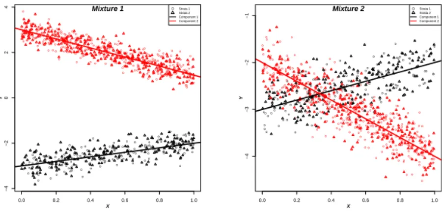
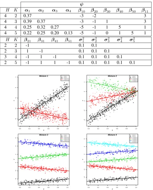
1.1 Diagrams representing classical design-based inference (on the left), model-based inference for super-population parameters (on the right). . . 3 3.1 Scatter plots of a sample of size n = 1000 units. Colors show the two
components and plotting characters represent strata. Left plot represents Mixture 1 - non-overlapping components and right plot represents Mixture 2 - overlapping components. . . 32 3.2 Summary of the R index for bias (top row), variance (middle row), and
mean squared error (bottom row) in Simulation study 2. The middle line represents the median and the dashed bars represent the interquartile range (IQR) values at different sample sizesn. . . 38
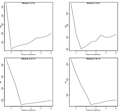
3.3 Scatter plots of samples which are selected from finite populations for the four experiments in Simulation 3. Colors show the number of components, and plotting characters show the strata. . . 40 3.4 BIC values corresponding to the optimal number of components for the
four experiments. . . 40 3.5 Scatter plots of a sample of size n = 1000 units. Colors show the two
components and plotting characters represent clusters. The left plot repre-sents Mixture 1 - non-overlapping components, and the right plot represent Mixture 2 - overlapping components when cluster sampling design was considered. . . 42 3.6 Summary of the R index for bias (top row), variance (middle row), and
mean squared error (bottom row) in Simulation study 2. The middle line represents the median and the dashed bars represent the interquartile range (IQR) values at different sample sizesn. . . 48
3.7 Scatter plots of samples selected from finite populations for the four ex-periments in Simulation 1. Colors show the number of components and plotting characters show the clusters. . . 50 3.8 BIC values corresponding to the optimal number of components for the
four experiments. . . 51 3.9 Scatter plots of a sample of size n = 1000 units. Colors show the
com-ponents, and plotting characters represent the eight strata as primary sam-pling units (PSU’s) from where the sampled units were drawn. The left plot represents Mixture 1 - non-overlapping components, and the right plot represent Mixture 2 - overlapping components. . . 54 3.10 Summary of the R index for bias (top row), variance (middle row), and
mean squared error (bottom row) in Simulation study 2. The middle line represents the median and the dashed bars represent the interquartile range (IQR) values at different sample sizesn. . . 59
3.11 Scatter plots of samples selected from finite populations for the four exper-iments in Simulation 3. Colors show the number of components, and plot-ting characters represent the eight strata as primary sampling units from where the sampled units were drawn. . . 61 3.12 BIC values corresponding to the optimal number of components for the
four experiments. . . 62 4.1 The plot shows the best-fitted mixture regression model with a 2-component
quadratic Gaussian regressions model to regress the academic performance index in 2000 for the students on percent parents who are high-school grad-uates . . . 65
4.2 Plots show (a) BIC versus to the number of components, for the mixture regression model of regress the API in 2000 for students on percent of parents with some college, (b) the fitted mixture regression model with a 2-component for the same dataset. . . 67 4.3 Plots show (a) BIC versus to the number of components, for the mixture
regression model of regress systolic blood pressure on the body mass in-dex level (on the left), (b) the fitted mixture regression model with a 2-component for the same dataset (on the right). . . 69 4.4 Plots show (a) BIC versus to the number of components, for the
mix-ture regression model of regress the total cholesterol on the direct HDL-cholesterol (on the left), (b) the best fitted mixture regression model with a 2-component of the same dataset (on the right). . . 71 4.5 The plot shows BIC versus the number of components, for a mixture of
multiple regression models of regress the systolic blood pressure on the body mass index, age, and blood lead levels. . . 74 4.6 plots show the best-fitted mixture of multiple regression models with a
3-component to regress the systolic blood pressure versus three auxiliary variables for NHANES data. . . 74 4.7 The plot shows the proportion of classification solutions agreement
LIST OF TABLES
3.1 True parameter values for Mixture 1 and Mixture 2. . . 31 3.2 Mean squared error, bias, and variance of estimated parameters, based on
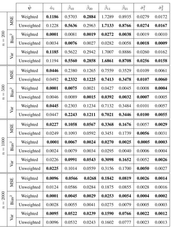
1000 replications for different sample sizes of the two-component when the Mixture 1 configuration was considered under stratified sampling design. The values reported are×10−2. . . 33
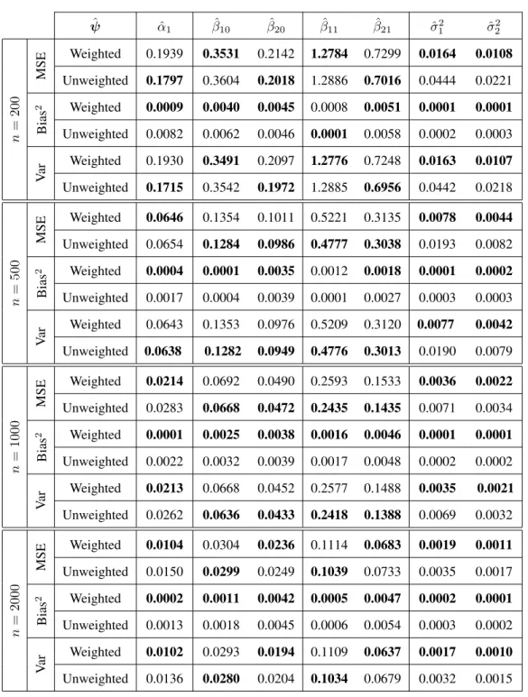
3.3 Mean squared error, bias, and variance of estimated parameters, based on 1000 replications for different sample sizes of the two-component when the Mixture 2 configuration was considered under stratified sampling design. The values reported are×10−2. . . 34
3.4 True parameter values for Mixtures of linear regression in Simulation 3. . . 39 3.5 True parameter values for Mixture 1 and Mixture 2 considering cluster
sampling design. . . 42 3.6 Mean squared error, bias, and variance of estimated parameters, based on
1000 replications for different sample sizes of the two-component when the Mixture 1 configuration was considered under cluster sampling design. The values reported are×10−2. . . . 44
3.7 Mean squared error, bias, and variance of estimated parameters, based on 1000 replications for different sample sizes of the two-component when the Mixture 2 configuration was considered under cluster sampling design. The values reported are×10−2. . . 45
3.8 The true parameters used for simulating Mixtures of linear regression in Simulation 3. . . 50 3.9 True parameter values for Mixture 1 and Mixture 2 considering complex
3.10 Mean squared error, bias, and variance of estimated parameters, based on 1000 replications for different sample sizes of the two-component when the Mixture 1 configuration was considered under complex survey design. The values reported are×10−2. . . . 55
3.11 Mean squared error, bias, and variance of estimated parameters, based on 1000 replications for different sample sizes of the two-component when the Mixture 2 configuration was considered under complex survey design. The values reported are×10−2. . . 56
3.12 True parameter values for Mixtures of linear regression in Simulation 3. . . 61 4.1 BIC values for combination of number of componentsKand degree of the
polynomialrin Example 1. Bold font represents the lowest BIC obtained
indicating the best fit. . . 65 4.2 Estimated parameters for the mixture regression model for the data in
Ex-ample 1. . . 65 4.3 Parameters estimated for the mixture regression model with the response
the academic performance index in 2000 for the students and the percent of percent parents with some college as explanatory variable. . . 66 4.4 Estimated parameters for the mixture regression model with the response
variable systolic blood pressure and the body mass index as explanatory variable. . . 69 4.5 Estimated parameters for the mixture regression model when regress the
ABBREVIATIONS
API . . . Academic Performance Index.
BIC . . . Bayesian information criterion.
CS . . . Complex sample.
EM . . . The expectation maximization algorithm.
FMR . . . Finite mixture of regression.
IID . . . Independent identically distributed.
IQR . . . Interquartile range.
MOM . . . Method of moments.
MLE . . . Maximum likelihood estimation.
MSE . . . Mean Squared error.
NCHS . . . National Center for Health Statistics.
NHANES . . . National Health and Nutrition Examination Survey.
PML . . . Pseudo maximum likelihood.
PSU . . . Primary sampling unit.
SRS . . . Simple random sample.
NOTATIONS
αk: The mixing proportion ofkth component.
βk: The regressions coefficients ofkth component. K: The total number of mixture regression components. Mi: Number of population units inith selected cluster mi: Number of elements in the sample from theith PSU. N: Population size
n: Sample size.
Nh: Number of sampling units (PSU’s) in stratumh, h= 1, ..., H. nh: Number of PSU’s sampled from stratumh, h= 1, ..., H. Nc: Number of (PSU’s) clusters in the population.
nc: Number of (PSU’s) clusters in the sample. π: Inclusion probability of a sampling unit.
Ψ: The parameter vector.
σ2
k: The variance ofkth component.
R: Percent contribution Index.
U: Finite population
Wk(t):n×ndiagonal matrix with entrieswi×τik(t).
X:n×(p+ 1)matrix containing unity for intercept and predictors.
ABSTRACT
FINITE MIXTURE OF REGRESSION MODELS FOR COMPLEX SURVEY DATA
ABDELBASET ABDALLA 2019
Over time, survey data has become an essential source of information for modern so-ciety. However, to be effective, the structures of survey data require sampling designs that are more complex than simple random sampling. The complex sampling data collected from enormous national surveys via these complex designs ideally include sample weights that allow analysis to take account of complicated population structures. When the target of inference is the parameters of a regression model, it is crucial to know whether these weights should be incorporated into the sampling weight when fitting the model to the sur-vey data. The finite mixture models are one tool for modeling heterogeneity and finding the subgroups in the data. Limited literature is available on modeling survey data via the finite mixture of regression models using a complex survey design.
The principal aim of this dissertation is to develop and evaluate strategies for survey data modeling using a new design-based inference, where sampling weights are integrated into the complete-data log-likelihood function. More specifically, the pseudo maximum likelihood estimator (PML) has been considered, so the expectation-maximization (EM) algorithm was developed accordingly. In order to evaluate this strategy in realistic circum-stances, we simulated the performance of the proposed model under numerous scenarios. Comparisons were made using bias-variance components of the mean squared error. Ad-ditionally, the Bayesian information criterion was utilized and assessed as a selection tool under the proposed modeling approach. Finally, we applied the proposed approach to orig-inal survey datasets to assess its practical usefulness
1 INTRODUCTION
In modern society, survey accumulated data provides significant statistics in ultimately creating a positive philosophy of change. Accurate facts gathered though surveys become instrumental in the process of making decisions. Vital decisions include the implementa-tion of program adjustments to better address the needs of a populaimplementa-tion, the improvement of community policies and projects, creating priorities when allocating funds in regard to government agencies, and public queries. Data and evidence combined from different surveys facilitates the progress of health issues globally. In this framework, evidence col-lected from social surveys, one of the most essential data sources, enables understanding of changes in societal social trends, empowering the examinations of change for the benefit of citizens as well as communicating a vision on issues specific to social policy. Equally, health survey data plays a fundamental role in advising policymakers, as well as the public, regarding significant health issues implemented by strategies and procedures. Therefore, survey data contributes the most vital evidence to a focused and successful decision-making processes concerning the implementation of government and global policies. Reliable and unbiased methods of attaining information from a survey commands scrutiny particularly since this information creates the basis for making choices affecting large target popula-tions. Specifically, the necessity to establish dependable survey methods must launch with a small sample in order to consider and infer characteristics of relationships of a vast popu-lation. Multifaceted survey datasets contain distinctive structures that require an analytical approach that cannot be achieved using standard techniques. Therefore, necessities for the development of statistical methodologies intensify in order to extract information from data collected from complex survey designs. Statistical sampling techniques and the analy-sis of complex survey data is detailed in Kish (1965), Cochran (1977), Kalton and Graham (1983), Lohr (2010), and in a more current issue published in the statistical science journal
(Zhang, 2017).
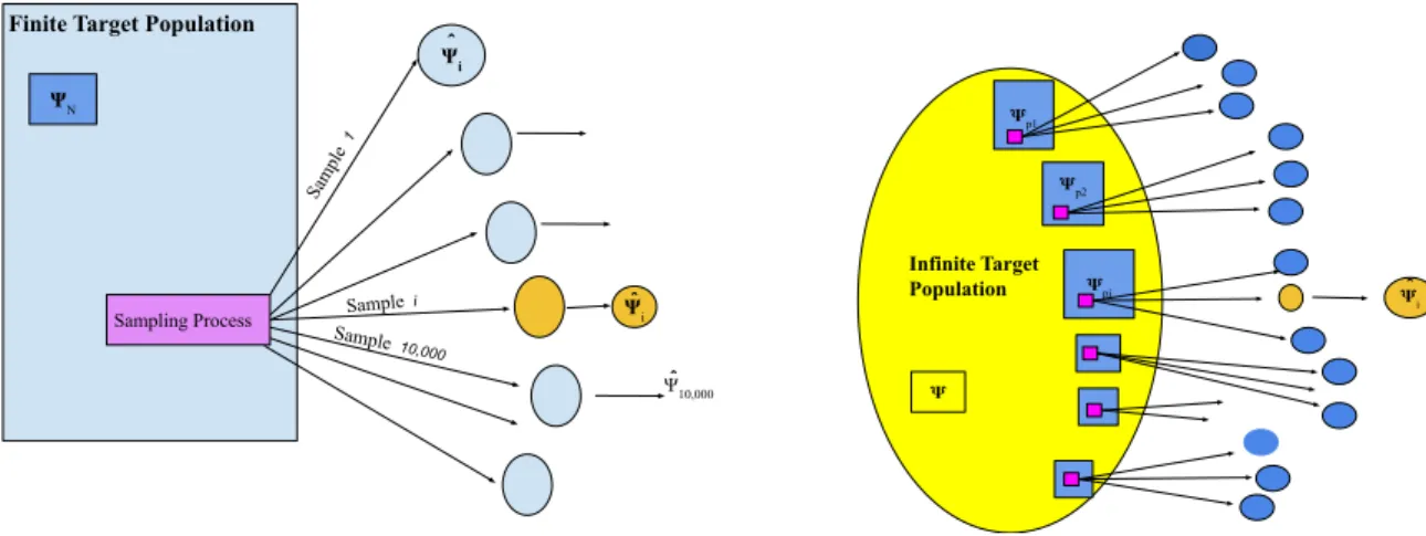
The bulk of all-encompassing surveys use two principal methodologies of statistical in-ference; namely, design based and model-based inference. These tactics incorporate com-plexities into survey sampling, such as clustering, stratification, and unequal probabilities of the selection mechanism. In the 1950s, model-based analysis began by Godambe (1955) and Royall (1968). Design-based analysis initiated by Neyman (1934) is used in the frame-work of survey sampling design to generate inference for population limitations. If we consider the superpopulation model and letΨN to be a finite population estimator for the
model parameterΨ, which could be computed if the entire populationU was observed. If
the components of the parameter vectorΨN can be expressed as functions of a finite
pop-ulation parameter, it is again possible to estimate it by a design-based estimator. However, the model-baIf we consider the superpopulation model and letΨN to be a finite population
estimator for the model parameter Ψ, which could be computed if the entire population
U was observed, if the components of the parameter vectorΨN can be expressed as
func-tions of a finite population parameter, it is again possible to estimate it by a design-based estimator. However, the model-based is viewing the target population itself as a random realization from the superpopulation model. In this view, the finite population quantityΨN
is viewed as one particular realization of an estimator of the superpopulation model param-eterΨ. Figure 1.1 illustrates the traditional view of the design-based and model-based. In
this dissertation, a design-based technique used as an analysis tool, for a given dataset gath-ered using complex sampling design, will be considgath-ered. Principally, the design considers the complication of finite mixture linear regression analysis in order to analyze complex survey data.
Sampling Process
ΨN
Ψ^i Finite Target Population
^ Sample i ^ Ψ10,000 Sample 1 Sample 10,000 Ψi ƁN Infinite Target Population 𝚿 𝚿p1 𝚿p2 𝚿pi 𝚿^ i
Figure 1.1: Diagrams representing classical design-based inference (on the left), model-based inference for super-population parameters (on the right).
Contemporary statistical applications widely use regression analysis. Essentially, re-gression analysis demonstrate a path of responses based on its relationship with one or more predictor or explanatory variables. Commonly, applications of linear regression evaluate independent identically distributed (IID) data. However, when investigators perform re-gression analysis on survey data the assumption is repeatedly inadequate in complex survey sampling designs. Subsequently, linear regression models and estimators typically apply to the inquiry of complex survey data using the PML method first recommended by Binder (1983) following the idea from Skinner et al. (1989). DuMouchel and Duncan (1983) have been discussed the sampling weights in multiple regression analysis for stratified samples. Survey designs through strata, cluster, or a combination of the two, strive to capture the heterogeneity in population in a more economical way. Nonetheless, occasionally subpop-ulations occur after data collection. One malleable technique for modeling heterogeneity in data uses finite mixture models (McLachlan and Peel, 2000). Finite mixture regression models (Leisch, 2004; Grün and Leisch, 2008) permit simultaneous outcomes of original subpopulations and structuring a regression model for each subpopulation in the data. Cor-respondingly, this dissertation explores fitting finite mixture linear regression models to sample survey data by including sampling weights to the regression parameter estimators.
1.1 Literature Review of Sampling Designs
Consider a finite population U, comprised of a set ofN units termed 1, ..., N, and a
vector of parameters of interest,Ψ, to be assessed. Supposing having used the entire
popu-lation to estimateΨ, but regrettably, the population usually exceeds the amount, increasing
cost, or too complex to pull together the required statistics from each population division to analyzeΨ. Hence, one obtains a sample of sizenfrom the population, which provides the
data with whichΨcan be estimated. Let this estimator be represented byΨb. The quality
of the precision of Ψb as an estimator of Ψ depends on, amid other factors, how closely
the sample exemplifies the population of interest. An impeccable sample would be similar to Grand view: a scaled-down version of the population, reflecting every distinctive fea-ture of the entire population. Indubitably, such an idyllic sample cannot occur for complex populations. As an alternative, effective sampling ensures that the characteristic of impor-tance in the population,Ψ, can be estimated from the sample byΨb and the precision of the
estimation can be calculated (Lohr, 2010).
Sampling methods split into two classifications, a probability or a non-probability sam-pling technique. The methodology behind non-probability techniques, such as convenience or purposive sampling, automatically eliminates specific population units from the sampled population due to techniques that choose sample units via subjective evaluation. In general, this form of sample selection causes the estimate,Ψb, to be biased. Moreover, in the absence
of any probability techniques in the selection process, the degree of bias is indefinite. Any effect concluded from non-probability samples subjects itself to an unidentified level of bias (Lohr, 2010). A vital necessity of a probability sampling techniques certify that each possible sample of size naccumulated from the finite population has an identified
proba-bility of being selected (Chen et al., 2017). The use of a random mechanism to establish population units selected for the sample reduces the possibility of altering a pre-selected unit for a different unit based on personal judgment. Henceforth, by means of the appli-cation of a probability sampling technique, each individual population unit has an assured
chance of appearing in the sample. The possibilities underlying all potential samples of size
ngathered using a probability sampling technique allow the establishment of the sampling
distribution ofΨb, the estimator ofΨ, making it possible to detect inference usingΨˆ and
likewise defining the quality of the inference by means of the evaluation of standard errors, biases, etc. of the estimators Lohr (2010). Common types of probability sampling include simple random sampling, cluster sampling, stratified sampling, and multistage sampling. Complex sampling, which contrasts with simple random sampling, applies one or more unequal random selection mechanisms. The most popular designs involve using stratified sampling and cluster sampling, or any combination of sampling designs. One might want to consider complex survey design as opposed to simple random sampling as the list of the population may not be available, and even if it is, it might be extremely inefficient to col-lect data. Besides, any analysis of complex survey data that ignores both sample weights and the sampling design may lead to biased estimation and inaccurate inference. For sta-tistical inference, when studying survey sample data, considering the sampling design is imperative. In chapter 2, reviews of properties of estimates for the principal design mech-anisms used in a probability and sample survey design contain stratified, cluster sampling, and complex sampling. The integration of these ideas in section 4.3 demonstrates how they work collaboratively in complex surveys such as the National Health and Nutrition Examination Survey (NHANES).
1.2 Literature Review of Sampling Weights
The primary objective of the sampling theory is to gain insights concerning population parameters of interest. So, insights about those population parameters of interest can be inferred from the sample. Therefore, the importance of employing sampling weights in inference is to adjust for imperfections, for instance, unequal probabilities and population groups that are not adequately embodied in the particular sample. The use of probability
sampling techniques enables the determination of the inclusion probability of a population unit in the acquired sample. Let the inclusion probability of the ith population unit be
defined asπi and letwi denotes the design weight. The most common definition of
sam-pling weight is as an indicator of the number of population units that are represented byith
sample unit.
The sampling weights in the first stage are assigned to each sample unit to adjust for the unequal selection probabilities. Thus, the sampling weights might not be inverse of inclusion probability. The sampling weights are modified for several reasons. Some cus-tomary corrections include nonresponse, misspecification of the sampling frame, and post-stratification. The weights extend the clear-cut idea of design weights by incorporating auxiliary population data. An assortment of adjustments can be executed, and the forma-tion of weights can be complex. Further details regarding weighing in complex surveys can be found in Kish (1992), Gelman et al. (2007), Särndal (2007), Haziza and Lesage (2016); Haziza et al. (2017), and Chen et al. (2017). In this dissertation, it is presumed that the sampling weights are inverse of the inclusion probability of a population unit being selected for the sample,
wi = 1
πi, i= 1, ..., n,
wheren is the size of the selected sample and is interpreted as the number of population
units represented by the ith sampled unit. Subsequently N = Piwi , the size of the
population from which the sample is selected (Horvitz and Thompson, 1952; Lohr, 2010). Whenever we are dealing with a real-life data application, we either compute the weights associated with each observation based on the sampling design or use the already existing weights available with the data.
1.3 Review of Finite Mixture Regression Models
In the nineteenth century, finite mixture models made their initial recorded appear-ance in modern statistical literature by Newcomb (1886) who used it in the framework of modeling outliers. In the years following, Pearson (1894) applied a mixture of two uni-variate Gaussian distributions to analyze a dataset containing ratios of the forehead to body lengths for 1,000 crabs, using the method of moments (MOM) to estimate the parameters in the model. The most prevalent mixture model is the one consisting of Gaussian compo-nents (Day, 1969; McLachlan and Basford, 1988; Fraley and Raftery, 2006). We refer to McLachlan and Peel (2000) and Frühwirth-Schnatter (2006) for a complete survey on the history and applications of finite mixture models.
Universally, finite mixture models are used to model data from a heterogeneous pop-ulation. The power of finite mixture models through model-based clustering is that they allow us to cluster and classify with the assumption that each mixture component rep-resents a set of an observation belonging to one group in the original data (McLachlan and Basford, 1988; Fraley and Raftery, 1998). Various fields of statistical applications such as medicine and biology use mixture distributions for many purposes see, for exam-ple„ the review chapter in Schlattmann (2009). All-encompassing dialogue concerning the derivations and applications of finite mixture models are presented in the monographs by McLachlan and Peel (2000) and Frühwirth-Schnatter (2006), and more recent reviews by Melnykov et al. (2015); McNicholas (2016); McLachlan et al. (2019) discusses recent advances and challenges in the topic of finite mixture models and model-based clustering
When a random variable with finite mixture distribution depends on some covariates, it acquires a finite mixture of regression (FMR) model (Khalili and Chen, 2007). The ba-sic idea here is to be able to fit different regression models to portions of data that behave similarly. Quandt and Ramsey (1978) introduced mixtures of linear regression models as a very basic method of switching regression. De Veaux (1989) established an EM approach to fit the two regression situations. Jones and McLachlan (1992) applied combinations of
regressions in data analysis and applied the EM algorithm to suit these models. Applica-tions of FMR models, in many capacities such as market segmentation and social sciences, are studied more carefully in Wedel and Kamakura (2012) and Rabe-Hesketh and Skrondal (2004). The model is implemented in theRsoftware through theFLEXMIXpackage (Grün
and Leisch, 2008).
Fitting regression models to survey data complicates estimating pure population quan-tities such as totals, means, quantiles and variances. In addition, one of the commonly sought after parameters is the census regression coefficient. This is what would be reached from a regression if the complete population had been sampled. In most detailed demon-stration of these and other matters concerning regression, one of the question that surfaces is whether or not sampling weights should play a role when estimating the model param-eters. This has been a topic of a debate for many years starting in the seventies. See for example Fuller (1975), Pfeffermann and Smith (1985), Skinner et al. (1989), Pfeffermann (1993) and Lumley and Scott (2017).
This dissertation will explore a finite mixtures of regression models that can be valid as a model when the samples were drawn from complex sample designs. A design-based inference incorporating sampling weight or design weight in the expectation-maximization algorithm will be developed. A presentation will be made of a simulation study and actual datasets, comparing weighted and unweighted models. Furthermore, validation will con-firm the effect of incorporating the design weight in log-likelihood function to estimate the finite mixture parameters, using a simulation complex sampling design and a real dataset as well.
1.4 Outline of the Dissertation
The dissertation contains five chapters. In Chapter 2, sampling techniques are dis-cussed in general, and we discuss how sampling weights are calculated and incorporated
to our proposed model procedure. The main focus of this chapter is, therefore, the devel-opment of this procedure, together with a discussion of how it can be implemented. This will be followed by the computational strategies used to model data that comes from com-plex survey designs using finite mixture models. Some theoretical aspects are presented in Chapter 2. Here we discuss the asymptotic behavior and conditions required for the maximum likelihood (ML) estimator. In particular, we introduce a robust estimator of the asymptotic standard error of the pseudo maximum likelihood estimator.
Chapter 3 contains the design of the simulation studies based on stratified sampling, cluster sampling, and complex sampling design. The simulation studies outlined in chap-ter 3 are very important to investigate the performance of the proposed model. This chapchap-ter describes results from a sequence of simulation experiments based on different complex sampling designs. The bias-variance components of the mean squared error will be used to evaluate and compare the proposed model with the alternative model. Some exciting and distinct simulation studies and applications of the proposed model will be presented.
In Chapter 4 we address the topic of how to apply the finite mixture of normal regres-sion models for samples acquired using a complex sampling design, based on real survey datasets. This chapter includes an implementation of the modeling procedure to each com-plex sampling design through stratified, cluster, and comcom-plex sampling data, respectively. Chapter 4 describes results from sequence examples, based on a real-world dataset. One of the most famous national surveys is considered here. Finally, Chapter 5 validates the dissertation with overall remarks and summaries of the conclusions of this research. The chapter concludes with topics identified for further research.
Part of this dissertation can be found in the recent publication "Finite mixture of re-gression models for a stratified sample" Abdalla and Michael (2019) and can be found in the appendix of the dissertation. A draft manuscript prepared for submission to the Journal of Applied Statistics can be found in the appendix of the dissertation as well.
2 METHODOLOGY
This chapter offers thorough descriptions of the necessary foundation laid regarding finite mixture regression models and displays the proposed methodology used to model data that comes from complex survey designs using a finite mixture of regression mod-els. In the first section, revision of popular probability sampling designs such as stratified sampling, cluster sampling, and complex sampling provides the essential foundation. In the next section, we will introduce definitions and notations related to the finite mixture of regression models. The maximum likelihood estimations of the finite mixture of regres-sion models computed via the EM-algorithm will be described. Furthermore, the Pseudo maximum likelihood (PML) estimations of the parameters of a mixture of regression mod-els are derived under the complex sampling data. This will be followed by discussing the general asymptotic behavior of the ML estimators obtained via the EM-algorithm. We will define the ML estimators as a particular case of M-estimator. Then, we will give a short introduction to the asymptotic concept of ML in general. We also include a section about the asymptotic standard error of ML estimator for mixture models obtained by the EM-algorithm. In the last section, a discussion will be more focused on the asymptotic standard error of the PML estimators of the mixture models when the complex sampling design is assumed.
2.1 Complex Survey Design
The purpose of this section is to revise well-known complex survey designs. This will be followed by a discussion of stratified sampling, cluster sampling, and complex sampling. Finally, the sampling weights will be defined and discussed as an integral part of complex sampling design.
Several statistical analyses assume data being analyzed constitutes a simple random sample (SRS), ensuring that all elements have the same likelihood of being selected in the sample. However, sampling in survey research often works differently. In general, sam-ples are often stratified or clustered by variables of interest. Sampling methods fall into two classifications: (1) non-probability sampling, in which the probability of being
se-lected in the sample is unknown, and(2)probability sampling, in which the probability of
being selected is known. The most common types of probability sampling are simple ran-dom sampling, cluster sampling, stratified sampling, and multistage sampling. Complex sampling, which contrasts with SRS, applies one or more unequal random selection mech-anisms. The most commonly used designs involve applying stratified sampling and cluster sampling, or any combination of sampling designs. For statistical inference, considering the sampling design is imperative when studying survey sample data.
In general, we consider the regression of a dependent variable y on a vector of
in-dependent variablesx. Then, (xi,yi)denote the row vector of these variables for a unit
with labeliin the indexU = {1, ..., N}of a finite population of sizeN. Without loss of
generality, assume a general complex sampling design p(s)from which sample s of size nis drawn without replacement from the populationU. The sampling design may involve
combinations of sampling schemes. Letδi be the indicator variable of theith unit which
is equal to one if i ∈ s and zero otherwise with restriction PNi=1δi = n. Suppose that
under the sampling design a sampling unit is denoted byi,(i= 1, ..., n), we can define the
first-order inclusion probability,πi, as the probability ofith unit being selected in the
sam-ple. The second-order inclusion probability,πij, is the probability that the two unitsi, jare
selected in the sample. Thus, using the indicator variable,E(δi) = πi, andE(δij) = πij.
The inclusion probability of the ith observation, when we use SRS is defined as,πi = n N.
More discussion about the inclusion probability can be found in Horvitz and Thompson (1952), Natarajan et al. (2008) and Lohr (2010).
2.1.1 Stratified Sampling
In this section, we consider modeling data gathered through stratified sampling. A stratified random sample is attained by separating the population elements into non-overlapping groups which are primary sampling units (PSU), called strata. Therefore, the population is the set of strata,{Uh}H
h=1with sizesN1, ..., NH andPHh=1Nh =N. Then, a simple random
sample of size nh is selected without replacement from each stratum with PHh=1nh = n.
One property of stratified sampling is that it works best when a heterogeneous population is divided into fairly homogeneous groups. Therefore, strata are to be as homogeneous as possible within, but each stratum as different as much as possible from another with respect to the characteristic being measured. We consider that a finite population containsN units
and we split this population intoH non-overlapping strata. In this case, we can define the
sampling design as p(s) = QH h=1 Nh nh −1 for allnh, h= 1, ..., H 0 otherwise .
The inclusion probability equalsπi = nhi
Nhi, i ∈ Uh, where hi is the stratum hfrom which
unitsicomes (Sugden and Smith, 1984). These first-order inclusion probabilities will play
a role when constructing pseudo-likelihood function. Thus, the design weight associated with theith observation in thehth stratum is
wi = Nhi
nhi
,
where the sum over all design weights over all the strata equals the population total (Lohr, 2010).
2.1.2 Cluster Sampling
Cluster sampling is a standard sampling design tool for large complex surveys. Cluster sampling is utilized because it is typically more cost effective and more convenient to sample in clusters than in the population at random. Cluster samples are broadly applied in virtually all large surveys executed by governments, commercial businesses or academic institutions, due to enormous cost savings (Scheaffer et al., 2011). A cluster, like a stratum, is defined as a grouping of the members of the population. Considering stratified sampling, for optimal precision, individual elements within each stratum must be as homogeneous as possible, but each stratum must contrast as much a possible from other strata in regard to the characteristic being measured. Clusters bear a superficial resemblance to strata. Both techniques involve the random selection of the sampling units. The selection process, though, is vastly dissimilar in the two methods. In a stratified random sample, observation units within each stratum are selected randomly. In a cluster sample, the clusters, PSU’s are randomly chosen from the population of all clusters. Therefore, the elements observed are the SSU’s within the clusters. For further specifics, see Horvitz and Thompson (1952). Cluster sampling breaks up the population into subgroups called clusters. It is then determined which (all or some) of the units in each cluster can be included in the sample. One-stage cluster sampling is when all the units in a sampled cluster are incorporated in the sample. Under this method, the clusters are referred to as primary sampling units (PSU’s). Two-stage cluster sampling is when the units in a selected PSU are sub-sampled. Those units are referred to as secondary sampling units (SSU’s) (Lohr, 2010). Considering a population ofNcnon-overlapping clusters. letMi denote the number of population units
inith selected cluster (cluster size). Assuming that the number of clusters selected in the
sample isncand letmi denote the number of observations to be sampled from each of the
chosen clusters. Consider one-stage cluster sampling where clusters are chosen from the population without further sampling from the selected clusters. Thus, in one-stage cluster sampling, Mi = mi. In this case, the inclusion probability for the ith primary sampling
unit equals
πi = nc
Nc, i= 1, ..., n
whereNcdenotes the number of clusters in the population andncis the number of sampled
clusters, respectively. Thus, the sampling weights under one-stage cluster sampling is given by
wi =πi−1 = Nc nc.
It is important to note that if the secondary sampling units within a cluster are too similar, measuring all the units in the cluster is not beneficial and does not interject any additional information to the sample. Since the variability within a cluster is typically lower than the variability between clusters, it is more valuable to pull more clusters and then procure a random sample of units from each sampled cluster for a given sample size. The final method is the two-stage cluster sampling. In this approach, a sample of clusters is selected at the first stage. Afterward, a sample of units from each sampled cluster is chosen at the second stage (Lohr, 2010). However, with the two-stage sampling cluster the inclusion probability of the jth observation given that the ith cluster has been selected is
equal toπj|i = mMii. Thus, the overall inclusion probability under two-stage cluster sampling
is given byπij =πi·πj|i = Nncc · Mmii,wherei= 1, . . . , ncandj = 1, . . . , mi (Lohr, 2010).
Finally, the sampling weights in this case are given bywi = Nc
nc ·
Mi
mi.
2.1.3 Complex Sampling
The The definition of a complex sample (CS) is a stratified multistage cluster sample. The process of selecting a CS begins by dividing the population into non-overlapping sub-groups called strata. Recall the previous exposition of stratified random sampling. The stratification process ensures that all strata in the population are represented in the final sample. Next, each stratum is divided into relevant clusters from which a predetermined number is selected. These first-stage clusters are termed primary sampling units (PSU’s).
To facilitate variance estimation, it is vital to ensure that no less than two PSU’s are se-lected per stratum. Each of the sese-lected PSUs is then divided again into smaller clusters. A predetermined number is then chosen from those clusters. These second-stage clusters are called secondary sampling units (SSU’s). Notice that the PSU’s must be stratified before the SSU’s are developed and selected. One continues in this manner until the population units of interest are obtained and thus selected for the sampling. The final stage units are called ultimate sampling units (USU’s).
As an example of CS, a stratified two-stage cluster sample design was considered. Assuming that a finite population has been stratified intoHstrata, then the sample is drawn
from each stratum in the population. Assume stratumhwas divided intoNhPSU’s of which nh has been sampled, h = 1, ..., H with equal probability. It follows that the selection
probability of theith PSU in thehth stratum,πhi, is given by πhi= nhi
Nhi.
Let theith sampled PSU be clustered intoMi SSU’s of whichmj are sampled with equal
probability,i = 1, ..., nh. The selection probability of the jth SSU providing theith PSU
in thehth stratum has been selected, πj|i, is defined asπj|hi = mMii. Lastly, the inclusion
probability of thejth SSU in theith PSU of thehth stratum is calculated as πij =nhi Nhi mhi Mhi , h= 1, ..., H, i= 1, ..., nh, j = 1, ..., mhi.
Consequently, the overall sampling weight is given by
wij =Nhi nhi Mi mi ,
(Lohr, 2010). When conducting the inference about the mixture models under the com-plex sampling designs, the sampling weights are incorporated in the inference to construct
pseudo-likelihood functions in later sections.
2.2 Gaussian Mixture Models
The density of a one-dimensional random variable can be approximated by a weighted sum of some Gaussian densities
g(xi;Ψ) = K
X
k=1
αkφ(xi;µk, σ2k), (2.1)
where φ(xi;µk,σk2) is a Gaussian density with mean µk and variance σk2, and αk, k = 1, ..., K are the positive mixing proportions that satisfy PKk=1αk = 1, then, the entire
parameter vector is defined as Ψ = {α1, ..., αK−1, µ1, ..., µK, σ21, ..., σ2K}. Our goal is to
estimate the vector of parameters Ψ which can be conveniently estimated by maximum
likelihood via the EM algorithm. Letx1, ...,xnbe a sample of observations fromg(xi;Ψ),
the log-likelihood function ofΨis given by
`(Ψ) = n X i=1 log K X k=1 αkφ(xi;µk, σk2). (2.2)
Now, letZik be the indicator variable which takes a value of 1 if theith observation arises
from thekth component and zero otherwise. Then the complete-data log-likelihood
func-tion incorporate this indicator random variable and is given by
`c(Ψ) = n X i=1 K X k=1
I(Zik = 1)logαk+ logφ(xi;µk, σk2) . (2.3)
At thetth iteration of the E-step, we take the conditional expectation of`cgiven the
the posterior probabilities τik(t)= α (t−1) k φ(xi;µ (t−1) k , σ; 2(t−1) k) K X k0 α(kt0−1)φ(xi;µ (t−1) k0 , σ 2 (t−1) k0 ), (2.4)
fori={1, . . . , n}andk ∈ {1, . . . , K}. At the M-step of the(t)th iteration, we maximize
the conditional expectation of the complete-data log-likelihood function with respect toΨ.
This function is commonly known as theQ-function and is given by Q(Ψ;Ψ(t)) = n X i=1 K X k=1
τiknlogα(kt−1)+ logφ(xi;µk, σ2k)o. (2.5)
At the (t)th iteration of the M-step, the Q-function is maximized with respect toΨ. For
the Gaussian mixture model the closed form solutions are as follows
α(kt)= Pn i=1τ (t) ik PK k=1 Pn i=1τ (t) ik , (2.6) µ(kt)= Pn i=1τ (t) ik xi Pn i=1τ (t) ik , and (2.7) σ2(kt) = Pn i=1τ (t) ik xi −µ(kt) 2 Pn i=1τ (t) ik . (2.8)
Note that the above equations are similar to solutions of the maximum likelihood estimates of the mean and variance of a normal distribution except that they are weighted by the posterior probability from the E-step. The E- and M-steps are iterated until convergence criterion is fulfilled. The criterion used in this paper is the relative difference between consecutive log likelihood values which is given by
`(Ψ(t);x)−`(Ψ(t−1);x)
|`(Ψ(t−1);x)| <10
where `(Ψ) is the log likelihood value evaluated at Ψ. We will refer to this modeling
approach as the unweighted approach.
2.2.1 Pseudo-Maximum Likelihood Estimation of Gaussian Mixture
Models
Assuming a data set of{(xi, wi);i ∈ s}, where wi is the sampling weights of nunits
selected from a finite population of sizeN under some complex survey design. The
mod-els that are frequently used to fit survey data are gathered with complex sampling designs. However, if such a design is considered, then standard maximum likelihood estimators are usually biased. Such a scenario can be avoided using the approximate, or Pseudo-Maximum Likelihood (PML) approach as proposed by Skinner et al. (1989) and described by Pfeffermann (1993), and Chambers and Skinner (2003). We propose a probability weighted estimation procedure for finite mixture models which eliminates the bias esti-mates that occur when ignoring the sampling design. The reciprocals of the inclusion prob-abilities, wi = π1i, at each sampling stage are used to weight the log likelihood function.
Then, the Pseudo complete-data log-likelihood function is given by
`pc(Ψ) = n X i=1 wi K X k=1
I(Zik =k)[ logαk+ logφ(xi;µk, σk2)],
and since the sampling weight wi does not have any effect on the posterior probabilities τik the E-step is the same as in the unweighted approach as given in Equation 2.4. The
modifiedQ-function is given by Qpw(Ψ;Ψ(t)) = n X i=1 wi K X k=1 τik{logαk− n 2log(2πσ 2 k)− (xi−µk)2 2σ2 k }. (2.9)
We call the function in Equation 2.9 as the weightedQ-function and is denoted byQpw. At
Gaussian mixture model the closed form solutions are as follows α(kt)= Pn i=1wiτ (t) ik PK k=1 Pn i=1wiτ (t) ik , (2.10) µ(kt) = Pn i=1wiτ (t) ik xi Pn i=1wiτ (t) ik , (2.11) σk2(t) = Pn i=1wiτ (t) ik xi−µ (t) k 2 Pn i=1wiτ (t) ik . (2.12)
Note here that the above solutions in Equations 2.10-2.12 are similar to the usual Gaussian mixture M-step solutions given in Equations 2.6-2.8 except they are pre-multiplied by the sampling weights.
2.2.2 Multivariate Gaussian Finite Mixture Models
In the multivariate Gaussian mixture model, the density of a d-dimensional random
vectorXis given by g(X;Ψ) = K X k=1 αk φk(X;µk,Σk), (2.13)
whereφk(X;µk,Σk)is thekth component Gaussian density withd×1mean vectorµkand
ad×dcovariance matrix,Σk. αk, k = 1, ..., K, are the mixing probabilities that satisfy
the constraints: 0 < αk ≤ 1andPKk=1αk = 1. Following the discussion in Section 2.2,
theQpw-function for the multivariate Gaussian mixture case will be: Qpw= n X i=1 wi XK k=1 τiklogαk− p 2 K X k=1 τiklog 2π|Σk| −1 2 K X k=1 τik(X−µk)>Σ−k1(X−µk) .
Given theQpw-function, at the(t)th iteration of the M-step for multivariate normal mixture
model the closed from of the component means µk and components-covariance matrices Σkare given by
µ(kt)= Pn i=1wi τ (t) ik X Pn i=1wi τ (t) ik , (2.14) Σ(kt) = Pn i=1wi τ (t) ik X−µ (t) k X−µ(kt)> Pn i=1wi τ (t) ik . (2.15)
The M-step closed form solution for the mixing proportions will be the same as in Equa-tion 2.10.
2.3 Finite Mixture of Gaussian Regression Model
Suppose a random sample {(xi,yi), i = 1, ..., n} of independent identically
dis-tributed (IID) observations is drawn from a finite mixture of normal regression model. In this case, explanatory variablesxiare collected for each observationyi. Then, the
prob-ability distribution function is given by
g(yi;xi,Ψ) = K
X
k=1
αkφ(yi;xiβk, σk2), (2.16)
whereK is the total number of mixture regression components,φ(yi;xiβk, σk2)is a
Gaus-sian density function of the kth component with mean xiβk and variance σ2k. The
mix-ing proportions, αk, k = 1, ..., K have the following restrictions: 0 < αk ≤ 1 and
PK
k=1αk = 1. Therefore, the parameter vectorΨ={α1, ..., αK−1,β1, ...,βK, σ12, ..., σK2 },
whereβ1, ...,βK, σ2
1, ..., σK2 are the component specific regressions coefficients and
vari-ances, respectively. The common goal of statistical inference in this setting is to estimate the parameters of the model. Below we describe two estimation procedures. The first one is the traditional maximum likelihood approach which we will refer as the ‘unweighted MLE’ and the second one is a pseudo-maximum likelihood approach which we call the ‘weighted MLE’. We assume thatK is unknown, and regard it as a parameter, when
part of our model fit and model selection.
2.3.1 Unweighted Maximum Likelihood Approach
In this case, estimation of the parameters is typically performed through the maximum likelihood approach. The log-likelihood function is given by
`(Ψ) = n X i=1 log ( K X k=1 αk φ(yi;xiβk, σk2) ) . (2.17)
Due to the inconvenient form of`(Ψ)in Equation 2.17, the expectation maximization
algo-rithm (Dempster et al., 1977), which is based on a complete-data log-likelihood function, is employed. The complete-data setup is given IID samples from g(yi;xi,Ψ); we define
the latent variableZiksuch that
Zik =
1 if the ith observation∈kth component 0 otherwise
.
Then, we can write the complete-data log-likelihood function as
`c(Ψ) = n X i=1 K X k=1
I(Zik = 1)logαk+ logφ(yi;xiβk, σ2k) . (2.18)
The EM-algorithm is an iterative procedure of two steps, the Expectation (E) step, and the Maximization (M) step. At the E-step, we calculate the conditional expectation of the complete-data log-likelihood function given the observed data,E(`c(Ψ)|y,X), which
simplifies to
EI(Zik = 1)|yi,xi,Ψ(t−1)
This posterior probability will be denoted asτik. The expression ofτik at the(t)th iteration
of the E-step is given by
τik(t) = α(kt−1)φyi;xiβ(kt−1), σ2(kt−1) PK k0=1α (t−1) k0 φ yi;xiβk(t0−1), σk20(t−1) .
At the M-step of the(t)th iteration, we maximize the conditional expectation of the
complete-data log-likelihood function commonly known as theQ-function given by Q(Ψ;Ψ(t)) = n X i=1 K X k=1 τik(t)logαk+ logφ(yi;xiβk, σk2) . (2.19)
The two steps are iterated until a predetermined convergence criterion is met. For a simple linear regression model,yi =βk0+βk1xi+ik, whereyi is the response variable value,xi
denotes a single explanatory variable andik ∼N(0, σ2
k), Equation 2.19 can be written as Q(Ψ;Ψ(t)) = n X i=1 K X k=1 τik(t) logαk− n 2 log(2πσ 2 k)− (yi−βk0−βk1xi)2 2σ2 k , (2.20)
and the closed form solutions for parameters at(t)th iteration of the M-step are given by α(kt)= Pn i=1τ (t) ik PK k=1 Pn i=1τ (t) ik , (2.21) βk(t1)= Pn i=1τ (t) ik Pn i=1τ (t) ik xiyi− Pn i=1τ (t) ik xi Pn i=1τ (t) ik yi Pn i=1τ (t) ik Pn i=1τ (t) ik x2i −( Pn i=1τ (t) ik xi)2 , (2.22) βk(t0) = Pn i=1τ (t) ik yi Pn i=1τ (t) ik −βk(t1) Pn i=1τ (t) ik xi Pn i=1τ (t) ik , and (2.23) σ2(kt) = Pn i=1τ (t) ik yi−βk(t0)−β (t) k1xi 2 Pn i=1τ (t) ik . (2.24)
Note that the Equations 2.22–2.24 are similar to least squares simple linear regression esti-mates except that they are weighted by the posterior probability from E-step.
2.3.2 Pseudo-Maximum Likelihood Estimation of Mixture Gaussian
Regression
We assume the given data set of observations {(xi,yi, wi);i ∈ s}, where wi is the
sampling weights. In this case, we selected a sample of sizenunits from a finite population
of sizeN under some complex survey design. If such a design is considered, then standard
maximum likelihood estimators are usually biased Wedel et al. (1998). Such a scenario can be avoided using the approximate, or pseudo-maximum Likelihood (PML) approach as proposed by Skinner et al. (1989) and described by Pfeffermann (1993) and Chambers and Skinner (2003). We propose a weighted estimation procedure for finite mixture models which minimizes the bias in parameter estimates that occur when the sampling design is not taken into consideration. This is done by incorporating the sampling weights,wi to the
complete data log- pseudo likelihood function. Then the modifiedQ-function is given by Qpw(Ψ;Ψ(t)) = n X i=1 wi K X k=1 τik{logαk−n 2 log(2πσ 2 k)− (yi−βk0−βk1xi)2 2σ2 k }. (2.25)
We refer the function in Equation 2.25 as the weightedQ-function and is denoted byQw.
At the M-step of the(t)th iteration, theQw-function is maximized with respect toΨ. For
the simple Gaussian mixture regression model the closed form solutions are as follows
α(kt)= Pn i=1wiτ (t) ik PK k=1 Pn i=1wiτ (t) ik , (2.26) βk(t1)= Pn i=1wiτ (t) ik Pn i=1wiτ (t) ik xiyi−Pni=1wiτik(t)xiPni=1wiτik(t)yi Pn i=1wiτ (t) ik Pn i=1wiτ (t) ik x2i − Pn i=1wiτ (t) ik xi 2 , (2.27) βk(t0)= Pn i=1wiτ (t) ik yi Pn i=1wiτ (t) ik −βk(t1) Pn i=1wiτ (t) ik xi Pn i=1wiτ (t) ik , and (2.28)
σk2(t) = Pn i=1wiτ (t) ik yi−β (t) k0 −β (t) k1xi 2 Pn i=1wiτ (t) ik . (2.29)
Note here that the update equations in 2.26–2.29 are similar to 2.21–2.24 except the weights are incorporated.
2.3.3 Matrix Approach for the Mixture of Gaussian Multiple
Regres-sion Models
We can extend the mixture of simple linear regression model to multiple linear regres-sion model. This can be done using matrix notation as follows
β(kt) = X>W(kt)X−1X>W(kt)y, (2.30)
whereXis ann×(p+ 1)matrix containing unity for intercept and predictors,Wk(t) is a
n×ndiagonal matrix with entrieswi×τik(t),yis an×1vector of response variable, and
σk2(t) =
W1k/2(t) y−Xβ(kt)2
tr Wk(t) , (2.31)
where kAk = A>A with > denoting a matrix transpose and tr(A) means the trace of
the matrix A. Equations 2.30 and 2.31 can be used as update equations at at the (t)th
iteration of the M-step. The same equation as given in equation 2.26 is used to update mixing proportions.
2.4 Computational Strategies
In this section, we describe some computational strategies that have been used in fitting the proposed model. Initialization is a key step in fitting mixture models to data via the EM algorithm (Baudry and Celeux, 2015). In the simulation study, we considered two strategies
for choosing initial values of parameters. In the first simulation study, we compare the weighted and unweighted models. For this, the true values of parameters were used as the starting values. This will allow for comparing without confounding the issues associated with initialization. In the second simulation study is conducted to assess the validity of Bayesian Information Criterion (BIC) as model selection criterion. For this, we used Rnd-EM(Maitra, 2009) to choose initial values. In this initialization method, first random points are selected as seeds and the Euclidean distance is used to assign observations to centers. This is repeated for some fixed number of times. The solution that yields the highest likelihood value is then used for initializing the EM-algorithm. Rnd-EM tends to work well if the number of components is not large (Michael and Melnykov, 2016). Rnd-EM
is used to initialize the EM algorithm for the real data analysis. In the EM algorithm, the E-step and M-step are iterated until a convergence criterion is met. In this dissertation, the algorithm is stopped when the absolute relative change in the likelihood given by
`p(Ψ(t);y,x)−`p(Ψ(t−1);y,x)
|`p(Ψt−1;y,x)| <10
−8.
In the real dataset analysis, we used the BIC (Schwarz et al., 1978) to select the op-timal number of components. In this dissertation, BIC will be calculated asBIC(Ψˆ) =
−2`p(Ψˆ) +Mlogn, where`p(Ψˆ)andM represent the maximized likelihood value for a
given K and the number of parameters in the fitted model, respectively. For mixtures of
normal regression,M = (K −1) +K(p+ 1) +K, whereprepresents the number of the
predictor variables. The model with lowest BIC value is the best model for a given dataset.
2.5 Identifiability
Identifiability of a given model is one of the major requirements for any model to be meaningful. It is defined for any two parameter vectors Ψ 6= Ψ0, the respective model
for the finite mixture linear model has been and continues to be studied. In general, in the mixture regression model setting, there are two kinds of identification problems that are common. One of them is label switching, and the other is overfitting. The label switch-ing occurs when switchswitch-ing the labels of any two different components does not change the distribution of the response variable at all. Overfitting is a more fundamental lack of iden-tifiability, and it leads to empty components or components with equal parameters. This kind of unidentifiablity can be avoided by restricting the prior mixing ratios to be greater than zero, and the component with specific parameters are different (Leisch, 2004). In this paper, to prevent overfitting, mixing proportions have been restricted to be greater than a particular threshold.
On a similar note, the identifiability of a mixture of regression models depends on the distribution of the response variable. Particularly in this setting, Hennig (2000) pointed out that identifiability issues may arise if there are solely a restricted range of values for covari-ates and additionally if there is a restricted info per person accessible. Such problems might occur in applications where covariates are generally categorical variables for example race and gender (Grün and Leisch, 2004). As per Hennig (2000), the mixtures of linear regres-sion models with Gaussian random errors are identifiable if the number of componentsK
is smaller than the minimal number of hyperplanes necessary to cover all covariate points. In this dissertation, we mainly focus on continuous response and covariates, but in general, one needs to be cautious of the results obtained.
2.6 Model Comparison
For comparing the weighted and unweighted models, the variance-bias components of MSE are used. The MSE is obtained from theBreplications asM SE(ψj) =b B1 PBb=1(ψjb−
ˆ
ψjb)2, where ψjb and ψjbˆ , are the true and estimated parameter, respectively. The
(ψj¯ˆ −ψj)2, whereψj¯ˆ = 1
B
PB
b=1ψjbˆ , respectively. Note that, M SE( ˆψj) = V ar( ˆψj) +
Bias2( ˆψj). In our setting, Ψ = {ψj}M
j=1, where M is the number of parameters in
Ψ={α1, ..., αK−1,β1, ...,βK, σ12, ..., σK2}, and each element is represented byψj.
In this dissertation, percent contribution,R, is used to compute the relative contribution of a given quantity to a total amount and is calculated as: R = θ1
θ1+θ2, whereθ1 andθ2 are
the two quantities calculated. We will useRto find out how much percentage contribution
take place for two quantities we are trying to compare. Note that, this index will range between 0 and 1 and if both quantities contribute equally to the total amount thenR will
be equal to 0.5. Values below 0.5 indicate lower percent contribution ofθ1 as compared to
θ2 and values above 0.5 will indicate higher percent contribution ofθ1 to the totalθ1+θ2.
In the simulation study, the MSE, and its bias and variance components will be used to computeR. This will be use to compare the performance of the weighted model with the unweighted model. If any of MSE components, bias or the variance of were equal of the compared models; thenRwill be equal to 0.5. Also, we have formulated this measurement
such that the components of the MSE of the unweighted approach will be on the numerator of the fraction, thus for any of MSE components ifRwas less than 0.5 then the performance
of the unweighted model will be better than the weighted model. On the other hand, ifR
was greater than 0.5, then the performance of the weighted model will be better than the unweighted model.
2.7 Variability Assessment
One common practice in making statistical inference after finding the point estimates of the parameter is to obtain the corresponding standard error of the parameter estimates. The standard errors provide a useful measure of the accuracy of the point estimates being reported. Also, we can use the standard errors when they are available in asymptotic nor-mal theory to obtain the approximate confidence intervals for the parameters of interest or
perform hypothesis tests. This section is concerned with calculation of the standard errors of the estimated parameters obtained when fitting a weighted Gaussian mixture of regres-sion model by maximum likelihood via the EM algorithm. In general statistics theory, the covariance matrix of the MLE, Ψb, is determined by using the inverted Fisher
Informa-tion matrix, In(Ψb), where In(Ψ) = − ∂2logL(Ψ)/∂Ψ ∂Ψ> (Cramer, 1946; Efron and
Hinkley, 1978). Computing the direct second partial derivatives of the likelihood function for multivariate mixtures could be challenging. For theΨb obtained via the EM-algorithm,
there are many ways to finding In, which are described by (McLachlan and Peel, 2000). One way to proceed is to assume the case of independent and identically distributed obser-vations. In this case,Inis approximated using the empirical observed information matrix,
Ieas proposed and termed by Meilijson (1989). This approximation is given by
Ie(Ψb) = n
X
i=1
S(yi,xi;Ψb)S>(yi,xi;Ψb),
where S(yi,xi;Ψb) = ∂logLi(Ψb|yi,xi)
∂Ψ = E(
∂logLci(Ψb|yi,xi)
∂Ψ ), with Li and Lci denoting the
likelihood and complete-data likelihood based on a single observation, respectively. There-fore, with this result we can estimate the Fisher information using partial derivatives of the complete-data log-likelihood functions.
The next thing we need to consider is the asymptotic variance of PML estimates. If the sample selection is ignored, the MLE under common regularity conditions are asymp-totically normal (See fore.g. Holt et al. (1980); White (1982); Pfeffermann (1993); Lohr (2010)). Similarly, the PML estimators of Ψ, are shown to be consistent and
asymptot-ically normal. The regularity conditions required for the PML estimator to be strongly consistent had been provided by (White, 1982). We provide these regularity conditions in the Appendix. A robust estimator of the asymptotic variance is in this situation pro-vided by White (1982) and Royall (1986). In misspecified model setting, Royall (1986) had proposed a robust estimator of the Fisher information for a one parameter problem by
replacing In by In(θ)2Pni=1
∂logLi(θ)
∂θ . In addition, the PML estimator is a consistent
es-timator if it satisfies the conditions which are given in the Appendix A.3.1. According to (White, 1982) and (Holt et al., 1980) the PML estimators with additional conditions which are given in Appendix A.3.2, are asymptotically normally distributed. Thus, if all con-ditions A.3.1–A.3.7 are satisfied, we can define the information and covariance matrices as I(ΨbP M L) =nE ∂2 logf(y iΨ) ∂Ψ∂Ψ> o , and Σ( ˆΨP M L) = n E ∂ logf(yi;Ψ) ∂Ψ × ∂ logf(yi;Ψ) ∂Ψ> o
In addition, when the appropriate inverses exist, we can define
V ar( ˆΨP M L) =I( ˆΨP M L)−1 Σ( ˆΨP M L)I( ˆΨP M L)−1, (2.32)
whereI( ˆΨ)is the observed information matrix,Σ( ˆΨ)is based on the cross product of the
vector of the first derivatives. For more details see White (1982) and (Royall, 1986). In general, the sample size needs to be reasonably large in the finite mixture model analysis for the asymptotic approximation to standard error to be adequate. Finally, we note that, in the classical theory of statistics, the concept of consistency usually refers to the limiting behavior of a sample statistic as the sample size increased. However, here in design-based analysis, the consistency concept requires that the population size will also be allowed to increase (Smith, 1984) and (Pfeffermann, 1993).