Ensemble classifiers for land cover mapping

(1)

ENSEMBLE CLASSIFIERS FOR

LAND COVER MAPPING

BOLANLE TOLULOPE ABE

Doctor of Philosophy

(2)

ENSEMBLE

CLASSIFIERS

FOR

LAND

COVER

MAPPING

BOLANLE TOLULOPE ABE

A thesis submitted to the Faculty of Engineering and the Built

Environment, University of the Witwatersrand, in fulfilment of the

requirements for the degree of Doctor of Philosophy.

Johannesburg

(3)

iii

Declaration

I declare that this thesis is my own work. It is being submitted for the degree of Doctor of Philosophy in the University of the Witwatersrand, Johannesburg. It has not been submitted before for any degree or examination in any other University.

Signed this ____26th ___ day of ____May__ 2014___

___

(4)

iv

Abstract

This study presents experimental investigations on supervised ensemble classification for land cover classification. Despite the arrays of classifiers available in machine learning to create an ensemble, knowing and understanding the correct classifier to use for a particular dataset remains a major challenge. The ensemble method increases classification accuracy by consulting experts taking final decision in the classification process. This study generated various land cover maps, using image classification. This is to authenticate the number of classifiers that should be used for creating an ensemble. The study exploits feature selection techniques to create diversity in ensemble classification. Landsat imagery of Kampala (the capital of Uganda, East Africa), AVIRIS hyperspectral dataset of Indian pine of Indiana and Support Vector Machines were used to carry out the investigation. The research reveals that the superiority of different classification approaches employed depends on the datasets used. In addition, the pre-processing stage and the strategy used during the designing phase of each classifier is very essential. The results obtained from the experiments conducted showed that, there is no significant benefit in using many base classifiers for decision making in ensemble classification. The research outcome also reveals how to design better ensemble using feature selection approach for land cover mapping.

The study also reports the experimental comparison of generalized support vector machines, random forests, C4.5, neural network and bagging classifiers for land cover classification of hyperspectral images. These classifiers are among the state-of-the-art supervised machine learning methods for solving complex pattern recognition problems. The pixel purity index was used to obtain the endmembers from the Indiana pine and Washington DC mall hyperspectral image datasets. Generalized reduced gradient optimization algorithm was used to estimate fractional abundance in the image dataset thereafter obtained numeric values for land cover classification.

(5)

v

The fractional abundance of each pixel was obtained using the spectral signature values of the endmembers and pixel values of class labels. As the results of the experiments, the classifiers show promising results. Using Indiana pine and Washington DC mall hyperspectral datasets, experimental comparison of all the classifiers’ performances reveals that random forests outperforms the other classifiers and it is computational effective.

The study makes a positive contribution to the problem of classifying land cover hyperspectral images by exploring the use of generalized reduced gradient method and five supervised classifiers. The accuracy comparison of these classifiers is valuable for decision makers to consider tradeoffs in method accuracy versus complexity. The results from the research has attracted nine publications which include, six international and one local conference papers, one published in Computing Research Repository (CoRR), one Journal paper submitted and one

Springer book chapter, Abe et al., 2012 obtained a merit award based on the

reviewer reports and the score reports of the conference committee members during the conference period.

(6)

vi

Dedication

This thesis is dedicated to the Almighty God, the Omnipotent, the Merciful and Omniscience Father. Who reigns and rules in the affairs of men forever and ever at all times. It is also dedicated to my beloved father Late Francis Olufunmilayo Akinmade.

(7)

vii

Acknowledgements

I thank the Almighty God, the creator of heaven and earth for His loving kindness over me. I thank you for unlimited love and favor you showed to me and abundant of grace given me for picking me up from hopelessness into royal priesthood. Receive all glory and majesty ascribe to you in my life in Jesus name.

I sincerely declare my unfeigned gratitude to my supervisor Prof. Tshilidzi Marwala for the consistent encouragement and understanding shown to me during the course of this program. All the time you sacrificed to attend to my work painstakingly going through my work and offering useful suggestions. I express my gratitude to my co-supervisor Prof. Anton Van Wyk for his contribution to my work. My thanks also go to Dr. Anthony Gidudu for his contributions towards the success of this research. At this juncture, I want to express my appreciation and gratitude to Prof. Oludayo Olugbara for his unrelenting encouragement and supportive efforts towards the successful completion of this study. Despite his ever-busy schedules found time to offer useful advice and suggestions throughout the course of this study. I equally express my gratitude to Dr. Peter Olubambi, Dr. Olusola Ilemobade, Dr. Jaco Jordan, Dr. Benjamin Akpor and Mr. Modupe Abiodun for their supports and encouragements.

I especially appreciate Ven. (Prof). E.A.O. Laseinde, Mr. &. Mrs Olorunlogbon Adeniyi, Mr. & Mrs. Donald Adebanjo for giving support to my family while I was away in South Africa. My gratitude also goes to Pastor. & Mrs. Babalola Olusegun Akinmade, Mr & Mrs Bayode Akinmade, Mr. & Mrs. Adetunji, Mokesioluwa Adeniyi, my sister-in-law Mrs. Foluke Bosede Olaleye, who overwhelmed me with their moral and spiritual support. God will reward you abundantly.

I am very grateful to my parents late Pa Francis Olufunmilayo Akinmade of blessed memory and my mother Mrs. Marian Olanumo Akinmade who tried despite the

(8)

viii

difficult circumstances to bequeath the greatest legacy known as education to me. My sincere appreciation goes to members of Chapel of Faith, Federal University of Technology, Akure, Nigeria, Christian Embassy International, Full Gospel Businessmen’s Fellowship International and Eastside Community Church, Pretoria. South Africa, I must equally appreciate my children, Oluwagbemi, Ayooluwadun and Oluwapelumi, who understood when mummy was busy with her research work and needed not to be disturbed. My friends Mrs. Adebukola Adunola, Mrs. Mabel Olanipekun, Mrs. Janet Adegbenro and Dr. Patricia Popoola, thank you for all the supports.

At this point, I thank God for the “Bone of my Bone” Dr. Olusola Taye Abe, my husband, whom God has raised as a pillar of support and encouragement for me in all dimensions. I appreciate deeply, the zeal which you often showed by urging me towards successful completion of this uphill task. I appreciate those times you sat up with me even into the early hours of the morning, showing great interest in the progress of this work. Those times you upheld me in prayers of intercession to our God. God bless you all, Amen.

(9)

ix

LIST OF FIGURES

Figure 2.1: Concept of remote sensing ... 14

Figure 2.2: Remote sensing sensors ... 15

Figure 2.3: Electromagnetic spectrum ... 16

Figure 2.4: Remote Sensing process ... 17

Figure 2.5: Three dimensional hyperspectral data ... 18

Figure 2.6: Concept of imaging Spectrometer ... 19

Figure 2.7: Linear and nonlinear mixing ... 21

Figure 2.8: Graphical illustration of an Ensemble classifier system ... 31

Figure 2.9: Spectral unmixing concepts ... 41

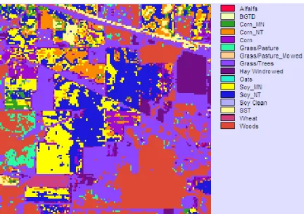
Figure 3.1 Indiana Pine hyperspectral image ... 53

Figure 3.2 Indiana Pine Ground truth & the labels ... 53

Figure 3.3: Hyperspectral image classification procedure ... 61

Fig 3.8: Hyperspectral image of Washington D. C. Mall ... 65

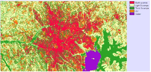
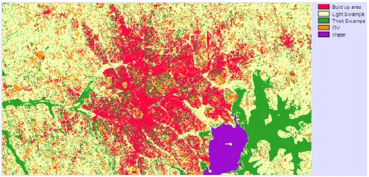
Figure 4.1: Map generated with BSI using 2 bands ... 73

Figure 4.2: Map generated with DSI using 2 bands ... 73

Figure 4.3: Map generated with TDSI using 2 bands ... 74

Figure 4.4: Land cover map obtained from an ensemble of 10 bands (Ensemble 1) . 77 Figure 4.5: Land cover map obtained from an ensemble of 14 bands (Ensemble 2) . 77 Figure 4.6: Land cover map obtained from an ensemble of 18 bands (Ensemble 3) . 78 Figure 4.7: Land cover map obtained from an ensemble of 18 bands ... 78

(16)

xvi

Figure 4.8: Graphical illustration of accuracy variation. ... 82

Figure 4.9: Ensemble made up of 4 bands classification Accuracy map ... 83

Figure 4.10: Ensemble made up of 6 bands classification Accuracy map ... 83

Figure 4.11: Purest pixels occur at the edges of the projected vector ... 89

Figure 4.12: Generated images and RMS error from PPI method ... 90

Fig 4.13: Purest pixels occur at the edges of the projected vector ... 101

Fig 4.14: Fraction images for each endmember ... 102

Map generated from accuracy result of Ensemble using BSI with 3 bands ... 135

Map generated from accuracy result of Ensemble using DSI with 3 bands ... 136

Map generated from accuracy result of Ensemble using TDSI with 3 bands ... 138

Map generated from accuracy result of Ensemble using NSM with 6 bands ... 139

Ensemble made up of 8 bands classification Accuracy map ... 140

(17)

xvii

LIST OF TABLES

Table 2.1: Hypothesis for diversity ... 35 Table 3.1. Number of pixels extracted from the ROI ... 63 Table 3.2: Number of pixels extracted from ROI ... 66 Table 4.1: Separability index classification results using Bhattacharyya distance ... 69 Table 4.2: Separability index classification results using divergence ... 69 Table 4.3: Separability index classification results using transformed divergence ... 70 Table 4.4: Ensemble using no Seperability measure ... 70 Table 4.5: Binomial Test of significance between ensembles ... 72 Table 4.6: Ensemble feature selection classification accuracy results ... 76 Table 4.7 Binomial Test of Significance between Majority Vote and Single Best .... 79 Table 4.8: Binomial tests of significance between the different ensembles based on majority vote values ... 80 Table 4.9: Binomial tests of significance between the different ensembles based on single best values ... 80 Table 4.10: Ensemble size classification Accuracy results ... 81 Table 4.11: Between-ensemble Binomial test of significance for 3 base classifiers .. 84 Table 4.12: Between-ensemble Binomial test of significance for 6 base classifiers .. 85 Table 4.13: Between-ensemble Binomial test of significance for 10 base classifiers 85 Table 4.14: Within-ensemble Binomial test of significance for 2 features ... 86 Table 4.15: Random selection ensemble accuracy results ... 87 Table 4.16: Between-ensemble Binomial test of significance for 3 base classifiers .. 88

(18)

xviii

Table 4.17: Between-ensemble Binomial test of significance for 9 base classifiers . 88

Table 4.18: Neural Network Confusion Matrix ... 91

Table 4.19: Support Vector Machines Confusion Matrix ... 92

Table 4.20: Random Forest Confusion Matrix ... 92

Table 4.21: C4.5 Confusion Matrix ... 93

Table 4.22: Bagging Confusion Matrix ... 93

Table 4.23: Spectral unmixing classification accuracy results ... 94

Table 4.24: Overall percentage accuracy results’ analysis of different classification schemes performance on the land cover classes ... 95

Table 4.25: Random forests error confusion matrix ... 103

Table 4.26: Neural networks error confusion matrix ... 104

(19)

xix

Nomenclature

AMEE: Automatic Morphological Endmember Extraction

ANC: Abundance Non-negativity Constraint

ASC: Abundance Sum-to-one Constraint

AVIRIS: Airborne Visible/Infrared Imaging Spectrometer

BSI: Bhattacharyya Separability Index

CVM: Cross Validation Majority

DSI: Divergence Separability Index

ENVI: Environment for Visualizing Images

GIS: Geographic Information Systems

GPS: Global Positioning Systems

GPUs: Graphics Processing Units

GRG: Generalized Reduced Gradient

HI: Hyperspectral Image

ISDAS (CCRS): Imaging Spectrometer Data Analysis System

ISIS Integrated Software for Imagers and Spectrometers

LARSYS: Laboratory of Applications of Remote Sensing Image Data

(20)

xx

LIBSVM: A Library for Support Vector Machines

LM: Landsat Thematic

LSMA: Linear Spectral Mixture Analysis

MNF: Maximum Noise Fraction

NN: Nearest Neighbour

NSM: No separability measure

PCA: Principal Component Analysis

PPI: Pixel Purity Index

RF: Random Forest

RMS: Root Mean Square

SI: Separability Index

SIPS (CU/CSES) Spectral Image Processing System

SPAM Spectral Analysis Manager

SVM: Support Vector Machines

TDSI: Transformed Divergence Separability Index

WEKA: Waikato Environment for Knowledge Analysis

(21)

1

CHAPTER 1 Introduction

1.1 Background of the study

Increasingly earth observation has become a prime source of data in the Geosciences and many related disciplines permitting research into the distant past, the present and into the future. Earth observation is based on the premise that information is available from the electromagnetic energy field arising from the earth’s surface or atmosphere (or both) and in particular from the spatial, spectral and temporal variations in that field (Levin, 1999; Kramer, 2002; Sabino, 2005). Through this, the environment can be better monitored, modelled, and consequently, better policy decisions made.

One of the areas of research interest has always been how to relate earth observation output e.g. Aerial photographs and satellite images (remotely sensed imagery) to known features (e.g. Land cover). Land cover refers to the physical surface of the earth, including various combinations of vegetation types, soils, exposed rocks and water bodies as well as anthropogenic elements, such as agriculture and built

environments (Mathur, 2004; Udelhoven, 2009; Sánchez et al., 2010). A land cover

map consists of a set of contiguous map units each of which is labelled according to a land cover class. The main reason for producing land cover maps is to give a clear idea of the stock, state of nature and built resources.

One critical environmental aspect to which satellite images can be applied is land cover mapping using classification algorithms called classifiers. An emerging area of

(22)

2

research interest relating image classification to land cover mapping is ensemble classification (Breiman, 1996; Kittler et al., 1998; Opitz, 1999; Giacinto and Roli,

2001; Polikar, 2006; Oza and Tumer, 2008; Marwala, 2009; Gidudu et al., 2009a).

Whereas previous research (Wacker and Landgrebe, 1972; Roli et al., 1997; Pinho et

al., 2008) has sought to find better classification algorithms, ensemble classification

is premised on using a ‘consensus’ approach to land cover mapping, the ‘consensus’ being dependent on a collection of base classifiers. Ongoing research in the application of ensemble classification to land cover mapping has focused on the

different ways ensembles can be constituted (Chen et al., 2007; Chan and Paelinckx,

2008; Udelhoven et al., 2009). Some of the common approaches (Breiman, 1996;

Opitz, 1999; Pal, 2003; Tsymbal, 2005; Polikar, 2006; Marwala, 2011) have involved constituting ensembles using different classification algorithms, constituting base classifiers from using different training data, or deriving base

classifiers using different band combinations (ensemble feature selection) (Gidudu et

al., 2008b).

Classifying and mapping vegetation is an important technical task for managing natural resources as vegetation provides a base for all living beings and plays an essential role in affecting global climate change, such as inﬂuencing terrestrial (carbon dioxide) CO2 (Xiao et al., 2004; Xie et al., 2008). But classification

accuracy poses serious challenge and this is due to, the design procedure of classifier, choice of training sets from dataset and information conveyed to the algorithm (Oza and Tumer, 2008). Statistical based classifiers have been successfully applied to multispectral data but are not effective for hyperspectral data (Hsu, 2007). The major reason is the fact that the number of spectral bands in hyperspectral data is too large, relative to the training samples. An effective way to solve this problem is

(23)

3

to reduce the dimension of the hyperspectral images. This can be done by extracting a number of salient features from the hyperspectral data (Keshava and Mustard, 2002; Su et al., 2008; Sánchez et al., 2010).

Furthermore, hyperspectral sensor uses many contiguous bands of high resolution, which covers the visible, near-infrared, and shortwave infrared spectral bands

(Adams and Smith, 1986; Vane et al., 1993; Lillesand and Kiefer, 1994; Nascimento,

2005). Information obtained from a particular pixel in a given hyperspectral band is a mixture of the energies scattered by the constituent substances in the respective pixel spatial coverage (Adams and Smith, 1986). According to Heinz and Chang (2001), Linear Spectral Mixture Analysis (LSMA) is a commonly accepted approach to mixed-pixel classification in remote sensing to estimate fractional abundance present in the image pixels. This study addresses the concerned issues for a remote sensing hyperspectral data and classification.

1.2 Problem statement

In remote sensing software, there are arrays of classifiers that can be used for image classification. Despite these arrays, knowing and understanding the correct classifier to use for a particular dataset remains a major challenge. Majority of preceding research has centred attention on developing classifiers that are better than existing ones (Steele and Patterson, 2001; Pal, 2007). Ensemble classification is an emerging approach to land cover mapping whereby the final classification output is a result of a ‘consensus’ of classifiers. Ensemble classification has been successfully deployed, but little has been done to systematically analyze the interplay between the ensemble size and the resulting classification accuracy. Hence, to date it has not been ascertained how many base classifiers an ensemble should have, or for a given

(24)

4

ensemble, how many features should the base classifiers have and the dependency of them on the data in question.

An ensemble system should consist of base classifiers which are diverse i.e. Classifiers whose decision boundaries err differently. Nevertheless, it is not established if there is any correlation between classification accuracy and diversity measures. Previous work relating ensemble classification to land cover mapping has focused on investigating how combining different classifiers impacts on

classification accuracy (Foody et al., 2007), how different types of ensembles can be

applied to land cover mapping (Pal, 2007) and also enforcing diversity through bagging for land cover mapping (Steele and Patterson, 2001). Kittler et al., (1998) developed a common theoretical framework and revealed that many available algorithms are developed to solve different problems of classification where all the pattern representations are jointly used to make decisions. In this research, the influence of ensemble classification on land cover classification accuracy was investigated.

Hyperspectral Imagery data provide ample spectral information to identify and distinguish spectrally unique materials. Therefore, the classification of the materials and classifier performance over the data is very crucial. While the general procedures (pre-processing and classiﬁcation) for hyperspectral images and multispectral images are the same, the processing of hyperspectral data remains a challenge. Especially, cost effective and computationally efﬁcient procedures are

required to process a large number of image bands (Varshney and Arora 2004; Xie et

(25)

5

A major problem with hyperspectral dataset is mixed pixels which are associated with the hyperspectral sensor used during sensing. Spectral mixture analysis provides an efficient mechanism for the interpretation and classification of remotely sensed

multidimensional imagery (Plaza et al., 2002; Iordache et al., 2011). In remote

sensing literature, a number of techniques have been developed for unconstrained, partially constrained and fully constrained linear spectral unmixing which can be computationally expensive (Sanchez et al., 2010; Iordache et al., 2011). For fully constrained linear spectral mixing analysis, two constraints are imposed. First, the sum of the abundance fractions of information present in an image pixel should be one. Secondly, these abundance fractions should be nonnegative. The first constraint can be easily solved while the second has not been fully solved because disparities can be experienced and the solution requires numerical approaches. For this purpose, an experimental comparison of supervised learning classifiers for land cover classification of hyperspectral imagery was investigated.

1.3 Aim and Objectives

The study investigates the influence of ensemble classification approach and spectral mixing problems associated with hyperspectral imagery for land cover classification accuracy.

The objectives are to investigate:

 Diversity through training a given classifier on different features and land

cover accuracy

 Interplay between the structure of ensemble and land cover classification

(26)

6

 Interplay between combination rules of the ensemble and land cover

classification accuracy

 Fully constrained spectral unmixing analysis for land cover classification.

The process involved;

 Data dimensionality reduction using the Eigenvalues and Maximum Noise

Factor (MNF)

 Separate noise from data

 Obtain spectral endmembers and their corresponding spectral signatures

 Obtain the best pure spectral pixels from the dataset using the Pixel Purity Index (PPI)

 Estimate fractional abundance in the dataset thereby obtaining the numeric

values for land cover classification

1.4 Contribution to knowledge

Several research studies have been reported in the remote sensing literature on different classification algorithms. The ensemble classification approach has been proven to yield favourable results compared to single systems for a broad range of applications (Polika, 2006). This research revealed that on combining classifiers in its application for land cover mapping, there is no significant benefit in having many base classifiers. In this study, three base classifiers were sufficient to give an accurate result (Gidudu et al., 2009a, Abe et al., 2010).

Reports in the remote sensing literature on how to quantify diversity in the ensemble classification has focus investigation on finding measures to build diverse ensemble systems (Kuncheva and Whitaker, 2003). This research revealed that diversity

(27)

7

measures do not provide an adequate means upon which to constitute ensembles for

land cover mapping (Gidudu et al., 2008a).

The major contribution to knowledge of the study is the introduction of Generalized Reduced Gradient (GRG), an optimization technique to estimate fractional abundance in hyperspectral image for land cover classification. From literature, a number of techniques have been developed for unconstrained, partially constrained and fully constrained linear spectral unmixing which can be computationally

expensive (Sanchez et al., 2010). For instance, quadratic programming has been

applied to impose abundance sum-to-one constraint (ASC) and abundance no-negativity constraint (ANC) to obtain fractional abundance, but the disadvantage is that the algorithms are computationally expensive (Boardman, 1995; Settle and Drake, 1993; Heinz and Chang, 2001).

The method used by (Heinz and Chang, 2001) likewise has the limitation of excessive computational complexity as the number of endmember increases. Another approach is the application of the least square method which cannot satisfy the ASC and ANC. If applied, the solved abundance fractions of the material signatures may be negative and their sum within an image pixel may not necessarily be one. Hence, the solutions are generally not optimal in terms of material quantification (Heinz and Chang, 2001; Sanchez, et al., 2011).

Introducing Generalized Reduced Gradient (GRG), an optimization technique with fully constraints algorithm in this study provides solution to the problems of estimating fractional abundance in hyperspectral image. The estimated numeric values obtained was successfully used for land cover classification using various classifiers and the classification accuracy results are remarkably good (Abe et al.,

(28)

8

2012). This is important for decision maker to consider tradeoff in accuracy and complexity of methods. In addition, the research permits the analysis of spatial dimension of land cover change and will contribute to the assessment of consequences of land cover change.

Another contribution to knowledge is the ability to successfully apply the GRG

algorithm on the Indian pine dataset (Abe et al., 2012). The GRG algorithm has been

able to solve the land-cover classification scenario associated with the Indian pine dataset which has been researched for a long time due to the problematic nature of

the dataset (Landgrebe, 1998; Plaza et al., 2008). The algorithm was successfully

applied to Washington DC mall hyperspectral dataset (Abe et al., 2012). The

research reveals that the GRG algorithm can be successfully applied to any type of data. Hence, ensemble classifiers improve predictive accuracy.

The research outputs have been able to produce nine publications to its credit. These include five international conference publications, two local conference publications, one published in the Computing Research Repository (CoRR), one submitted for

Journal publication and one Book Chapters. Abe et al., 2012 obtained a merit award

based on the reviewer reports and the score reports of the conference committee members during the conference period.

1.5 Scope of the Thesis

The techniques used in this work are made general and can be used for other applications, other than considered in this thesis. Land cover classification accuracy was investigated throughout this work, using various classification algorithms. According to Congalton and Green (2009), there are two types of map accuracy assessment. They are positional and thematic accuracy assessments. Positional

(29)

9

accuracy involves location of map features accuracy and measures the distance between the spatial feature on a map and its true location on the ground.

On the other hand, thematic accuracy assessment deals with the labels or attributes of the features in the ground truth or reference map. The accuracy assessment that was used for this study was based on thematic. This measures whether the mapped feature labels are different from the true feature label. The process includes; designing of the accuracy assessment sample, data collection for each sample and results’ analysis. The study areas used for the research are thematic Landsat imagery of Kampala, the capital of Uganda, Indiana pines and Washington DC mall hyperspectral datasets.

1.6 Thesis Layout

The remaining parts of the thesis are structured as follows:

Chapter 2 presents related theory on remote sensing and applications. It will also include a survey of work done using different classification algorithms as applied to remotely sensed imagery.

Chapter 3 contains different design methodology used for this study. There are six investigations described in the chapter with each investigation carried out in accordance with the objectives of the study.

Chapter 4 shows the results obtained from the investigations carried out in chapter 3. It also contains discussions on the results.

Chapter 5 summarises the major findings of this research and recommendations for further research directions are given.

(30)

10

Appendices: Appendix A presents the Land cover maps obtained using Kampala dataset; Appendix B contains Land cover maps generated using Indiana pine dataset.

List of Publications

From the thesis, the following papers were published:

1. Abe, B. T., Olugbara, O. O. and Marwala, T. (2014). “Experimental comparison

of support vector machines with random forest for hyperspectral imaging land

cover classification,” Journal of Earth System Science, Indian Academy of

Sciences(Accepted).

2. Abe, B. T., Olugbara, O. O. and Marwala, T. (2014). “Classification of

Hyperspectral image using Machine Learning Methods,” IAENG Transactions on

Engineering Technologies, Book Chapters of Springer, Lecture Notes in

Electrical Engineering, Volume 247, pp 555-569.

3. Abe, B. T. and Jordaan, J. (2013). “Hyperspectral Image classification based on

NMF features selection method,” Proceedings of SPIE, Vol. 9067, 90670N, SPIE

Digital Library.

4. Abe, B. T., Jordaan, J. and Marwala, T. (2013). “Ensemble classifier using GRG

algorithm for land cover classification,” Proceedings of SPIE, Vol. 9067,

90670O, SPIE Digital Library.

5. Abe, B. T., Olugbara, O. O. and Marwala, T. (2012). “Hyperspectral Image

Classification using Random Forest and Neural Network,” Lecture Notes in

Engineering and Computer Science: Proceedings of the World Congress on Engineering and Computer Science 2012, WCECS 2012, 24-26 October, San Francisco, USA, pp 522-527.

(31)

11

6. Abe, B., Gidudu, A. and Marwala, T. (2010). “Investigating the effect of

ensemble classification on remotely sensed data for land cover mapping,” In

Proceedings of 2009 IEEE International Geoscience & Remote Sensing Symposium Earth observation-Origins to Applications, Honolulu, USA, 23 –39 July, pp. 2832 – 2835.

7. Gidudu, A., Abe, B. and Marwala, T. (2009b). “Random Ensemble Feature

Selection for Land Cover Mapping,” In Proceedings of 2009 IEEE International

Geoscience & Remote Sensing Symposium Earth observation-Origins to Applications, Cape Town South Africa, 12 – 19 July, pp. 840 – 842.

8. Gidudu, A., Abe, B. and Marwala, T. (2009a). “Investigating the effect of

Ensemble Size on Classification Accuracy”, In Proceedings of the 2nd

International Conference on Earth Observation for Global Changes, (EOGC2009), Chengdu, China 25– 29 May, pp. 2195 – 2199.

9. Gidudu, A., Abe, B.T. and Marwala, T. (2008b). “Ensemble feature selection for

hyperspectral imagery”, In Proceedings of the 19th Annual Symposium of the

Pattern Recognition Association of South Africa, Cape Town, South Africa, 27 – 29 November, pp. 27-32.

10.Gidudu, A, Abe, B. and Marwala, T. (2008a). “Land Cover Mapping Using

(32)

12

CHAPTER 2 Related theory

This chapter presents a summary of remote sensing and the concept of hyperspectral images. Related theories on feature extraction and classification algorithms used in the study are undertaken.

2.1 Land cover

The dynamic and complex nature of environmental changes poses numerous challenges to human development. With increasing deforestation, industrialization, urbanization, mineral exploration among others, the price has been environmental degradation. Some of the long term consequences of environmental degradation have included: increased poverty, as well as climate change resulting in unexpected prolonged rains and droughts (Xiao et al., 2004; Xie et al., 2008). Some of the mitigation measures include environmental monitoring, environmental modelling and advocacy about the importance of the environment. Assessing and monitoring the state of the earth’s surface is a major requirement for global change research and has resulted into new clarity and better awareness of the earth’s dynamic nature (Lambin et al., 2001; Jung et al., 2006).

Land cover serves as a basic inventory of land resources for all levels of government,

environmental agencies, and private industries throughout the world. Land Cover is

characterized by a large variety of special distinct classes. The diagnosis and evaluation of the spectral separability measure yield the potential for automated

identification and mapping of these classes. Land cover mapping has found

(33)

13

series analysis, agricultural monitoring, natural resource monitoring, error assessment and uncertainty management among others (Bruzzone and Cossu, 2002;

Wolter, 2005; Randall, 2006; Chen et al., 2007; Xie, et al., 2008)

2.1.1 Why Land Cover mapping?

Land cover refers to the surface cover of the earth. Land cover mapping constitutes an integral component of the process of managing the land resources and mapped information is the result of analysis of remotely sensed data (Levin, 1999). According to Congalton and Green, (2009), because the earth’s resources are scarce, and more people are added to it continually, there will be a shortage of resources and their values. Hence, the need for timely and accurate information dissemination on the type, quantity and degree of resources increase. For this reason, land cover mapping is regarded as important for environmental management and land use policy making. Because of its broad coverage and cost-effectiveness, application of remote sensing to derive land cover information, using either manual interpretation or automated classification has been on the increase. The latter is frequently used as it rapidly reduces the workload of the image interpretation and requires much less expert knowledge (Zhou and Yang, 2009).

2.2 Remote sensing

Remote sensing is the acquisition and analysis of information about the earth from a distance using a computer and sensor through electromagnetic radiation. This started in 1830s with the origination of the camera (Jorgensen, 2004). Figure 2.1 shows the concept of remote sensing. The leap from manual aerial photographic interpretation to ‘automatic’ classification was inspired by the availability of experimental data in various bands in the mid 1960’s as a prelude to the launch of the Earth Resources

(34)

14

Technology Satellite (ERTS – which was later renamed Landsat 1) (Maul and Gordon, 1975). Landsat Thematic (TM), a moderate resolution scanner makes it possible to view the co-occurrence of different materials within the ground instantaneous field of view of urban areas that are characterized by a pattern of very heterogeneous patches. This necessitated the adoption of digital multivariate statistical methods for the extraction of land cover information (Landgrebe, 1997). The conservation, preservation and sustainable yield of natural resources are increasingly dependent upon remotely sensed data for inventory and monitoring of changes (Xie, et al., 2008). A suite of digital data, such as high resolution satellite images is currently available for this purpose. New technologies such as Image Processing (IP), GPS and GIS are being used to integrate and process these data. Digital image processing is extremely important in fully harnessing the information in high resolution satellite imagery data.

Figure 2.1: Concept of remote sensing (Landgrebe, 1998).

Remote sensing technology not only can be applied to map vegetation covers over land areas, but also in underwater areas with focus on mapping Submergent Aquatic

(35)

15

Vegetation (SAV), which is regarded as a powerful indicator of environmental

conditions in both marine and fresh water ecosystems (Wolter et al., 2005; Lathrop

et al., 2006; Xie et al., 2008).

2.3 Data collection

Remote sensing instruments, measures reflected electromagnetic radiation with the aid of aerial or satellite platform (Figure 2.2). Remotely sensed imageries are obtained using passive or active remote sensors. Passive sensors measure energy that is naturally available through sun ray when available, while active sensors depend on their energy source for illumination. Passive sensor can only be used during the day since that is when the sun is available to illuminate the earth. Active sensors radiate energy directly to the target object to be investigated. The sensor detects and measures the radiation reflected from that target.

Figure 2.2: Remote sensing sensors (Levin, 1999).

(36)

16

A remote sensing image is an objective recording of the electromagnetic reaching the sensor. The electromagnetic spectrum (figure 2.3) ranges from shorter wavelengths to the longer wavelengths. Though there are several regions of the spectrum that can be used for remote sensing, the most frequently used is the ultraviolet portion. The ultraviolet portion of the spectrum has the shortest wavelengths of the electromagnetic spectrum.

Figure 2.3: Electromagnetic spectrum (Levin, 1999)

The remote sensing process involves interaction between incident radiation and the targets of interest are as shown in figure 2.4. The radiation used for remote sensing travels through some distance through the atmosphere before reaching the earth to collect the information on the target. The seven stages comprising the process of remote sensing as shown in figure 2.4 are:

(37)

17

 Radiation and the atmosphere (B)

 Interaction with the target (C)

 Recording of energy by the sensor (D)

 Transmission, Reception and Processing (E)

 Interpretation and analysis (F)

 Application (G)

Figure 2.4: Remote Sensing process (Levin, 1999)

2.4 Image resolutions

Spectral resolution is the ability of a sensor to produce clear or distinguished wavelength interval, known as channels or bands in the electromagnetic spectrum (Fundamental of Remote Sensing). The arrangement of pixels in an image describes the spatial structure while radiometric describes the actual information contained in

B B C D E F G A

(38)

18

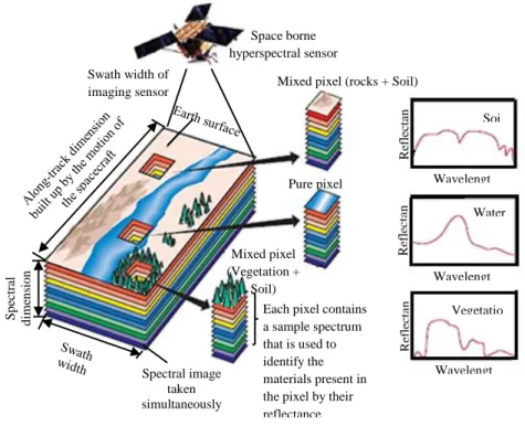
the image. The temporal resolution is the length of time taken by the satellite to complete one entire orbit cycle. The image obtained by remote sensors may contain one spectral band called panchromatic image (black and white), multispectral images contains few spectral bands and contiguous spectral bands are hyperspectral images. Different class labels and details in an image can be distinguished when their responses over a distinct wavelength range are compared (Fundamental of Remote Sensing). Figure 2.5 shows the three dimensional hyperspectral data cube and can be treated as a stack of two dimensional spatial images, each corresponding to a particular narrow spectral band.

Figure 2.5: Three dimensional hyperspectral data (Shaw and Burke, 2003)

2.5 Hyperspectral Imagery

Recent developments in sensor technology have resulted in the development of hyperspectral instruments. The instruments are capable of collecting hundreds of images (spectral bands) corresponding to wavelength channels, for the same area of the earth’s surface (Green et al., 1998; Plaza et al., 2003). Each pixel contains in

Soybean-notil Woods Grass/pasture Spatial dimension Corn-notill 100-220 spectral

(39)

19

hyperspectral data cube is linked to spectral signature or fingerprint that uniquely characterize the materials within the pixel (Figure 2.6). Such recognition provides a great advantage for detecting minerals, urban planning and vegetation studies, monitoring and management of environment, security and defense matters among

others (Varshney and Arora, 2004; Xie et al., 2008). However, accurate

classification of remote sensing images is an important task to be able to achieve

these advantages (Shaw and Burke, 2003). The existing classifiers are certainly

diverse, robust and powerful, it is abundantly clear that much information remains untapped in modern hyperspectral data, awaiting new algorithms and software implementations.

Figure 2.6: Concept of imaging Spectrometer (Shaw and Burke, 2003)

S p ec tr al d ime n si o n Spectral image taken simultaneously

Each pixel contains a sample spectrum that is used to identify the materials present in the pixel by their reflectance Mixed pixel (Vegetation +

Soil)

Pure pixel

Mixed pixel (rocks + Soil) Space borne hyperspectral sensor Swath width of imaging sensor R ef le ct an R ef le ct an R ef le ct an Vegetatio Water Soi Wavelengt Wavelengt Wavelengt

(40)

20

2.6 Spectral mixture

In hyperspectral imagery, a pixel is usually mixed with a number of materials present in the scene. Spectral mixture analysis has been extensively used in remote sensing for material discrimination, classification and detection. Various spectral mixture techniques have been reported in the remote sensing literature (Plaza et al., 2002;

Keshava and Mustard, 2002; Plaza et al., 2004b; Pinho et al., 2008; Zhang and

Huang, 2010). However, the spectral signature of a particular pixel contains a mixture of the signatures (fingerprints) of the numerous materials present within the spatial coverage of the target field view by the sensor. This is due to one of the following reasons:

(1) Low spatial resolution of the sensor used that distinct material can jointly

occupy one pixel. The outcome spectral measurement contains some composite of the individual spectral. This is common with remote sensing platforms operating at high altitude, covering large area surveillance with low spatial resolution.

(2) Mixed pixel can also occur when unique materials are combined into a

homogeneous mixture (Sanchez et al., 2010).

Spectral unmixing is the process whereby the measured spectrum of a mixed pixel is broken down into a number of pure spectral components, referred to as endmembers. This is also known as class labels, class types, components or signatures (Gong and Zhang 1999) and a set of corresponding fractional abundance that indicate the

amount of each endmember present in the pixel (Plaza et al., 2004b; Sanchez et al.,

2010). In hyperspectral imagery, linear spectral unmixing is a commonly accepted approach to mixed-pixel classification. Distinct substances such as water, tree, bridge, grass among others which are called the endmembers and the fraction in

(41)

21

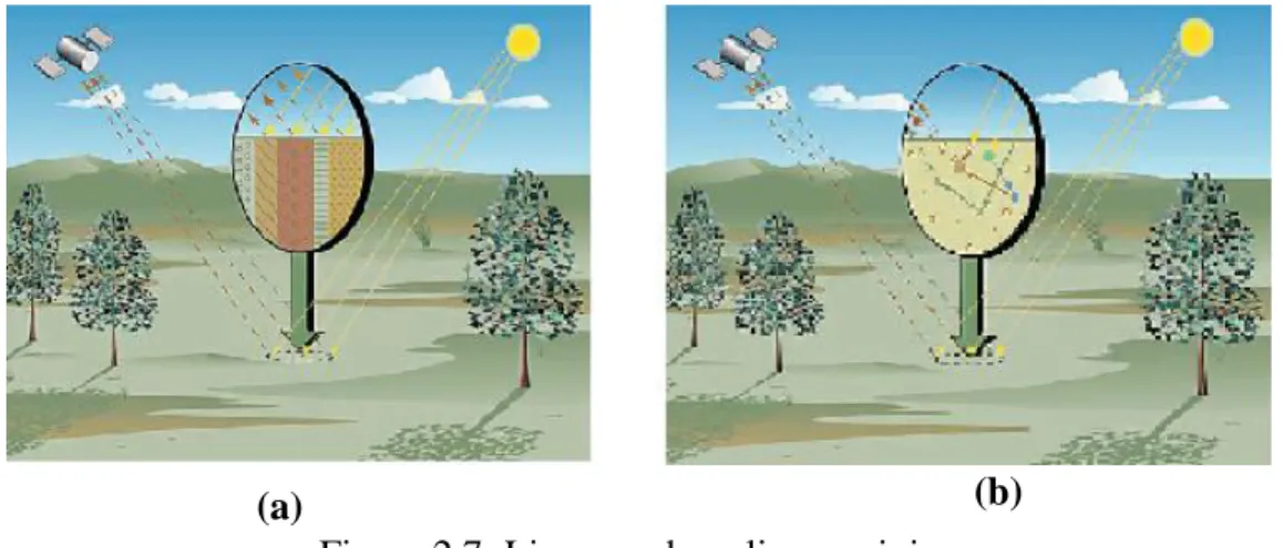
(a) (b)

which they emerge in the mixed pixel is referred to as fractional abundance. The other method used is the nonlinear mixing, where the incident sun ray comes across close mixture that causes multiple bounces.

The disadvantage of using nonlinear method is that the particle size, composition and altered state of the endmembers due to the multiple bounce significantly control the parameters of the solution (Keshava and Mustard, 2002). For experiment 5 of this research, linear unmixing method was adapted to generate fractional abundance in order to determine the degree of abundance in each endmember present in the pixel.

Figure 2.7: Linear and nonlinear mixing

(a) Linear mixing: Radiated sun reflected from the target through a single bounce (b) Nonlinear mixing: Radiated sun encounters an intimate mixture that stimulates multiple bounce (Keshava and Mustard, 2002).

We chose five algorithms from WEKA software for classification procedure because they are freely available and research has shown that the software has produced good results in remote sensing imagery classification (Garner, 1995; Pinho et al., 2008;

(42)

22

Random forest, Support vector machine, neural networks, bagging using REPtree as the base classifier. In the next session, some applications of these classifiers that were used in this research are discussed.

2.7 Image processing and classification

Image processing is any form of signal processing for which the input is an image, such as satellite images, a photograph or video frame. The output of image processing may be either image, a set of characteristics or parameters related to the image. Image processing is of interest because it affords abundant data to be translated into useful information in time (Liu et al., 2009). Numerous sources of imagery are identified by their differences in spectral, spatial, radioactive and temporal characteristics, hence are suitable for different purposes of vegetation mapping. Then, correlations of the vegetation types (communities or species) within the classiﬁcation system with discernible spectral characteristics of remote sensed imagery have to be identiﬁed. These spectral classes of the imagery are eventually translated into the vegetation types in the image interpretation process, which is also

called image processing (Xie et al., 2008).

The abilities to retrieve information from the data motivates researchers to explore methods of data mining, a non-trivial process of identifying valid, novel, potentially

useful, and ultimately understandable patterns in data (Fayyad et al., 1996; Xie et al.,

2008; Li, 2011). Increasingly Earth observation has become a prime source of data in

the Geosciences and many related disciplines permitting research into the distant past, the present and into the future. One of the areas of research interest has always been how to relate earth observation output e.g. Aerial photographs and satellite images (remotely sensed imagery) to known features. Pre-processing of remotely sensed (satellite) images prior to vegetation extraction is important to remove noise

(43)

23

and increase the interpretability of image data. This is true when dealing with time series of imagery or when an area is covered with many images since it is crucial to make these images compatible spatially and spectrally. It is expected that results obtained after image pre-processing should appear as if the image were acquired from the same sensor (Hall et al., 1991; Xie et al., 2008).

Image classification is the process whereby pixels in an image are automatically categorized into land cover classes. It is a fundamental analysis technique for remotely sensed data and involves the categorization of pixels based on their spectral characteristics (Cihlar et al., 1998). Image classification can be categorized into (i) supervised and unsupervised, (ii) Spectral and contextual classifications.

2.7.1 Supervised and unsupervised classification

Supervised classification requires the user to decide which classes exist in the image, and then delineate samples of these classes. These samples (known as training areas) are input into a classification program, which produces a classified image. The choice of the training area is based on the researcher’s familiarity with the geographical area and knowledge of the actual land cover types in the image. Unsupervised classification does not require training areas. Actually, it is the opposite of the supervised classification process. Spectral classes are grouped based significantly on the numerical information in the data and then matched by the researcher to the information classes (Bortolot, 1999; Sabino, 2005). Types of supervised classifiers include Minimum – Distance to Means, Neural Networks, and maximum likelihood classifiers, while examples of unsupervised classifiers include K – Mean, Fuzzy C means, and ISODATA among others (Bortolot, 1999; Sabino, 2005).

(44)

24

2.7.2 Spectral and contextual classifications

Spectral techniques are based on the spectral response pattern of a pixel and are divided into two categories, parametric and non-parametric classifiers. Parametric classifiers assume a Gaussian distribution of the data. In supervised parametric classification, a multivariate Gaussian distribution associated with each class is extracted from the training set by estimating the mean vector and the covariance matrix. Parametric classifiers are based on the definition of some discriminate functions based on the parameters of normal distribution. An example of parametric classifiers is a Gaussian maximum likelihood classifier. Non-parametric classifiers imply decision boundaries of arbitrary geometry and needs an iterative process to complete the boundaries. Example of these classifiers includes Nearest Neighbor (1-NN) 3, K-Nearest Neighbor (k-(1-NN) 4 techniques, kernel methods, and classification trees. Contextual classifiers consider the special context of a pixel in the image and are generally applied on remote sensing data when a large variety of spectral responses are observed in the same field. Contextual classifiers have been used successfully in a number of different problems such as coping with segmentation and classification of remotely sensed data (Dwivedi, et al., 2004).

2.8 Classifiers

This section presents a brief discussion on the classifiers used for this research. Supervised classification method was used for all the investigations carried out in the research.

2.8.1 Support Vector Machines (SVMs)

The construction of Support Vector Machines (SVMs) classifier has been described

(45)

25

Watanachaturaporn & Arora, 2004; Watanachaturaporn et al., 2004, Bruzzone et al.,

2006). The classifier has been proven to have a high generalized ability to solve classification problems and has been extensively used in supervised classification for

land cover mapping (Cortes and Vapnik, 1995; Lennon et al., 2002; Melgani and

Bruzzone, 2004; Gidudu, 2006; Abe et al., 2010). This technique has been used in

different application domains, including object detection and text categorization and has outperformed the traditional neural network technique in terms of generalization

capacity (Taratinno et al., 2006). It has a very interesting property for hyperspectral

image analysis in the sense that it does not suffer from Hughes phenomenon and with a small number of training samples it can separate classes easily (Cortes and

Vapnik, 1995; Lennon et al., 2002; Qi and Huang, 2007). SVM selects the optimal

hypothesis as the one yielding the maximum margin of separation between two classes (Vapnik, 1995). Among multi-class SVMs frequently used is one against one (1A1) algorithm, a type used in this research. The method constructs k (k – 1) /2 hyperplanes where each is trained on the data from two classes selected out of k classes. The performance and computation cost of (1A1) has been established, when compared with other SVM methods that no method can compete with one against one in terms of training and the good statistical performance. For a k-class problem, 1A1 algorithm creates all pairwise discriminating hyperplanes, in the sense that (k – 1) hyperplanes are created to separate one class from others. All final borderlines are

included in the created hyperplanes. The decision function for class ij is defined as

(46)

26    

_w

_b

f

ij ij ij x X   .  (2.1)

This is obtained by solving this optimization problem (Platt 2004):

  n ij n C ij w  2 2 1 min

 

_

 ij n ij ij n

w

b

x

.  1 , if

y

i n (2.2) Subject to:

 



 ij n ij ij n w b x .  1 , if

y

j, n (2.3) 0 



ij n

for all n examples in classes i and j. Given that

f

 

X 

f

  

X ,k k1



2

ij

ij diverse decision function for a k – class

problem exist. The 1A1 method used for class recognition in this research was the “max wins” algorithm. In this method, each classifier casts one vote for its chosen class and the class with majority vote wins. This means (Platt 2004):

Class X  arg maxi k sign

 

X

i

j

f

ij



1 (2.4)

Where sign (fij) represents the sign function, meaning that it has the value 1 when fij

(47)

27

unclassifiable region is given to the nearest neighbour applying real value decision functions as (Platt 2004):

Class X  arg maxi k

 

X

i

j

f

ij



1 (2.5)

The SVM used in this study experiment is the Gaussian kernel, which is Radial basis function (RBF) is given by (Platt 2004):



_x



_x

x

j K i j i 2 exp ,    (2.6) The network operates in a way that one basis function is centered on all training instances. The predicted outputs are combined linearly by computing the maximum margin hyperplane (Witten and Frank, 2005). The SVM (LIBSVM) used for sequential minimal optimization (Chang and Lin, 2001) in WEKA software was used for the classification.

2.8.2 Neural network

Neural network methods are general classifiers that can handle problems with lots of parameters and can classify objects, even when the distribution of object in n-dimensional parameter space is very complex. Research activities have established that neural networks are capable alternative to numerous conventional methods (Zhang, 2000, Benediktsson et al., 1990; Benediktsson and Swain, 1992, Marwala, 2010). They are data driven, self-adaptive technique that adjust themselves to data under investigation without any explicit specification of the functional or distributional form. They are also universal functional approximations that can approximate any function with arbitrary accuracy (Cybenko, 1989; Hornik, 1991;

(48)

28

Zhang, 2000). In addition, neural networks are nonlinear models that make them flexible in modelling real world complex relationships. Furthermore, they are capable of estimating the posterior capability that provides the basis for creating the classification rule and carrying out statistical analysis (Zhang, 2000; Richard and Lippman, 1991, Marwala, 2010). Various neural networks are available for classification purposes (Lippmann, 1989), but this paper focus on multilayer perceptron (MLP) that uses back propagation to classify instances. The nodes in the network are all sigmoid.

2.8.3 C4.5

The C4.5 for many years was the standard decision tree classification algorithm used in the machine learning and data mining communities. The algorithm creates decision tree classifier to predict membership cases of categorical dependent variable from measures on one or more variable. It uses information gain ration matrix for classification. C4.5 uses the significance of statistic of error to trim branches and uses probability weighting to deal with feature loss during the training period (Richard et al., 2006; Wang et al., 2008). The algorithm works in a way that each node of the decision tree matches an attribute and individual arc matches a value range of the attribute. The value of the expected attribute is known by the path from the root to individual leaf. The highest attribute is allocated to each node. This aims

at associating the attribute to reduce the data entropy to a node (Pinho et al., 2008;

Silva et al., 2008). Moore (2009) claimed that C4.5 is consistent and performs better

using large data. Using Remote Sensing (RS) data for classification, Yu and Ai (2009) implemented rough set and C4.5 algorithm. The classifier performs well on that particular data type. Polat and Gunes (2009) conducted investigation using ‘one against all method’ with C4.5. The experiment was conducted with Dermatology,

(49)

29

Image segmentation, Lymphography datasets. They were able to achieve very good accuracy against other algorithms. But nothing was said about time taking by the algorithm and other datasets. Efficiency of an algorithm also depends on the type of data used. Jiang and Yu (2009) suggested a hybrid algorithm based on outlier detection and C4.5. They used imbalance data and make it stable with the application of outlier detection using C4.5 algorithm. The experiment produced good accuracy as compared with other algorithm.

2.9 Ensemble classifier

Ensemble classifiers are essentially a multi-classifier system, implying that their functionality is dependent on a collection of classifiers – an ensemble of classifiers to get an accurate result (Foody et al., 2007). In literature, ensemble classification systems go by a variety of names, such as a mixture of experts and a committee of

classifiers (Marwala, 2001; Polikar, 2006; Gidudu et al., 2009; Marwala, 2009;

Marwala, 2011). Individual predictions of the ensemble members are typically

combined by weighted or unweighted voting to classify new data (Foody et al.,

2007; Qi and Huang, 2007; Marwala, 2011). Research has shown that ensemble generates better classification accuracy results than the individual classifier making

up the ensemble (Jimenez et al., 1999; Giacinto and Roli, 2001; Polikar, 2006; Pal,

2007). In remote sensing Giacinto and Roli, 1997; and Roli et al., (1997) report the

application of an ensemble of neural networks and the integration of classification results of different type of classifiers.

The main idea behind ensemble classification is that one is interested in taking advantage of various classifiers at their disposal to come up with a ‘consensus’ result. This is made possible by the following fundamental reasons (Dietterich, 2009):

(50)

30

(i) Statistical: This problem comes up due to the small amount of training

data available as compared to the size of the hypothesis space. By constructing an ensemble out of all of these accurate classifiers, the algorithm can “average” their votes and reduce the risk of choosing the wrong classifier.

(ii) Representational: In most applications of machine learning, the true

function cannot be represented by any of the hypotheses in the space.

(iii) Computational: Many learning algorithms work by performing some

form of local search that may get stuck in local optima. An ensemble constructed by running the local search from many different starting points may provide a better approximation to the true unknown function. These three fundamental issues are the three most important ways in which existing learning algorithms fail. Hence, ensemble methods have the promise of reducing (and perhaps even eliminating) these three key shortcomings of standard learning algorithms, than any of the individual classifiers.

The challenge at hand, involves deciding which classifiers to consider and how to combine their results. Polika (2006) affirmed that while the prediction of the ensemble may not be better than the best individual classifier in the ensemble, the method will surely minimize the overall risk of making a particularly poor choice. In another justification, Polika (2006) opine that ensemble method, handling large volume of data set by a single classifier will not be realistic. The best way to handle the data is to partition it into smaller subsets, train different classifiers with different partitions of data, and combine their predictions using an intelligent combination rule. The outcome often proves to be more efficient (Kittler, 1998; Polika; 2006).

(51)

31

From available literatures, Polkar, (2006) recommends that the constituent classifiers in the ensemble have different decision boundaries (that is diverse), because if identical there will be no gain in combining the classifiers (Shipp and Kuncheva, 2002). Diversity in ensemble systems has been more commonly explored by considering different classifiers, training a given classifier on different portions of the data, using a classifier with different parameter specifications and using different features. Diversity in ensemble systems is ensured by selecting base classifiers which err differently, since strategically combining these classifiers can reduce the total

error (Tsymbal et al., 2005; Parikh and Poikar, 2007; Oza and Tumer, 2008;

Marwala, 2011) as illustrated in Figure 2.8.

Figure 2.8: Graphical illustration of an Ensemble classifier system (Parikh and Polikar, 2007)

Ba n d 5 Band 1 Band 4 Ba n d 3 Ba n d 2 Band 1 Combination criteria 

Ensemble classifiers for land cover mapping