Forecasting stock returns: A comparison of five models

(1)

by

Vhahangwele Cedrick Ramuada

Thesis presented in partial fulfilment of the requirements

for the degree of Master of Science in Mathematics in the

Faculty of Science at Stellenbosch University

Supervisor: Prof. Jeff Sanders Co-supervisor: Prof. Ronald Becker

(2)

Declaration

By submitting this thesis electronically, I declare that the entirety of the work contained therein is my own, original work, that I am the sole author thereof (save to the extent explicitly otherwise stated), that reproduction and pub-lication thereof by Stellenbosch University will not infringe any third party rights and that I have not previously in its entirety or in part submitted it for obtaining any qualification.

December 2018

Date: . . . .

(3)

Abstract

Forecasting Stock Returns: A Comparison of Five Models

Vhahangwele Cedrick Ramuada

Department of Mathematical Sciences, University of Stellenbosch,

Private Bag X1, Matieland 7602, South Africa.

Thesis: MSc October 2018

Forecasting the movement of stock returns prices has been of interest to re-searches for many decades. Due to the complex and chaotic nature of the stock market, it has been difficult for researches to find a model which can be used to accurately predict the movement of stock returns prices. Many statistical models have been proposed for forecasting the direction of move-ment of stock returns prices. The objective of this study was to use ARMA-type models and an Artificial Intelligence Neural Network model to predict the direction of movement of stock returns prices of four JSE listed com-panies, namely, Netcare Group Ltd, Santam Ltd, Sanlam Group Ltd, and Nedbank Group. The models were assessed in terms of their ability to pre-dict whether the next day’s returns price will godown orup.

Four type models, namely, Maximum Likelihood, ARMA-State Space, ARMA-Metropolis Hastings, AR(3)-AVGARCH(1,1)-Student-t model and an Artificial Neural Network (ANN) model were implemented to try to predict the direction of movement of stock returns prices. Historical (past) stock returns prices were used to make inference about future direc-tional movement of stock returns prices. Empirical results show that the ARMA-Maximum Likelihood, ARMA-State Space, AR(3)-AVGARCH(1,1)-Student-t model, and Artificial Neural Network (ANN) models have a strong

(4)

ability to predict whether the next day’s returns price will go down or up

with acceptable accuracy. However, the ARMA-Metropolis Hastings model performed very poorly, its highest accuracy was a mere 68%. Overall, em-pirical results show that the Artificial Neural Network model was superior or outperformed all the ARMA-type models, the highest accuracy achieved by the model was 89%. The results of the Superior Ability Test also showed that the ANN model was indeed superior to the Box-Jenkins ARMA type models in at least 5 cases.

(5)

Uittreksel

Vooruitskatting van voorraadopbrengste :´ n Vergelyking

van vfy modelle

(“Forecasting Stock Returns: A Comparison of Five Models”)

Vhahangwele Cedrick Ramuada

Departement Wiskuudige Wetenskappe, Universiteit van Stellenbosch, Privaatsak X1, Matieland 7602, Suid Afrika.

Tesis: MSc Oktober 2018

Die voorspelling van die beweging van voorraad opbrengs pryse, is van groot belang vir navorsing vir dekades. As gevolg van die komplekse en chaotiese natuur van die aandele mark, dit mooilik vir navorsers om ´ n model te vind wat gebruik kan word om akkurate voorspelling van die be-weging van die voorraad opbrengs pryse te maak. Verskeie statistiese mo-delle is voorgestel om rigting van beweging te voorspel van die aandele op-brengs prys. Die doel van hierdie studie was om die ARMA- tipe model en ´ n “kunsmatige intelligensie neurale netwerk"(Artificial Intelligence Neu-ral Network) model te gebruik om die rigting van beweging van aandele obrengs prys van vier JSE genoteerde maatskappye te voorspel; naamlik, Netcare Group Ltd, Santam Ltd, Sanlam Group Ltd, and Nedbank Group. Die modelle is beoordeel in terme van hul vermoë om te voorspel of die volgende dag se pryse sal op of afwaarts gaan.

Vier tipe modelle, naamlik Maksimum Waarskynlikheid, ARMA-Staat Ruimte, ARMA- Metropolis Hastings, AR(3)-AVGARCH(1,1)-Student-t modelle en ´ n KunsmaAR(3)-AVGARCH(1,1)-Student-tige Neurale NeAR(3)-AVGARCH(1,1)-Student-twork (ArAR(3)-AVGARCH(1,1)-Student-tificial Neural NeAR(3)-AVGARCH(1,1)-Student-twork :

(6)

ANN) model is geimplementeer om die bewegingsrigting van aandele op-brengs pryse te voorspel. Historiese aandele pryse is gebruik om afleidings te maak oor toekomstige rigtingbewegings van aandele pryse.

Gebaseer op ondervinding die resulte bewys dat die ARMA-Maksimum Waarskynlikheid, ARMA-Staat Rruimte, AR(3)-AVGARCH(1,1)-Student-t Modelle en Kunsmatige Neutral Netwerk (ANN) modelle ´ n sterk vermöe het, om die volgende dag se obrengs pryse af of hoër te voorspel met aan-vaarbare akkuraatheid. Nietemin, die ARMA-Metropolis Hastings modelle het baie swak gevaar , die hoogste akkuraatheid was ´ n blote 68%. In die algemeen, gebaseer op ondervinding die resultate wys dat die ANN model beter was en die ARMA-tipe modelle geklop het, die hoogste akkuraatheid behaal van die model was 89%. Die resultate van die Superior Ability Test het aangetoon dat die ANN model beter was as die Box-Jenkins ARMA-tipe modelle in ten minste 5 gevalle.

(7)

Acknowledgements

Firstly i would like to thank my supervisor Prof Ronnie Becker for his excel-lent guidance, insightful comments, patience, and encouragement through-out the duration of the study.

I would also like to thank the African Institute for Mathematical Sciences (AIMS) for providing funding for this study. To my colleagues, family and friends, thank you for your support.

(8)

Dedications

To my parents, Daniel and Itani Ramuada

(9)

List of Figures

3.1 A biological neuron (Raschka, 2015, p.18) . . . 42

3.2 Concept of perceptron (Raschka, 2015, p.24) . . . 43

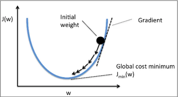
3.3 Gradient descent (climbing down a hill) (Raschka, 2015, p.35) . . . . 44

3.4 Concept of Multilayer Perceptron (MLP) (Raschka and Mirjalili, 2017, p.548) . . . 47

3.5 Backpropagation (Raschka and Mirjalili, 2017, p.586) . . . 49

5.1 Daily closing prices series of JSE listed companies . . . 63

5.2 Log returns series of JSE listed companies . . . 64

5.3 Summary results of ARMA(1,1) fit on Netcare returns series . . 67

5.4 Summary results of ARMA(1,1) fit on Sanlam returns series . . 68

5.5 Summary results of ARMA(1,1) fit on Santam return series . . . 69

5.6 Summary results of ARMA(1,1) fit on Nedbank returns series . 70 5.7 ACF plot of residuals of ARMA(1,1) model fitted on Netcare returns series . . . 71

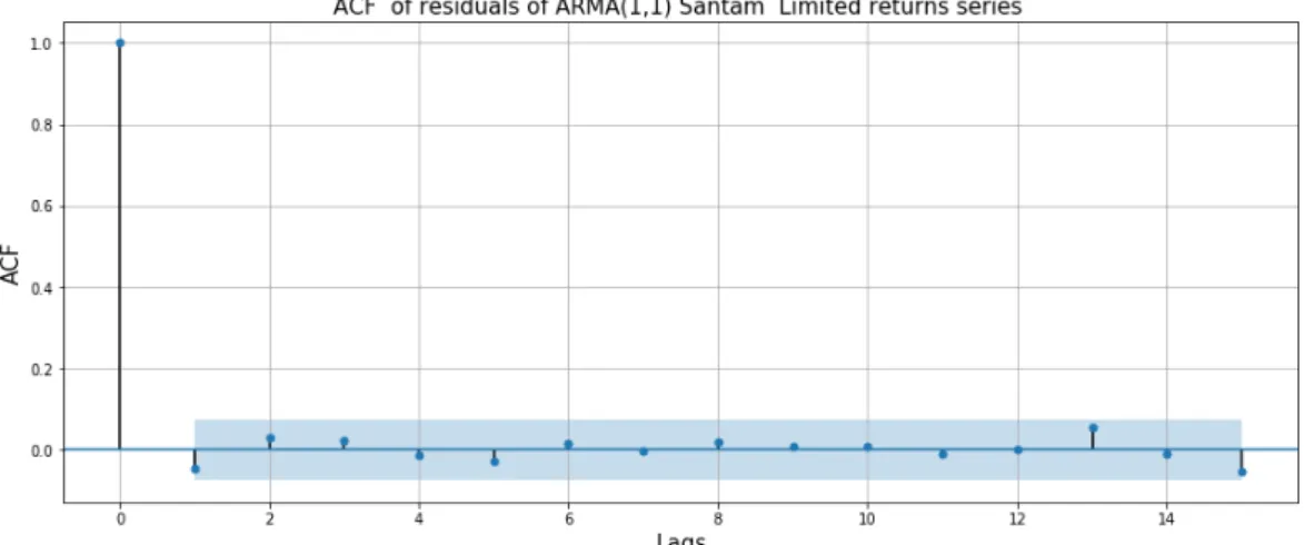
5.8 ACF plot of residuals of ARMA(1,1) model fitted on Santam returns series . . . 71

5.9 ACF plot of residuals of ARMA(1,1) model fitted on Nedbank returns series . . . 72

5.10 ACF plot of residuals of ARMA(1,1) model fitted on Sanlam returns series . . . 72

5.11 Histograms of residuals from the ARMA(1,1) models . . . 75

5.12 Daily returns series predictions using ARMA(1,1) model . . . . 77

5.13 Daily returns series predictions using ARMA(1,1) model . . . . 78

5.14 Summary results of the estimated AR(3)-AVGARCH(1,1)-Student-t model fiAR(3)-AVGARCH(1,1)-Student-t on NeAR(3)-AVGARCH(1,1)-Student-tcare reAR(3)-AVGARCH(1,1)-Student-turns series . . . 82

5.15 Netcare Group Ltd returns series predictions using AR(3)-AVGARCH(1,1)-Student-t model . . . 84

(13)

5.16 Summary results of the estimated AR(3)-AVGARCH(1,1)-Student-t model fiAR(3)-AVGARCH(1,1)-Student-t on SanAR(3)-AVGARCH(1,1)-Student-tam group reAR(3)-AVGARCH(1,1)-Student-turns series . . . 85 5.17 Santam Group returns series predictions using

AR(3)-AVGARCH(1,1)-Student-t model . . . 87 5.18 Summary results of the estimated

AR(3)-AVGARCH(1,1)-Student-t model fiAR(3)-AVGARCH(1,1)-Student-t on Sanlam group reAR(3)-AVGARCH(1,1)-Student-turns series . . . 88 5.19 Sanlam Group Ltd returns series predictions using

AR(3)-AVGARCH(1,1)-Student-t fiAR(3)-AVGARCH(1,1)-Student-t on Nedbank group reAR(3)-AVGARCH(1,1)-Student-turns series . . . 91 5.21 Nedbank Group Ltd returns series predictions using

AR(3)-AVGARCH(1,1)-Student-t model. . . 93 5.22 Summary results of State Space ARMA(1,1) model fit on

Net-care Limited Group returns series . . . 95 5.23 Netcare Group Ltd returns series predictions using State Space

ARMA(1,1) model . . . 96 5.24 Summary results of State Space ARMA(1,1) fit on Santam

Lim-ited returns series . . . 97 5.25 Santam Group returns series predictions using State Space ARMA(1,1)

model . . . 98 5.26 Summary results of the State Space ARMA(1,1) model fit on

Sanlam Group Limited returns series . . . 99 5.27 Sanlam Group Ltd returns series predictions using State Space

ARMA(1,1) model . . . 100 5.28 Summary results of State Space ARMA(1,1) fit on Nedbank

Group Ltd returns series. . . 101 5.29 Nedbank Group Ltd returns series predictions using State Space

ARMA(1,1) model . . . 102 5.30 Summary results of ARMA(1,1) Metropolis Hastings model fit

on Netcare Group Limited returns series . . . 104 5.31 Netcare Group Ltd returns series predictions using

ARMA(1,1)-MH model . . . 105 5.32 Summary results of ARMA(1,1) Metropolis Hastings model fit

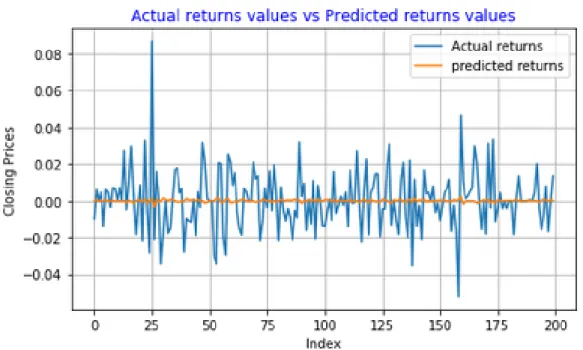
on Santam Ltd returns series . . . 107 5.33 Santam Ltd returns series predictions using ARMA(1,1)-MH

(14)

5.34 Summary results of ARMA(1,1) Metropolis Hastings model fit on Sanlam Group Ltd returns series . . . 109 5.35 Sanlam Group Ltd returns series predictions using

ARMA(1,1)-MH model . . . 110 5.36 Summary results of ARMA(1,1) Metropolis Hastings model fit

on Nedbank Group Ltd returns series . . . 111 5.37 Nedbank Group Ltd returns series predictions using

ARMA(1,1)-MH model . . . 112 5.38 Netcare Group Ltd returns series predictions using ANN model 114 5.39 Santam Ltd returns series predictions using ANN model . . . . 115 5.40 Sanlam Group Ltd returns series predictions using ANN model 116 5.41 Nedbank Group Ltd returns series predictions using ANN model117 5.42 Summary results of ARMA(1,1) model fit on Netcare returns

series . . . 120 5.43 ACF of residuals of ARMA(1,1) model fitted on Netcare returns

series . . . 121 5.44 Histogram of residuals of ARMA(1,1) model fitted on Netcare

Group Ltd returns series. . . 122 5.45 Netcare Group Ltd returns series predictions using ARMA(1,1)

model . . . 123 5.46 Summary results of ARMA(1,1) model fit on Santam Ltd

re-turns series . . . 124 5.47 ACF of residuals of ARMA(1,1) model fitted on Santam returns

series . . . 125 5.48 Histogram of residuals of the ARMA(1,1) model fitted on

San-tam Ltd returns series . . . 126 5.49 Santam Ltd returns series predictions using ARMA(1,1) model. 127 5.50 Summary results of the ARMA(1,1) model fit on Sanlam Group

Ltd returns series . . . 128 5.51 ACF of residuals from the ARMA(1,1) model fitted on Sanlam

returns series . . . 129 5.52 Histogram of residuals of ARMA(1,1) model fitted on Sanlam

Group Ltd returns series. . . 130 5.53 Sanlam Group Ltd returns series predictions using ARMA(1,1)

(15)

5.54 Summary results of ARMA(1,1) model fit on Nedbank Group Ltd returns series . . . 132 5.55 ACF of residuals from the ARMA(1,1) fitted on Nedbank

re-turns series . . . 133 5.56 Histogram of residuals of ARMA(1,1) model fitted on Nedbank

Group Ltd returns series. . . 134 5.57 Nedbank Group Ltd returns series predictions using ARMA(1,1)

model . . . 135 5.58 Summary results of the estimated

AR(3)-AVGARCH(1,1)-Student-t model fiAR(3)-AVGARCH(1,1)-Student-tAR(3)-AVGARCH(1,1)-Student-ted on NeAR(3)-AVGARCH(1,1)-Student-tcare reAR(3)-AVGARCH(1,1)-Student-turns series . . . 138 5.59 Netcare Group Ltd returns series predictions using the

AR(3)-AVGARCH(1,1)-Student-t model. . . 140 5.60 Summary results of the estimated

AR(3)-AVGARCH(1,1)-Student-t model fiAR(3)-AVGARCH(1,1)-Student-tAR(3)-AVGARCH(1,1)-Student-ted on SanAR(3)-AVGARCH(1,1)-Student-tam reAR(3)-AVGARCH(1,1)-Student-turns series . . . 141 5.61 Santam Ltd returns series predictions using

AR(3)-AVGARCH(1,1)-Student-t model fiAR(3)-AVGARCH(1,1)-Student-tAR(3)-AVGARCH(1,1)-Student-ted on Sanlam reAR(3)-AVGARCH(1,1)-Student-turns series . . . 144 5.63 Sanlam Group Ltd returns series predictions using

AR(3)-AVGARCH(1,1)-Student-t model fiAR(3)-AVGARCH(1,1)-Student-tAR(3)-AVGARCH(1,1)-Student-ted on Nedbank reAR(3)-AVGARCH(1,1)-Student-turns series . . . 147 5.65 Nedbank Group Ltd returns series predictions using

AR(3)-AVGARCH(1,1)-Student-t model. . . 149 5.66 Summary results of the State Space ARMA(1,1) fitted on

Net-care Group Ltd returns series . . . 152 5.67 Netcare Group Ltd returns series predictions using the State

Space ARMA(1,1) model . . . 153 5.68 Summary results of the State space ARMA(1,1) model fitted on

Santam Ltd returns series . . . 154 5.69 Santam Ltd returns series predictions using State Space ARMA(1,1)

model . . . 155 5.70 Summary results of State Space ARMA(1,1) model fit on

San-lam Group Ltd returns series . . . 156 5.71 Sanlam Group Ltd returns series predictions using State Space

(16)

5.72 Summary results of State Space ARMA(1,1) model fitted on Nedbank Group Ltd returns series. . . 158 5.73 Nedbank Group Ltd returns series predictions using State Space

ARMA(1,1) model . . . 159 5.74 Summary results of ARMA(1,1)- Metropolis Hastings model

fitted on Netcare Group Limited returns series . . . 161 5.75 Netcare Group Ltd returns series predictions using

ARMA(1,1)-MH model . . . 162 5.76 Summary results of the ARMA(1,1) Metropolis Hastings model

fitted on Santam Ltd returns series . . . 163 5.77 Santam Ltd returns series predictions using ARMA(1,1)-MH

model . . . 164 5.78 Summary results of ARMA(1,1) Metropolis Hastings model

fit-ted on Santam Group Ltd returns series. . . 165 5.79 Sanlam Group Ltd returns series predictions using

ARMA(1,1)-MH model . . . 166 5.80 Summary results of ARMA(1,1) Metropolis Hastings model

fit-ted on Nedbank Group Ltd returns series . . . 167 5.81 Nedbank Group Ltd returns series predictions using

ARMA(1,1)-MH model . . . 168 5.82 Netcare Group Ltd returns series predictions using ANN model 169 5.83 Santam Ltd returns series predictions using ANN model . . . . 170 5.84 Sanlam Group Ltd returns series predictions using ANN model 172 5.85 Nedbank Group Ltd returns series predictions using ANN model173

(17)

Nomenclature

ADF Augumented Dickey Fuller

ANN Artificial Neural Network

ARMA Autoregressive Moving Average

ARIMA Autoregressive Integrated Moving Average

ARCH Autoregressive Conditional Heteroscedasticity

DW Durbin Watson

EWMA Exponential Weighted Moving Average

JSE Johannesburg Stock Exchange

LM Lagrange Multiplier

MA Moving Average

MCMC Markov Chain Monte Carlo

MCSE Markov Chain Standard Error

MH Metropolis Hastings

MLP Multilayer Perceptron

PP Phillips Perron

SPA Superior Predictive Ability

(18)

Chapter 1 Introduction

Forecasting of stock prices is one of the most important topics in academic and financial studies. However, the stock market prices can be influenced by many factors such as political situations, economic events, and natural disasters etc. As a result, forecasting stock prices is a challenging task due to the complexity of the stock market. Financial time series forecasting in-volves trying to understand the data generation process using historic (past) observations and applying a chosen model to try to extrapolate the returns series into the future (Tang et al., 2003).

Many studies has been carried out to find the best models for forecasting stock prices. Two of the most popular categories for modelling time series are linear models e.g ARMA Models, and Exponential smoothing. The sec-ond category is nonlinear models (artificial intelligence based models) e.g Support Vector Machines, Genetic Algorithms, and Artificial Neural Net-works. The most popular of the linear models is the ARMA model first developed by Box-Jenkins in 1976. The ARMA model is widely used in financial time series forecasting because its quite flexible as it is made up of a combination of different types of time series models, namely, the Au-toregressive (AR) and the Moving Average (MA) model, hence the name Autoregressive Moving Average (ARMA).

However, many financial time series studies carried out have shown that there is little evidence that the stock market is perfectly linear. To deal with this problem, mixture models have been proposed. The most popular mix-ture model is the combination of ARMA models together with non-linear

(19)

models such as Autoregressive Conditional Heteroscedasticty (ARCH) and the Generalised Autoregressive Conditional Heteroscedasticty (GARCH). The ARMA-GARCH types models have been successfully used for fore-casting of financial time series (Majumder and Hussian, 2007). The ARCH model was first introduced by Robert F. Engle and Clive W. Granger in 1982 to model time varying volatility. Engle and Granger were awarded the No-bel prize for Economics in 2003 for this work. In 1986, Bollerslev introduced the Generalised ARCH model. The Generalised ARCH model is simply an extension of the ARCH model.

The rise in computer power, the availability of large amount of data, and advancements made in neural network theory has lead to a wide use of Ar-tificial Neural Networks (ANN) in financial literature. The main advantage of using ANN in predicting stock returns is their ability to find non-linear relationships in the data (Majumder and Hussian, 2007, p.3). ANN are used to overcome the drawbacks of linear models. Another advantage of ANN is that they can use non-linear activation functions such as the sigmoid, and tangent sigmoid which are able to detect non-linear patterns in a data set. As a result, accuracy of predictions can be improved by using these non-linear models (Majumder and Hussian, 2007),(Rather, 2014). Because of the chaos and complex nature of the system, traditional statistical models sometimes tend to be inadequate to understand the relationship between input data and output of the particular system. Artificial Neural Networks models are data driven, they do not require any prior assumption about the knowledge of the relationship that may exist between input and output of the system. Some researchers claim that the stock market behaves like a chaotic system. Neural networks have been widely used to model these chaotic systems because they have few assumptions about dynamic depen-dencies.

1.1 Aim of the Study

The aim of this project is to predict the financial log-returns of Johannes-burg Stock Exchange (JSE) listed companies. We will use Autoregressive Moving Average model, State Space ARMA Model, Autoregressive Moving Average model with parameters estimated through the Metropolis Hastings

(20)

algorithm, Autoregressive GARCH type models, and an Artificial Neural Network to make predictions. We will then evaluate each of the model in terms of how good it can predict whether the next day’s returns price will goupordown. The results will then be summarised using a confusion ma-trix. The Superior Predictive Ability (SPA) test will be used to determine the “best” model for predicting the direction of change of stock returns prices.

1.2 Research Objectives

Time series models and computational intelligence techniques have been widely used for forecasting of stock returns. However, few studies have been carried out to try to forecast the returns of emerging market such as the South African Market the JSE. Hence, the first objective of this project is to use ARMA-Metropolis Hastings algorithm, ARMA Maximum Like-lihood, State Space ARMA, AR-GARCH-type, and Artificial Neural Net-works models to forecast the log returns of JSE listed companies. The second objective is to assess whether the proposed models are able to accurately predict whether the next day’s returns price will go downorup. The third objective would be to identify the best model for forecasting log returns of the JSE listed companies.

1.3 Significance of the Study

During periods of economic instability or financial market turmoil, investors can suffer huge losses. As a result, prediction of the direction of movement of stock returns has gained more attention in recent times, this is because if we can successfully predict direction of movement of stock returns, then investors can be able to make profits from trading and investing in the stock market. If a system can be developed to predict movements and trends of stock market, then the owner of such a system would be wealthy. As a re-sult, findings emerging from this study will help investors to minimise risk to their portfolios, regulators in policy making, and hedge fund managers.

(21)

1.4 Structure of the Thesis

The structure of the research project is as follows: Chapter 2 reviews previ-ous literature on forecasting stock returns. Chapter 3 gives a introduction to statistical models to be used in the study. In Chapter 4, we discuss the meth-ods used for analysis, in Chapter 5 results are discussed. Finally in Chapter 6, we draw conclusion and also propose future work which may be carried out.

(22)

Chapter 2 Literature Review

In this chapter, we review some literature on stock returns forecasting. We will also review some of the models used in our study to see how well they performed when applied to different stock exchanges.

2.1 Studies on Forecasting Stock Returns Using

Time Series and Computational Intelligence

Models

A study was carried out by (Hansson, 2017) in an effort to forecast the log returns series using data from three stock markets the S&P 500, Bovespa (Brazil), and OMX 30 (Sweden). Two models used in the study for fore-casting the log returns were the ARMA(1,1)-GJRGARCH(1,1) and the Long Short Term Memory (LSTM). Results emerging from the study showed that both the ARMA(1,1)-GJRGARCH(1,1) and the LSTM achieves similar re-sults when regression approach is taken. But, the LSTM outperformed the ARMA(1,1)-GJRGARCH(1,1) in terms of prediction of direction of change for only the small Swedish market.

In their study, (Ferenstein and Gasowski, 2004b) used the AR(1)-GARCH types models to predict the stock returns prices of two companies from the Warsaw stock exchange. Results emerging from the study showed that the

(23)

AR(1)-GARCH(1,1) model outperformed the AR(1)-EGARCH model. The results showed that the AR(1)-GARCH(1,1) had the lowest Mean Squared Error (MSE) out of all models considered in the study.

The ARIMA-EGARCH model was used by (Hossain et al., 2015) to model stock volume data of the Dhaka Stock Exchange (DSH). Results from the study showed that the ARIMA-EGARCH model was able to forecast the stock volume series, with the model producing low Mean Absolute Error (MAE) and Mean Squared Error (MSE).

A study was carried out by (Majumder and Hussian, 2007), In an effort to try to predict the direction of the movement of the stock returns of the S&P 500, CNX 500, and NIFTY index using ANN based models. In their study, various features of the data and structures of the ANN model were used to predict direction of stock returns. Results emerging from the study showed that in terms of direction of price movements, the highest accuracy achieved by ANN was 89%, and an average of 69.72% was achieved for all different structures of ANN models.

(24)

Chapter 3 ARMA-Type Time Series and

Artificial Intelligence Techniques

In this chapter, statistical properties of log returns will be discussed. We will also discuss the models to be used in the study, this include the assumptions and parameter estimation methods for these models.

3.1 Financial Log Returns

Instead of using prices of assets, most financial studies uses returns (Tsay, 2005, p.2). (Campbell et al., 1997) specified two major reasons for using the returns

• Asset returns have attractive statistical properties. As a result, they are easier to handle than actual prices series.

• For a typical average investor, returns are a scale free and complete summary of an investment opportunity (Tsay, 2005, p.2).

The financial log returns are given as

rt =log Pt Pt−1 , (3.1)

where Pt is the closing price at timet, andrtare the log returns.

3.1.1 Statistical Properties of Financial Asset Returns

Financial log returns often exhibit the following statistical properties (Fry-zlewicz, 2005, p.1-2).

(25)

• The expected value of the returns sample is close tozero.

• The returns have a distribution with heavy tails (higher kurtosis). • They exhibits volatility clustering. That is, period of large changes in

the price of a financial asset tend to be followed by period of large changes, and also period of small changes tend to be followed by pe-riod of small changes (Rachev et al., 2008, p.185).

• The Autocorrelations for the sample are relatively small for almost all the lags.

Weakly Stationary

Suppose rt is a time series, then this time series is said to be weakly

sta-tionary if its long term expected value (mean) and variance converge to a constant as time goes to infinity (t → ∞). Weakly stationary simply means that data points of the series fluctuate around a fixed level (Tsay, 2005, p.29-30). Under weakly stationary, we assume that the first moment (mean) and the second moment ofrt are finite. In statistical finance literature, asset

re-turns series are usually assumed to be weakly stationary (Tsay, 2005, p.30).

White Noise

A time seriesrtis said to be Gaussian White noise if it has a mean ofzeroand

a constant variance, thus E(rt) =0 andvar(rt) = σ2. This can be expressed

mathematically as{rt} ∼W N(µ =0,σ2)(Tsay, 2005, p.36).

3.2 AutoRegressive (AR) Model

A simple AR(1) model is given as (Tsay, 2005, p.37-38)

rt =φ0+φ1rt−1+et, (3.2)

where rt−1 is the returns price at previous stept−1, et is a white noise

se-ries, andφ0,φ1are the model parameters which will be estimated using the

maximum likelihood approach (mle). The white noise serieset is

(26)

3.2.1 Statistical Properties of the AR Model

Below we will discuss the statistical properties of AR(1) model, AR(2) model and then proceed to give a generalization of the results of the general AR(p) model. If we assume that the time series rt is weakly stationary, then from

the properties discussed earlier it follows that E(rt)=µ and var(rt)=ρ (Tsay,

2005, p.38)

Proof:

E(rt) = E(φ0+φ1rt−1+et)

=φ0+φ1E(rt−1).

(3.3) But, under the stationary assumption we have that E(rt)=E(rt−1)=µ (Tsay,

2005, p.38-39). Therefore, according to (Tsay, 2005, p.38)

E(rt) =φ0+φ1E(rt−1) µ=φ0+φ1E(rt−1) µ=φ0+φ1µ E(rt) = µ= φ0 (1−φ1) . (3.4)

The above results implies that the expected value of rt exists if φ1 6=1, and E(rt) =0 ifφ0 =0.

Sinceµ = ₁₋φ0_φ

1 =⇒φ0=µ(1−φ1), then we can rewrite the AR(1) model as

(Tsay, 2005, p.38)

rt =φ0+φ1rt−1+et

rt =µ(1−φ1) +φ1rt−1+et

rt−µ =φ1(rt−1−µ) +et.

(3.5)

To find the variance, we take the square of the results above and apply the expected value (Tsay, 2005, p.38-39).

r2_t −µ2 =φ2₁(rt−1−µ)2+e2t (3.6)

E(r2t)−µ2=φ21E(rt−1−µ)2+E(e2t). (3.7)

(3.8) But, we know that var(rt)=E(r2t)−µ2, var(rt−1)=E(r2t−1)−µ2, and E(e2t)=σe2.

Therefore,

var(rt) =φ2₁var(rt−1) +σ_e2. (3.9)

(27)

But, under stationary assumption it is known that var(rt)=var(rt−1) (Tsay, 2005, p.39). Therefore, var(rt) = φ₁2var(rt−1) +σ_e2 var(rt)−φ₁2var(rt) = σe2 var(rt) = σ 2 e 1−φ2₁, φ 2 1 <1. (3.11)

The condition that φ₁2 < 1 is to ensure that the variance is non-negative.

Consequently, by definition of weakly stationary of AR(1) model we have that −1 < φ1 < 1. Therefore, the necessary condition required for

Autore-gressive model of order 1 to be weakly stationary is| φ1 |<1 (Tsay, 2005, p.

39). For more details about the proof see (Tsay, 2005, p.37-39).

AR(2) Model

Lemma: The AR(2) model is weakly stationary if the roots x1,x2 of x2−

φ1x−φ2 =0 satisfy | x1 |< 1 (i=1,2) and| φ1 | + | φ2 |< 1. The long term

mean

µ = lim

t→∞E(rt) and the long term variance

ρ= lim t→∞var(rt) are given by E(rt) = µ = φ0 (1−(φ1+φ2)) (3.12) and var(rt) = ρ= σ 2 e (1−(φ2₁+φ2₂)). (3.13)

The results above implies that the variance of return seriesrt exists ifφ₁2+ φ2₂ 6=1.

Proof: Weakly stationary can be proved similarly to the AR(1) case by using the variation of constants formula forrt. We omit this portion of proof.

(28)

AR(p) Model

The AR(p) model is a generalization of AR(1) model. It is given as (Tsay, 2005, p.46)

rt =φ0+φ1rt−1+φ2rt−2+· · ·+φprt−p+et, (3.14)

whereetis the white noise process,φ0is the model constant, andφ0,φ1,· · · ,φp

are the model parameters which are estimated using the maximum likeli-hood method. Applying the same techniques as that of AR(1), and AR(2) cases we have that (Tsay, 2005, p.46)

E(rt) = µ = φ0 1−(φ1+φ2+,· · · ,+φp) (3.15) and var(rt) = σ 2 e 1−(φ1+φ2+,· · · ,+φp). (3.16)

For a detailed explanation of Autoregressive models see (Tsay, 2005, p.36-47).

3.3 Moving Average (MA) Model

The MA model is a finite linear combination of the residuals et. In many

statistical finance literature, the MA model is simply known as the extension of the white noise series (Tsay, 2005, p.57). The MA(1) model is given as (Tsay, 2005, p.57-58)

rt =c0+et−θ1et−1, (3.17)

where et iid∼ N(0,σe2), this implies that et are independent and identically

distributed, each with a gaussian distribution with mean ofzeroand a con-stant variance, andc0is the model constant.

3.3.1 Statistical Properties of the MA Model

The first and second moment ofrt are time invariant, therefore Moving

Av-erage models are weakly stationary. To prove this, we will use the property E(ei) =0 for alli.

(29)

Proof:

Taking the expected value of Equation (3.17)

E(rt) = E(c0+et−θ1et−1)

E(rt) = E(c0) +E(et)−θ1E(et−1) =c0.

(3.18)

Hence, E(rt)=c0is time invariant as also shown on (Tsay, 2005, p.58). We can

also show that the variance is time invariant.

var(rt) = E(rt2)−(E(rt))2

= E[(c0+et−θ1et−1)(c0+et−θ1et−1)]−c20.

(3.19)

But for alliE(ei) =0. Therefore,

var(rt) = c20+E(e2t) +θ12E(e2t−1)−c20

=E(e2t) +θ12E(e2t−1)

=σ_e2+θ2₁σ_e2

=σ_e2(1+θ2₁).

(3.20)

Therefore, we have show that var(rt) is time invariant. Similarly, we can

also show that the properties of MA(1) model holds for MA(2) case. Con-sider MA(2) model given as

rt =c0+et−θ1et−1−θ2et−2. (3.21)

Then, taking the expected value of the MA(2) model above we obtain

E(rt) = E(c0+et−θ1et−1−θ2et−2)

E(rt) = E(c0) +E(et)−θ1E(et−1)−θ2E(et−2) = c0.

(3.22)

Hence, the results are similar to those of the MA(1) case.

MA(q) Model

The MA(q) model is an extension of the simple MA(1) model. The MA(q) model is given as (Tsay, 2005, p.57-58)

(30)

where q is the number of lags of the model, and c0,et were discussed

ear-lier. We can also show that the expected value of the MA(q) model is time invariant. Taking the expectation of Equation (3.23), we obtain

E(rt) = E(c0+et −θ1et−1− · · · −θqet−q)

E(rt) = E(c0) +E(et)−θ1E(et−1)− · · · −θqE(et−q) =c0.

(3.24)

Hence, the expected value of MA(q) model is time invariant. Furthermore, the variance of the MA(q) model is also time invariant. To show this, we generalise the results obtained from the cases of MA(1) and MA(2) models. Therefore, the variance of MA(q) model is

var(rt) = (1+θ2₁+θ₂2+· · ·+θq2)σe2, (3.25)

see (Tsay, 2005, p.59) for more details.

3.4 Auto Regressive Moving Average (ARMA)

Model

To sufficiently describe the structure of a data set, both the AR and MA models usually need to be of higher order. As a result, the models will have many parameters that needs to be estimated. The ARMA model was first introduced by Box-Jenkins in 1994 to deal with this problem. The ARMA stands for Autoregressive Moving Average. The ARMA model is a combi-nation of the AR and the MA models. Supposertare returns series, then the

ARMA(1,1) model is given as (Tsay, 2005, p.64)

rt =φ0+φ1rt−1−θ1et−1+et, (3.26)

where et is the white noise series with mean zero and variance σe2, φ0 is

the model constant, and φ1,θ are the Autoregressive and Moving average

parameters respectively. Note that

et =σtzt, where zt ∼ N(0, 1). (3.27)

Financial returns usually exhibit fat tails and higher peak, as a result other statistical distributions such as the Student-t and the Generalised Error dis-tributions are used as the distribution of zt. It is important to note that the

(31)

an AR model which assumes that the model variance (σ_t2) is non-constant.

That is, an AR model which assumes that the variance follows a GARCH processs (Shumway and Stoffer, 2006, p.280). More details about the ARMA model can be found on (Tsay, 2005, p.64-66).

3.4.1 Properties of the ARMA(1,1) Model

Taking the expected value of ARMA(1,1) model in Equation (3.26) we obtain

E(rt) = E(φ0) +φ1E(rt−1)−θ1E(et−1) +E(et). (3.28)

But, E(ei)=0 for alli. Therefore,

E(rt) =φ0+φ1E(rt−1) µ=φ0+φ1µ E(rt) =µ = φ0 1−φ1 . (3.29)

The above results implies that the expected value of rt exists if φ1 6=1, and

E(rt) = 0 ifφ0 =0. These results are similar to those of an AR(1) model

de-scribed earlier. For simplicity reasons, suppose that we assume thatφ0 =0

and we multiply Equation (3.26) byet, and taking the expectation we obtain

(Tsay, 2005, p.64-65) rtet −etφ1rt−1 =etφ0+e2t −θ1etet−1 E(rtet)−φ1E(etrt−1) = φ0E(et) +E(e2_t)−θ1E(etet−1) E(rtet) = E(e2_t)−θ1E(etet−1) E(rtet) = E(e2t) =σe2. (3.30)

The ARMA(1,1) model in Equation (3.26) can be written as (Tsay, 2005, p.64)

rt−φ1rt−1 =φ0+et −θ1et−1. (3.31)

Recall that if the returns series rt is weakly stationary, it then follows that

(32)

2005, p.65) var(rt) =φ2₁E(r_t2−1) +E(e2t)−2φ1θ1E(rt−1et−1) +θ2₁E(e2_t−1) var(rt) =φ2₁var(rt−1) +σe2−2φ1θ1σ 2 e +θ 2 1σe2 var(rt)−φ2₁var(rt−1) =σe2(1−2φ1θ1+θ 2 1) var(rt)−φ2₁var(rt) =σ_e2(1−2φ1θ1+θ₁2) var(rt) = σ 2 e(1−2φ1θ1+θ 2 1) 1−φ2₁ . (3.32) Since we know that the variance is always positive, we should have that

|φ1|<1. This stationary condition is similar to that of the AR(1) and AR(2)

models discussed earlier.

ARMA(p,q) Model

The ARMA(p,q) model is a natural extension of the ARMA(1,1) model with longer lags and it is given as (Tsay, 2005, p.66)

rt =φ0+ p

∑

i=1 φirt−i− q

∑

i=1 θiet−i+et, (3.33)

where et are the residuals of the series, p and q are non-negative integers

representing the number of lags of the model. It is important to note that signs of the MA terms may be reversed from those in some statistical text-books. For more details about the ARMA model see (Shumway and Stoffer, 2006, p.93-97) and (Tsay, 2005, p.64-66).

3.5 Autoregressive Integrated Moving Average

(ARIMA) Model

ARIMA stands for Autoregressive Integrated Moving Average. Suppose that rt is a time series, such that 4rt = rt −rt−1 follows an invertible and

stationary ARMA(p,q) model, then rt is said to be an ARIMA(p,1,q)

pro-cess (Tsay, 2005, p.76). Differencing is the most commonly used technique for converting a non-stationary time series to a stationary one. In finance literature, the asset price series are usually non-stationary. As a result, the

(33)

log returns described in Equation (3.1) are usually used for modelling stock prices, largely because they are stationary. In time series literature, trans-forming a time series from a non-stationary to a stationary one by using its changes series is known asdifferencing.

3.6 Parameter Estimation Using the Maximum

Likelihood Method

After defining our models, we need to estimate the model parameters. The parameters for these models will be estimated using the maximum likeli-hood estimation method. If r1,r2,· · · ,rT, for i = 1, 2, 3,· · · ,T are iid data

whose marginal probability density function is f(rt,θ), then, the joint

den-sity function for that particular sample can be defined as the product of the marginal densities, that is,

f(r;θ) = f(r1,· · · ,rT;θ) = T

∏

t=1

f(rt;θ). (3.34)

Then, the likelihood function can be described as

L(θ| r) = L(θ |r1,· · · ,yT) = T

∏

t=1

f(rt;θ). (3.35)

Then, the log-likelihood function is given as

L(θ | r) =

T

∑

t=1

log f(rt;θ). (3.36)

3.6.1 Estimating Parameters of the AR(1) Model

If we have samples that are independent and identically distributed, then the likelihood is defined as the product of marginal density of these individ-ual samples. But, in time series analysis we cannot simply use the product of marginal density to evaluate the likelihood. In the study of time series, we use conditional density to evaluate the likelihood function. Consider a simple AR(1) model given as

(34)

for t = 1,· · · ,T. Then, from the model above we let θ = (φ0,φ1,σ2) to

be a vector which contains the parameters of AR(1) model that we want to estimate. So, the goal of MLE is to find a set of parameters that are likely to have generated the sample datar1,r2,· · · ,rT. Earlier we showed that for a

stationary AR(1) process we have that

E(rt) = φ0 1−φ1 (3.38) and var(rt) = σ 2 e 1−φ2₁. (3.39)

Furthermore, since we assumed that

et ∞_t₌₋_∞is a Gaussian process, it then

follows thatr1is also Gaussian. Then, for the initial valuer1, the marginal density is given as r1∼ N φ0 1−φ, σ_e2 1−φ2₁ (3.40) ⇒ fr1(r1;θ) = fr1(r1;φ0,φ1,σ 2₎ = (2πσ2)− 1 2exp − 1 2σ2(r1−µ) 2 = 2π σ 2 e 1−φ₁2 −1₂ exp −(1−φ 2 1) 2σ_e2 r1− φ0 1−φ1 2 . (3.41)

The above is the marginal density for the initial valuer1. The log-likelihood

function of Equation (3.41) is log fr1(r1;θ) = log 2π σ 2 e 1−φ₁2 −1₂ exp −(1−φ 2 1) 2σ_e2 r1− φ0 1−φ1 2 =−1 2log 2π σ 2 e 1−φ₁2 − 1−φ2₁ 2σe2 r1− φ0 1−φ1 2 =−1 2log(2π)− 1 2log σ_e2 1−φ₁2 − r1−₁−φ0φ1 2 (2σ_e2)/(1−φ2₁). (3.42) The equation above represents the log-likelihood function of the marginal density for the initial value r1. Generally, the value of r1,r2,· · · ,rt−1is

re-lated to rt only through rt−1. Furthermore, the density of observation at

(35)

∑

t=2 log (2πσ2)− 1 2exp −1 2 (rt−φ0−φ1rt−1)2 σ2 = T

∑

t=2 −1 2log(2π)− 1 2log(σ 2₎ + −1 2 (rt−φ0−φ1rt−1)2 σ2 = − (T−1) 2 log(2π)− (T−1) 2 log(σ 2₎ + T

∑

t=2 −1 2 (rt−φ0−φ1rt−1)2 σ2 . Then, the log likelihood function is given as

logL(θ| r) =

T

∑

t=2

log frt|rt−1(rt |rt−1;θ) +log fr1(r1;θ). (3.44)

The full likelihood function defined above is known as the exact log-likelihood. The first part on the RHS is known as the conditional log-likelihood and the second part is known as the marginal log-likelihood for the initial values. Using Equation (3.42) and (3.44), we can write the log likelihood function for a Gaussian AR(1) process withTsample size as

logL(θ | r) = −(T−1) 2 log(2π)− (T−1) 2 log(σ 2₎ + T

∑

t=2 −1 2 (rt −φ0−φ1rt−1)2 σ2 −1 2log(2π)− 1 2log σ_e2 1−φ2₁ − r1− φ0 1−φ1 2 (2σe2)/(1−φ 2 1) .

(36)

The equation above represents a Gaussian log-likelihood for an AR(1) pro-cess. The log-likelihood equation above can also be used for AR models of different lags.

3.6.2 Estimating Parameters of the MA Model

To estimate parameters of the Moving Average model, we will use the same approach used for estimation of Autoregressive model parameters. Con-sider a simple Gaussian Moving Average process of order 1 given as

rt =c0+et−θ1et−1, where et ∼ N(0,σ2). (3.45)

Let θ = (c0,θ1,σ2) be a vector which contains parameters to be estimated.

Using the results from Equation (3.19) and (3.20) we can construct the joint marginal densities for each observation. For

rt T t=1 , then rt ∼ N c0,σ_e2(1+θ₁2) .

The sequencee1,e2,· · · ,eT can be calculated usingr1,r2,· · · ,rT through

iterating on

et =rt−c0−θ1et−1 (3.46)

fort=1, 2, 3,· · · ,T.

Then, the likelihood function for Moving Average process of order 1 is given as L(θ| r) = T

∏

t=1 f(rt;θ) =−T 2log(2π)− T 2log(σ 2₎₋

∑

T t=1 e2_t 2σ2. (3.47)

3.6.3 Estimating Parameters of the ARMA Model

Consider an ARMA(1,1) process defined earlier in Equation (3.26) as

rt =φ0+φ1rt−1−θ1et−1+et, (3.48)

where et iid∼ N(0,σ2). Let θ = (φ0,φ1,θ1,σ2) be a vector which contains

(37)

usingr1,r2,· · · ,rT, through iterating on

et =rt−(φ0+φ1rt−1)−(θ1et−1), (3.49)

fort=1, 2, 3,· · · ,T. Then, the log likelihood function is given as

logL(θ) = T

∑

t=1 log (2πσ2)− 1 2_exp − 1 2σ2(rt−µ) 2 = T

∑

t=1 log (2πσ2)− 1 2exp − 1 2σ2(et) 2 =−T 2log(2π)− T 2log(σ 2₎₋

∑

T t=1 e2_t 2σ2. (3.50)

3.7 Estimation of Parameters Using Bayesian

Methods

The Bayes theorem was first introduced by Thomas Bayes (1701-1761). In Bayesian methods, probabilities represents the degree of belief that we have about an unknown event (Rachev et al., 2008).

Bayes theorem: Suppose the probability distribution of θ is given as p(θ),

then we can rewrite the posterior distribution of θ in terms of the Bayes

theorem given as

p(θ | y) = R p(y| θ)p(θ)

θp(y| θ)p(θ)dθ

, (3.51)

where p(y | θ) is the likelihood function, θ is the vector which contains

model parameters,yis the data, and p(θ)is the prior distribution of θ. The

prior distribution represent prior belief that we have before we see the data

y. The posterior distribution given by Equation (3.51) represents the distri-bution of θ after we have seen the data y. In Equation (3.51), the

denomi-nator is computed by averaging all possible values of θ see (Rachev et al.,

2008, p.19). As a result, the denominator expression is not dependent on θ,

so we can rewrite Equation (3.51) as

p(θ| y) ∝ p(y| θ)p(θ). (3.52)

Equation (3.52) is called the continuous version of the Bayes’s theorem. In Bayesian methodology, all inference are made based on p(θ | y)(the

(38)

Markov Chain Monte Carlo (MCMC)

The Markov Chain Monte Carlo is a simulation based algorithm which is used in Bayesian framework to sample from the posterior distribution

p(θ | y) (Rachev et al., 2008, p.66). The MCMC algorithm generates

sam-ples, such that each sample is dependent only on the previous one, hence the name Markov Chains. Formally speaking, the Markov chain is a se-quence of random variables where a given state of the process is dependent only on its previous state, this implies that the state does not depend on other states except its previous state (Rachev et al., 2008, p.67). The MCMC allows us to draw i.i.d samples from the posterior distribution which is of complicated form (Rachev et al., 2008, p.66). The Metropolis Hastings algo-rithm and the Gibbs sampler are the most commonly used MCMC methods for sampling from the posterior distribution.

Monte Carlo

Supposeyrepresents the observed data set, andθis a vector which contains

unknown parameters, then the posterior expectation (mean) of the function

g(θ)is given by (Rachev et al., 2008, p.61-62).

Eg(θ | y) = Z

g(θ)p(θ | y)dθ, (3.53)

wherep(θ| y)is the posterior distribution defined earlier in Equation (3.51).

Suppose thatθ(1),· · · ,θ(N) are Nsamples which were drawn from the

pos-terior distribution p(θ |y). Then, by Law of large numbers the Monte Carlo

approximation \ gN(θ) = 1 N N

∑

n=1 g(θ(n)) (3.54)

converges to E g(θ | y) as N goes to infinity (Rachev et al., 2008, p.62).

This implies that, if we can obtain a large samples from the posterior dis-tribution, then we can be able to accurately approximate the mean of g(θ)

(Rachev et al., 2008, p.62). This approximation is known as the Monte Carlo integration. See (Rachev et al., 2008, p.61-63) for more details about the

(39)

Monte Carlo integration.

The Monte Carlo Standard Error (MCSE)

The Monte Carlo Standard Error indicates the amount of error in the es-timates as a result of using MCMC. The MSCE is given as

MCSE= √SD

n, (3.55)

where SD is the standard deviation given as

SD = v u u t 1 N N

∑

n=1 (g(θ(n))−g\N(θ))2. (3.56)

As the number of iterations increases the value of the MCSE approaches 0. From Equation (3.55) we can see that if the sample size nis large, then the MCSE will be small.

3.7.1 MCMC: Metropolis Hastings (M-H) Algorithm

The Metropolis Hastings is an MCMC algorithm which was first introduced by Nicholas Metropolis in 1953 and later modified by Wilfred Hastings in 1970, hence the name Metropolis Hastings (MH) algorithm. The algorithm is used to obtain or generate samples from the posterior distribution. The Markov Chain Monte Carlo algorithm works by returning a sequence of N

samplesθ(1),· · · ,θ(N)such that each sample is generated from the posterior

distribution Rachev et al. (2008). That is,

θ(i) ∼p(θ |y), for i =1,· · · ,N. (3.57)

The MCMC algorithm produces a bag of samples θ(i) _iN₌₁, such that this

sample is a proxy for the posterior distribution p(θ | y).

Metropolis Hastings (MH) Algorithm (Rachev et al., 2008, p.67-69)

Let θ = (θ1,θ2,· · · ,θn) be a vector which contains model parameters, and

q(θ | θ(t−1)) be the proposal (candidate) distribution. The M-H algorithm

(40)

the proposal distribution. In the second stage, the drawn sample is either accepted or rejected. The accepted sample are then used to form the Markov chains, while the rejected ones are discarded.

1. Specify the initial value of the chain, that is, set a value forθ(0).

2. At each time stept, drawθ∗from the proposal distributionq(θ | θ(t−1)),

whereθ(t−1) is the parameter value at the previous stept−1.

3. Compute the acceptance probability given as (Rachev et al., 2008, p.67-68)α(θ∗,θ(t−1)) =minimum 1, _p₍p(θ∗)q(θt−1|θ∗) θ(t−1))q(θ∗|θ(t−1)) ,

where p(θ(t−1)) represents the probability that the next state of the

chain isθ(t−1)(the previous state), andp(θ∗)represents the probability

that the next state of the chain isθ∗(the value drawn from the proposal

distribution). To find the value of the acceptance probability we take the minimum of 1 and _p₍p(θ∗)q(θt−1|θ∗)

θ(t−1))q(θ∗|θ(t−1))

4. Draw a random variableufrom the Uniform distribution whose sup-port is(0, 1), that is,u∼U(0, 1).

• ifu ≤ α(θ∗,θ(t−1)), then we set θ(t) (current state of the chain) to

be equal to θ∗ (the value drawn from the proposal distribution),

that is,θ(t) =θ∗.

• else, setθ(t)(current value of chain) to be equal toθ(t−1)(the value

at the previous step), that is,θ(t) =θ(t−1).

5. Repeat the algorithm from step 2 to step 4ntimes. This will produce a sequence of Markov chains

θ(i) N_i₌₁. In order to ensure that the

samples drawn are indeed from the posterior distribution, we run the simulations for a long period of time.

For more information on the Metropolis Hastings algorithm see (Rachev et al., 2008, p.63-69).

Diagnostics: Convergence of Markov Chains and the Burn-in Period

The samples obtained using MCMC are used to make inferences about the posterior distribution. But, we have to first ensure that these chains has con-verged to the stationary distribution. As stated earlier, we run the MCMC

(41)

simulations for a large number of time in order to ensure that these chains converged. The starting point of the Markov Chain is influential. In order to minimise the effects of the initial state of the chain, we discard a fraction of these simulations. This fraction is known as the burn-in fraction. Only subsequent draws would be used for posterior inference after we remove the burn-in period (Rachev et al., 2008, p.75).

Estimating Parameters of a Model Using MCMC

• Start by specify the model and our prior knowledge about each pa-rameter.

• Specify the initial value for each model parameter. • Run the MCMC algorithm and obtain the chains.

• Discard the initial Burn-in period and use only subsequent draws to make inference about the posterior distribution.

3.8 Volatility Models

Volatility can simply be described as the variability of a financial time series (Rachev et al., 2008, p.185). In many statistical finance literature, it is de-fined as the magnitude and speed of fluctuations of a financial time series (Rachev et al., 2008, p.185). Volatility is expressed mathematically as the standard deviation of a financial returns asset.

Characteristics of Volatility

• The volatility of financial asset returns is non-constant through time (Rachev et al., 2008, p.185). As a result, we say that asset returns are

heteroskedastic.

• Volatility reacts differently to both negative and positive returns shocks. That is, volatility tends to be high when the markets falls than when they rise. (Rachev et al., 2008, p.186).

(42)

Volatility models were first introduced to try to explain these stylised facts about financial asset returns (Rachev et al., 2008, p.186).

3.8.1 ARCH Model

The Autoregressive Conditional Heteroscedasticity (ARCH) Model was first introduced by Engle in 1982 to capture time varying volatility in returns se-ries. The ARCH(1) model is the simplest of the ARCH model. If we letptto

be stock price at time t, then as shown earlier, the log returns denoted byrt

are given as rt =log pt pt−1 . (3.58)

The expected value of the log returns is very close tozero and the variance is generally dependent on time, and they also exhibits serial correlation. In this study, we model log returns by

rt =µt+σtet, (3.59)

where σt, µt will be discussed later, et is the white noise process which is

independent and identically distributed with expected value of 0 and vari-ance of 1. That is, et ∼ N(0, 1). The assumption that et is independent

implies that the mean ofetis independent of the past, i.e

et | Ft−1∼et, (3.60)

where Ft−1 represents a set of information available at previous step t−1.

We will write

yt =rt−µt. (3.61)

Furthermore,

yt =σtet. (3.62)

The ARCH model is the simplest of all volatility models. It can be expressed as a deterministic function of past squared returns. In this case, volatility at time t is determined at time t−1 (Rachev et al., 2008, p.185). We assume that the equation for ARCH(1) model is given as (Shumway and Stoffer, 2006, p.281)

(43)

From Equation (3.61) and (3.62), it follows that when given yt−1, the

vari-anceσt is a deterministic constant. The conditional mean ofyt givenyt−1is

given as

E(yt | yt−1) = E(σtet | yt−1) = σtE(et |yt−1) = σtE(et) = 0. (3.64)

The conditional variance ofyt givenyt−1is given as

var(yt |yt−1) = E(y2t | yt−1) = E(σt2e2t | yt−1) =σt2E(e2t | yt−1) =σt2E(e2t) = σ(3.65)t2.

Using Equation (3.64) and (3.65), we have that

yt | yt−1 ∼N(0,α0+α1y2_t−1). (3.66)

Using Equation (3.64), we have that

E(µt | yt−1) = E(rt | yt−1) (3.67)

and

E(e2_t | yt−1) = E(e2_t) = 1. (3.68)

Now

σt2=σt2E(e2t |yt−1) = E(σt2e2t |yt−1) = E(y2t | yt−1). (3.69)

Using Equation (3.61) and (3.67), we now have that

σ_t2 = E((rt−µt)2 |yt−1)) (3.70)

=var(rt |yt−1). (3.71)

From the results aboveµt,σ_t2are the conditional expectation and variance of

rt. Applying the tower law for conditional mean and using Equation (3.66)

we obtain

E(yt) = E(E(yt |yt−1)) = E(0) =0. (3.72)

From the above it is clear that the expected value of yt is equal tozero. By

subtracting Equation (3.62) and (3.81), we obtain (Shumway and Stoffer, 2006, p.281)

(44)

Now, the equation can be rewritten as

yt = (α0+α1y2_t−1) +σt2et−σt2

yt =α0+α1y2t−1+σt2(et−1)

yt =α0+α1y2_t−1+vt,

(3.74)

where vt = σ_t2(et−1). But, sincee2_t is a square of the Normal distribution

with meanzeroand variance one(i.e N(0,1)), thene2_t₋₁is aχ2₁random

vari-able whose mean is zero (Shumway and Stoffer, 2006, p.281-282). For an integer p>0 and by using Equation (3.72) we have that

cov(yt+p,yt) = E(ytyt+p) = EE(ytyt+p |yt+p−1) (3.75)

=E(ytE(yt+p | yt+p−1)) = 0. (3.76)

Hence, we have shown thatytare uncorrelated. For more details see (Shumway

and Stoffer, 2006, p.281-282).

Assumption: Suppose that the variance ofvtis a a constant and 0 ≤α1 <1.

From the assumption above, it follows thatyt is weakly stationary, and as a

result the unconditional variance ofyt is constant. Proof:

var(yt) = E(y2t) = E(E(y2t | yt−1)) =E(α0+α1y2_t−1) = α0+α1E(y2_t−1)

=α0+α1E(y2t).

(3.77) But,E(y2_t) = var(yt), therefore

var(yt) = α0+α1var(yt)

var(yt) = α0

1−α1.

(3.78)

According to (Shumway and Stoffer, 2006, p.282), the results above implies that E(y2_t) and var(y2_t) are constant with respect to time.

E(y4_t) = 3α 2 0 (1−α1)2 (1−α2₁) 1−3α2₁, 3α 2 1 <1. (3.79)

(45)

Then, the kurtosis is (Shumway and Stoffer, 2006, p.282), (Tsay, 2005, p.118) k= E(y 4 t) [E(y2 t)]2 = 3α2₀ (1−α1)2 (1−α2₁) 1−3α2₁ α0 1−α1 2 =3 1−α 2 1 1−3α2₁. (3.80)

Notice that the kurtosis will always be greater than 3 (unless if α1 = 0).

But, we know that the Normal distribution has a kurtosis of 3. The results above implies that the distribution of yt has fat “tails", or it is leptokurtic.

For more details about the proof see (Shumway and Stoffer, 2006, p.282) and (Tsay, 2005, p.118).

ARCH(p) Model

The ARCH(p) is an extension of the basic ARCH(1) model, it is given as

σt2 =ω+α1y2t−1+· · ·+αpy2t−p, (3.81)

whereαj ≥0, andprepresents the number of lags of the model. The

param-etersαj,ωare the error and constant parameters respectively. To ensure that

the conditional varianceσ_t2is positive we restrict α1 to take positive values

only, thus α1 > 0 (Shumway and Stoffer, 2006). From Equation (3.81), we

can see that the conditional variance is dependent upon its own previous residuals. The residuals are innovations of a time series.

Weakness of the ARCH Model

The ARCH model assumes that negative and positive shocks have the same impact on volatility. In reality, stock prices reacts differently to positive and negative shocks. For more details about the characteristics, properties, and some applications of ARCH model see (Shumway and Stoffer, 2006, p.280-289). Also, (Tsay, 2005, p.109-131) gives a detailed presentation of the ARCH model and some excellent examples of the model being applied to solve fi-nancial problems.

(46)

3.8.2 Generalised Autoregressive Conditional

Heteroscedasticity (GARCH) Model

The restrictions placed on the parameters of ARCH(p) model defined ear-lier can be violated. As a result, Bollerslev in 1986 introduced an exten-sion of the ARCH model called theGARCH modelto deal with these restric-tions. GARCH stands for Generalised ARCH. To show some properties of the GARCH model, we will use properties of the ARCH model which were discussed earlier. The symmetric GARCH model assumes that negative and positive shocks have the same magnitude or effect on volatility (Alexander, 2009, p.132). Consider a mean equation given as

yt =c+ut, (3.82)

where c is the constant parameter and E(ut) = 0. The Equation (3.82)

rep-resents the mean ofyt. We write

var(ut) = σt2 =E(u2t), (3.83)

where E(u2_t)represents the conditional variance ofyt given some available

information Ft−1. Note that σt represents the volatility of process yt. The

volatility processσtis non-constant, as a resultytis said to be

heteroskedas-tic (a process where the variance is not constant).

The GARCH(1,1) model is given as (Shumway and Stoffer, 2006, p.286)

σt2 =γσ¯2+αy2t−1+βσt2−1, (3.84)

where 0<α+β<1 andω =γσ¯2. We will discuss the notation ¯σ2later.

Suppose we write mt = E(σ_t2) = E(u2_t). Therefore, if we take the

expec-tation of Equation (3.84) we have that

E(σt2) = E(γσ¯2+αy2t−1+βσt2−1) mt =γσ¯2(α+β)mt−1.

(3.85)

Suppose that we letγ =0, then a homogeneous equation is obtained. That

is,

(47)

It can be show that

mt =m0(α+β)t. (3.87)

Given the value of m0, it then follows that the solution of the difference equation is unique. From the chain of equalities below, it can be easily seen that

mt = (α+β)mt−1= (α+β)2mt−2=· · · = (α+β)2m0. (3.88)

If we also include γσ¯2, then, it follows that we have a general solution for

homogeneous equation. We can be able to shown that mt = σ¯2satisfies the

GARCH model equation described earlier. Then, it follows that the general solution is given as

mt =m0(α+β)n+σ¯2.

But, we have restrictions placed on parameters α and βsuch that 0 < α+ β<1. Therefore,

lim

t→∞mt =σ¯

2

. (3.89)

The above results implies that the processmt would converge to a long term

equilibrium ¯σ2 (the equilibrium is the long term variance of the GARCH

model). The process described in Equation (3.89) is known as the mean-reverting process. Mean reversion implies that the volatility of asset returns would eventually settle down to a mean state, where the mean is that of the GARCH model.

Persistence in Volatility

The GARCH model parametersαandβare together known as thepersistence parameters.

According to (Rachev et al., 2008, p.192) these parameters determines the speed of mean reversion of the volatility to its long term average value. From Equation (3.84), if α+β = 1, then mt = σ¯2would no longer be a

so-lution to Equation (3.84). As a result, we say that the GARCH model has a unit root (non-stationary).

Long Term Volatility in the Market

In the absent of market shocks, the variance of the GARCH model would eventually settle down to a constant or state value (Alexander, 2008). That

(48)

is, σ_t2 = σ¯2, where ¯σ2 is called theunconditional varianceof GARCH model

defined in Equation (3.84). In many financial econometrics literature, the unconditional variance ¯σ2is calledlong term variance.

Proof:

Properties of the ARCH model which where discussed earlier will be used to derive the long term volatility equation. The unconditional variance is constant through time (it does not change), as a result we have that

var(ut) = var(ut−1) = var(ut−2)· · ·=var(ut−n). (3.90)

Using results from Equation (3.83), it then follows that

E(u2_t) = E(u2_t−1) = · · · =E(u2t−n). (3.91)

Now

σt2 =ω+αut2−1+βσt2−1, apply the expectation E(σ_t2) = E(ω+αu2_t−1+βσt2−1) E(σt2) = E(ω) +αE(u2t−1) +βE(σt2−1) lim t→∞E(σ 2 t) = ω+α_tlim_→_∞E(u2t−1) +β_tlim_→_∞E(σt2−1). (3.92)

By using Equation (3.83) and Equation (3.89), we have that (Rachev et al., 2008, p.187) ¯ σ2 =ω+ασ¯2+βσ¯2 ω =σ¯2−ασ¯2−βσ¯2 ω =σ¯2(1−α−β). (3.93)

Finally, the long term variance is given by ¯

σ2 = ω

1−(α+β). (3.94)

To find the long term unconditional volatility, we take the square root of the unconditional variance ( ¯σ2). The condition that 0 < α+β < 1 ensures

that the variance is positive. The volatility would be relatively high in the market if the value of the unconditional volatility is large (Alexander, 2008).

Forecasting stock returns: A comparison of five models

by

Vhahangwele Cedrick Ramuada

Thesis presented in partial fulfilment of the requirements

for the degree of Master of Science in Mathematics in the

Faculty of Science at Stellenbosch University

Declaration

Abstract

Forecasting Stock Returns: A Comparison of Five Models

Uittreksel

Vooruitskatting van voorraadopbrengste :´ n Vergelyking

van vfy modelle

Acknowledgements

Dedications

Contents

List of Figures

Nomenclature

Chapter 1

Introduction

1.1

Aim of the Study

1.2

Research Objectives

1.3

Significance of the Study

1.4

Structure of the Thesis

Chapter 2

Literature Review

2.1

Studies on Forecasting Stock Returns Using

Time Series and Computational Intelligence

Models

Chapter 3

ARMA-Type Time Series and

Artificial Intelligence Techniques

3.1

Financial Log Returns

3.1.1

Statistical Properties of Financial Asset Returns

3.2

AutoRegressive (AR) Model

3.2.1

Statistical Properties of the AR Model

3.3

Moving Average (MA) Model

3.3.1

Statistical Properties of the MA Model

3.4

Auto Regressive Moving Average (ARMA)

Model

3.4.1

Properties of the ARMA(1,1) Model

∑

∑

3.5

Autoregressive Integrated Moving Average

(ARIMA) Model

3.6

Parameter Estimation Using the Maximum

Likelihood Method

∏

∏

∑

3.6.1

Estimating Parameters of the AR(1) Model

∑

∑

∑

∑

∑

3.6.2

Estimating Parameters of the MA Model

∏

∑

3.6.3

Estimating Parameters of the ARMA Model

∑

∑

∑