Training
Mian Du, Matthew Pierce, Lidia Pivovarova, and Roman Yangarber University of Helsinki, Department of Computer Science, Finland
Abstract. We examine supervised learning for multi-class, multi-label text classification. We are interested in exploring classification in a real-world setting, where the distribution of labels may change dynamically over time. First, we compare the performance of an array of binary classi-fiers trained on the label distribution found in the original corpus against classifiers trained onbalanceddata, where we try to make the label distri-bution as nearly uniform as possible. We discuss the performance trade-offs between balanced vs. unbalanced training, and highlight the advan-tages of balancing the training set. Second, we compare the performance of two classifiers, Naive Bayes and SVM, with several feature-selection methods, using balanced training. We combine a Named-Entity-based rote classifier with the statistical classifiers to obtain better performance than either method alone.
Keywords: text categorisation, information extraction
1
Introduction
In much research on supervised classification it is traditional to assume not only that the test data has the same distribution of labels as the training data, but also that the classifier will be applied in the future to data drawn from the same distribution. However, this is not always the case: the label distribution may change over time, even within the same news stream. For example, it is unlikely that the distribution of industry-sector labels in the RCV1 corpus, which was collected over 15 years ago, is similar to that in the current Reuters news-wire. Furthermore, a single set of classifiers may be required to label data from multiple sources, such as a variety of news feeds.
We present PULS, a framework for Information Extraction (IE) from text, designed for decision support in various domains and scenarios, including busi-ness [10]. PULS works with a large busibusi-ness corpus, currently consisting of over 1.5M news articles. Articles are collected daily from multiple sources, therefore, one of our goals is to build classifiers that are not biased toward the particu-lar distribution of labels in a given training set. Rather than using all available documents from a training set, we experiment with smaller subsets of balanced data. We use a balancing procedure, suitable for the multi-label setting. Using a collection of test sets, with different label distributions, we demonstrate that
classifiers trained on balanced data perform better, on average, than classifiers trained using the original distribution of labels in the corpus.
We compare several classification methods, including Naive Bayes (NB) and Support Vector Machine (SVM), with two well-known feature selection meth-ods, Information Gain (IG) and Bi-Normal Separation (BNS). We also combine supervised classification with a “baseline” Rote classifier, which uses knowledge collected from the corpus via IE.
2
Related Work
There are two principal approaches to adapt methods for single-label classifi-cation to the multi-label task: problem transformation and algorithm adapta-tion, [20]. In problem transformation, multi-label classification is converted into a series of single-label classification sub-tasks, while algorithm adaptation is an extension of single-label methods to handle the multi-label data directly. One common method for problem transformation, which we adopt in our work, is
cross-training, [1]: a single binary classifier is trained for each label, using
in-stances having the given label as positive examples, and all remaining inin-stances as negative.
Text datasets are typically “naturally skewed,” [15], since topics differ both in frequency and importance, depending on where the data originates; additional skew may be introduced by annotator bias. Such imbalance poses a challenge for categorization, especially when the classes have a high degree of overlap, [16]. This problem can be tackled on the data level or the algorithmic level, [13]. The data-level approach is based on various re-sampling techniques, [2]. Some re-sampling techniques applied to the text classification task are described in [6, 4, 18]. Two approaches to re-sampling are oversampling, i.e., adding more in-stances of the minor classes into the training set, and under-sampling, i.e., re-moving instances of the major classes from the training set, [11]. Over- and under-sampling can be eitherrandomor focused (i.e.,informed). We follow the random under-sampling approach, which means that documents in the training set are randomly selected from each class.
A commonly useddata representationfor text categorization is the “bag of words” model, which ignores any document structure and assumes that words occur independently, [12]. This model can be extended by using n-grams, [5, 23]. We use the bag-of-words model with a combination of unigrams and bigrams. Information Extraction (IE) can be used to obtain additional features for clas-sification, [9, 10]. We use company names extracted from the text by PULS named-entity recognition system, to build a baseline, Rote classifier (Section 5). Text data is characterised by a very large number of distinct word types, which can exceed the number of training documents by an order of magni-tude, [7]. Thusdimensionality reductionbecomes a key step in most text classi-fication approaches. This aims not only to accelerate processing but also to im-prove categorization performance, [19, 12] through avoidance of over-fitting, [15]. Reduction can be done either byselectionof highly-relevant features or by
group-ing (i.e., clustering) features, [12]. In this paper we use feature selection which is based on comparing the discriminative power of a given word, relative to all other words in the feature set. Comparative studies of various feature selection methods can be found in, e.g., [7, 22]
3
Data
We focus on supervised-learning techniques to classify news articles into industry sectors. Although we are primarily interested in our own news collection, all experiments we present here are conducted on the publicly available Reuters corpus (RCV1),1 to allow meaningful comparison and to assure replicability.
RCV1 contains 800,000 news stories published by Reuters between 1996-1997. Documents are labeled using 103Topiclabels, 350Industrylabels and 296Region
codes; the labels are organised hierarchically. In this paper we use a subset of 200 industry sectors.2
Although RCV1 is a popular dataset, relatively few papers use its sector classification, and not all of them are directly comparable with our study. To the best of our knowledge there are four papers directly comparable to our work in that they use a large number of sector labels and report micro- and/or macro-averaged F-measures: [14, 24, 17, 3]. In Table 5 (in the Results section) we present a detailed comparison between their results on RCV1 industry labels and ours. We use the raw text data from RCV1.3 We only use documents that have
sector labels, 351,810 in total. These documents were manually classified into 350 industry sectors. There are seven- and five-digit industry codes; seven-digit codes are children of the corresponding five-digit codes: e.g.,Fruit Growing(I0100206),
Vegetable Growing (I0100216) and Soya Growing (I0100223) are all children of
Horticulture(I01002).
This sector classification has some inconsistencies, as observed by others, e.g., [14]. We map all seven-digit codes to their corresponding parent codes, and merge labels that have the same name but different code.4 After this pre-processing, 245 distinct sector labels remain.
4
Array of Balanced Binary Classifiers
As mentioned in Section 2, we split the multi-label classification task into many binary classification sub-tasks, carried out by an array of statistical classifiers, one trained for each individual sector. All classifiers in the array use exactly the same training set, where all documents labeled with a given sector are used as
1 http://about.reuters.com/researchandstandards/corpus/ 2
Henceforth we use the termslabel,classand(industry) sectorinterchangeably. 3 The commonly-used pre-processed data from [14] is not suitable, for two reasons: (a)
we need plain text as input for IE, and (b) the preprocessed dataset contains only unigrams, while we use a combination of unigrams and bigrams as features. 4
positive instances for that sector’s classifier, while all remaining training doc-uments are used as negative instances. We experiment with two supervised-learning algorithms: Naive Bayes and Support Vector Machines (SVM). We use implementations from the open-source WEKA toolkit, [8].
4.1 Text Representation
Each training and test document is represented using bag-of-words features from the text. We use only nouns, adjectives, and verbs in our feature set, and apply simple filters to remove all stop-words, proper names, locations, dates, and com-mon verbs such as “have” and “do”. We also generate bigrams that consist of these three parts of speech. When indexing documents after feature selection, we use a unigram as a feature only if it appearsoutside of any bigram features ex-tracted from that document. For example if the phrase “power plant” appears in a document we will consider “power” or “plant” as independent features, only if they also appear elsewhere in the document (and not in another extracted bigram). This allows us to resolve ambiguity to some extent; for example, we can more easily distinguish documents containing the feature “SIM card,” which may be relevant for Telecommunications, from “credit card,” which is relevant
forCommercial Banking.
In total, 77,636 training instances (documents) have 49,262 unique features; each binary classifier has 49,262 features. We use two standard feature-selection methods—we select the top 500 features, as ranked by Information Gain (IG), [22], and Bi-Normal Separation (BNS), [7]. We then try different learning al-gorithms and feature selection methods to find the combination with the best performance.
4.2 Training and Test Data Pools
If a particular sectorS1is dominant in the training set, the negative features for
other classifiers could become dominated by features drawn fromS1, which may
hurt performance on some other sector,S∗, since it won’t learn negative features from other, “minor” sectors (those having fewer documents in the corpus). IfS1
is also over-represented in the test set, we run the risk of over-fitting. For these reasons we try to keep the training data as balanced as possible across sectors, and ensure that the test set will contain a sufficient number of instances for every binary classifier in the array.
In cross-training (defined in Section 2) we use asingle pool of training in-stances and a single pool of test instances; recall that documents may have multiple labels. In creating abalanced training pool, we aim to provide each of the 245 binary classifiers a sufficient number of examples in both pools. Rank-ing the sectors by size, from 1 to N, we begin collectRank-ing data into the pools from the sector,SN, that has the smallest number of instances in the corpus.5
5 Otherwise we cannot guarantee that each sector will have a sufficient number of instances in the training and test pools. For example, if we collect the training and
0 10 20 30 40 0 500 1000 1500 2000 2500 number of sectors
number of documents within a sector original distribution 0 10 20 30 40 0 500 1000 1500 2000 2500 450 number of sectors
number of documents within a sector training
Fig. 1: Document distribution among sectors in the training pool (right): aiming for approximately 450 documents per sector; distribution in the original corpus (left).
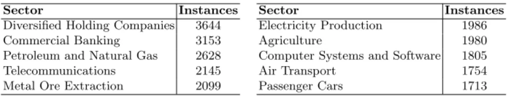
Table 1: Number ofpositiveinstances in the training pool, for the most frequent sectors
Sector Instances Sector Instances
Diversified Holding Companies 3644 Electricity Production 1986
Commercial Banking 3153 Agriculture 1980
Petroleum and Natural Gas 2628 Computer Systems and Software 1805
Telecommunications 2145 Air Transport 1754
Metal Ore Extraction 2099 Passenger Cars 1713
We randomly select up to 600 documents labeled with SN, and split them into
two subsets: 3/4 for the training pool and 1/4 for test. If there are not enough documents (<600) forSN, all available instances are collected, with the same
training/test proportion. In this way we try to guarantee some data will be available for testing, even for the smallest sectors.
We then move on to the second smallest sector,SN−1, and repeat the
collec-tion process, except now we first check how many documents labeled withSN−1
are already present in the training and test pools—which may happen due to
multiple labeling (label overlap). The number of documents collected forSN−1
at this step is reduced by the number already collected. The collection process continues in this manner for all sectors. Collection may be skipped for a sector if it already has more than 450 documents in the training pool (this happens for sectors with high label overlap). As stated, it is also possible that some sectors will have fewer documents for training, based on total availability. These are inherent limitations of the skew in the original corpus, and cannot be avoided.
The resulting set, called the “balanced training data pool” has 77,636 doc-uments. It is still skewed, as seen in Figure 1, on the right, though much more balanced than the initial distribution, shown on the left. As can be inferred from the Figure, between 50 and 60 sectors contain fewer than 150 instances each. Since a lower amount of data makes it difficult to obtain reliable results, we use only the 200 largest sectors in our experiments, which cover approximately 99% of the original corpus.
testing data in random order and happen to start with the largest sectors, then by the time we come to the smallest sectors all of its data may already be included in the training pool (due to multiple labeling of documents), leaving none for testing.
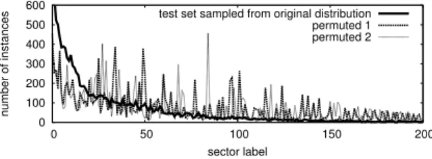
0 100 200 300 400 500 600 0 50 100 150 200 number of instances sector label
test set sampled from original distribution permuted 1 permuted 2
Fig. 2: Label distributions of an original test set, and permuted test-sets (2 of 50 shown).
Table 2: Sector distribution for company “Apple”
Sector Freq Prob
Computer Systems and Software 549 0.61 Electronic Active Components 61 0.07 Datacommunications and Networking 36 0.04
Telecommunications 19 0.02
Electrical and Electronic Engineering 13 0.01
Table 1 shows the most frequent sectors in the balanced training pool. We can see, e.g., that although we only collected 450 positive training instances for
Diversified Holding Companies, it still receives 3644 positive instances in the
pool, most of which were picked up when collecting data for other sectors. For comparison, (Section 7.2), we use anunbalancedtraining pool, which is simply half of the corpus.
All dataoutsidethe balanced and unbalanced training pools—called the “test pool”—are available for the construction of test sets. From the test pool, we generate 10 samples of 10,000 documents each, using the original distribution in the corpus. We use one of these samples as a held-out development set for parameter tuning (Section 4.3), and the remaining nine as test sets.
To simulate the effect of changing trends in news streams, we generate 50 additional datasets. To build these sets, we calculate the individual proportions of the sectors in the original distribution, then assign these proportions to 50
random permutations of the sector labels. We then attempt to sample 10,000
documents from the testing pool according to the new, permuted distributions. Each set among these 50 has its own label distribution, different from both the original and from each other. The distribution of labels in these random test sets will appear “naturally skewed,” since it mimics the original shape.
Three example test sets are shown in Figure 2, one “original,” and two “per-muted.” The permuted distributions are still somewhat biased toward the largest classes in the original corpus. This is expected because some larger classes (such
asDiversified Holding Companies) still have a high degree of overlap, and because
the smallest sectors may not have enough data to dominate the permuted distri-bution. However, the distributions of the permuted test sets look substantially
different from the original distribution and contain significantly more instances from small- and medium-sized sectors. We use the original and permuted test sets in our comparison of balanced and unbalanced training (Section 7.2). 4.3 Classification
The SVM classifiers output a binary decision for every document. For Naive Bayes, the output for each sector is a confidence score between 0.01 and 1; thus a decision threshold is required to make a classification. We learn the best threshold over a range of thresholds (in increments of 0.01), using a held-out
developmentset (one of the test sets, described in Section 4.2). We then evaluate
on the remaining test sets using the learned threshold.
5
Rote classifier
The Rote classifier labels documents based on the company–sector relationships present in the RCV1 corpus. PULS finds mentions of companies in the corpus, using a named-entity (NE) recognition module. It distinguishes company names from other proper names in the text, e.g., persons and locations. NE also merges together variants of the same name, for example, “Apple,” “Apple Inc.,” “Apple Computer, Inc.,” etc. For each company we collect all sector labels from all documents where it is mentioned; sectors co-occurring with a company fewer than 3 times are discarded. For example, Table 2 shows the top sectors that co-occur with “Apple.”; it shows the frequency (the co-occurrence count of the company with the sector), and the proportion, which is the normalized count.
For every document, the Rote classifier returns a sector associated with the companies found in the text if the proportion for this sector is higher than a certain threshold; the threshold is chosen from the range 0.01 to 1, using the development set. If the same sector co-occurs with more than one company found in the text, we apply the highest proportion.
6
Combined Classifiers
We experiment with several methods of combining the Rote classifier, described in Section 5, with the balanced probabilistic classifiers, described in Section 4, to see whether the combination can produce better overall prediction of the sector labels. One method of combining is a simple two-stage process: for each document, we first try to identify sectors using the Rote classifier; if that does not return any sectors, we then attempt to classify using the statistical classifiers. We also experiment with the reverse order of these classification stages. The motivation for this method is to give the overall system a “second chance” at classification, in the hope that together the two methods may overcome their respective shortcomings. Another method of combining classifiers is to return
the union of the results of the two classifiers—rote and probabilistic. Again,
We learn the optimal threshold for each classifier in the combination using the development set.
7
Experiments and Results
7.1 Evaluation MeasuresCommon measures in text classification are precision, recall, and F-measure. For a given classc, these are calculated as:
Recc= T Pc T Pc+F Nc P recc= T Pc T Pc+F Pc F1c= 2×Rec×P rec Rec+P rec
whereT Pc,T Nc,F Pc andF Nc are the number of true positive, true negative,
false positive, and false negative classified instances for the class, respectively;
|c|is the number of documents in the test pool labeled with this class.
In evaluating multi-label classification,macro-averagingandmicro-averaging
are commonly reported, [21]. In micro-average evaluation, first the numbers of true- and false-positives, and true- and false-negatives are counted for all in-stances in the test set, and then the standard measures, e.g., recall or precision, are calculated using these numbers:
Recµ= Σi∈ST Pi Σi∈S(T Pi+F Ni) P recµ= Σi∈ST Pi Σi∈S(T Pi+F Pi) µ-F1 =2×Recµ×P recµ Recµ+P recµ
where S is the set of all classes. In the macro-average evaluation scheme, the measures are calculated for each classseparatelyfirst, and then these are averaged across all classes:
RecM =Σi∈SReci
|S| P recM =
Σi∈SP reci
|S| M-F1 =
Σi∈SF1c |S|
We report both evaluation schemes, although we focus more on the macro-average scores, as explained below, since they are less dependent on the particular distribution of labels in the corpus. Henceforth we denote the macro-averaged F-measure by M-F1, and micro-averaged F-measure byµ-F1.
7.2 Balanced vs. Unbalanced Training
To justify the use of balanced training data in building our classifiers, we com-pare two sets of classifiers, built using two distinct training pools: one balanced, under-sampled training set and one unbalanced training set, comprised of half the total data, selected at random. All data outside these training pools are available for the construction of test sets. As described in Section 4.2, we gen-erate 10 “original” test sets that preserve the original label distribution, and 50 “permuted” test sets with label distributions that are meant to simulate the effect of changing trends in news streams, over time or due to shifts in emphasis toward new sectors in a particular source.
The averaged results obtained on both original and permuted test sets are presented in Table 3. To save space we present only the SVM+IG results, since results for all classifiers follow the same pattern: classifiers trained on the original distribution have higher µ-F1 on originally distributed test sets, but lower on the permuted test sets; the classifiers trained on the balanced training set yield higher M-F1 onall test sets, both original and permuted.
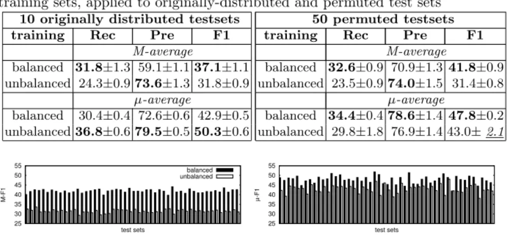
Table 3: Results for SVM+IG classifiers trained on balanced vs. unbalanced training sets, applied to originally-distributed and permuted test sets
10 originally distributed testsets 50 permuted testsets training Rec Pre F1 training Rec Pre F1
M-average M-average balanced 31.8±1.3 59.1±1.137.1±1.1 balanced 32.6±0.9 70.9±1.341.8±0.9 unbalanced 24.3±0.973.6±1.3 31.8±0.9 unbalanced 23.5±0.974.0±1.5 31.4±0.8 µ-average µ-average balanced 30.4±0.4 72.6±0.6 42.9±0.5 balanced 34.4±0.478.6±1.447.8±0.2 unbalanced36.8±0.679.5±0.550.3±0.6 unbalanced 29.8±1.8 76.9±1.4 43.0±2.1 25 30 35 40 45 50 55 M-F1 test sets balanced unbalanced 25 30 35 40 45 50 55 µ -F1 test sets
Fig. 3: F-measure obtained by SVM+IG classifiers trained on balanced vs. un-balanced data, for allpermutedtest sets.
A comparison of balanced and unbalanced training is presented in Figure 3, where we plot macro- and micro-averaged F-measure obtained by classifiers trained on balanced vs. unbalanced data for each permuted test set. As can be seen from the plot in the left figure, the classifier trained on balanced data has significantly and consistently higher M-F1: for each test set M-F1 is over 30% higher for the balanced classifiers.
As seen from the right plot, in the majority of cases, the classifier trained on balanced data also yields higher µ-F1 than the classifier trained on unbal-anced data, although the difference between two classifiers has somewhat higher variance (also seen from Table 3, standard deviation scores). Thus the M-F1 appears to be more stable for both classifiers. This suggests that focusing on macro-averaged results is more appropriate for real-world news classification tasks.
7.3 Comparison of Classifiers and Feature Selection Methods Results obtained by all classifiers are shown in Table 4; we present only results obtained withbalancedtraining data, since they are consistently higher—in terms of M-F1—than results obtained using unbalanced training.
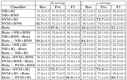
As seen from the table, the SVM classifier yields higher performance than NB, independently of the feature selection method used. IG performs better than BNS with both Naive Bayes and SVM.
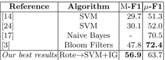
The baseline Rote classifier yields the highest F-measure among single clas-sifiers; combining Rote with SVM+IG yields the best combined performance. The M-F1 obtained by this two-stage classifier is higher than the best previ-ously reported results, as shown in Table 5. It also can be seen from the table
Table 4: Results from all classifiers and feature selection methods, averaged across 9 test sets randomly sampled from original distribution; single classifiers on top, combined classifiers on bottom. For each classifier, the best threshold is trained on one random, originally-distributed development set;→and∪denote, respectively, two-stage and union combining methods, described in Section 6.
M-average µ-average
Classifier Rec Pre F1 Rec Pre F1
NB+IG 31.3±0.9 21.9±0.6 19.7±0.6 31.5±0.5 22.4±0.6 26.2±0.5 NB+BNS 34.2±1.1 16.6±0.6 15.8±0.5 33.1±0.7 13.4±0.4 19.0±0.5 SVM+IG 31.9±1.3 59.2±1.1 37.1±1.2 30.5±0.472.7±0.6 42.9±0.4 SVM+BNS 32.7±0.9 55.2±1.0 36.2±0.7 30.1±0.5 70.8±0.6 42.2±0.5 Rote 35.0±0.867.6±1.0 43.8±0.8 42.4±0.6 64.2±0.451.1±0.5 Rote→NB+BNS 51.5±0.9 33.6±0.4 36.1±0.4 57.6±0.6 39.1±0.4 46.6±0.4 NB+BNS→Rote 49.7±1.0 24.0±0.2 26.9±0.3 53.3±0.4 23.7±0.3 32.8±0.3 Rote∪ NB+BNS 59.2±0.9 25.4±0.3 30.7±0.3 64.3±0.5 26.2±0.3 37.2±0.3 Rote→NB+IG 51.8±0.9 39.8±0.6 41.5±0.6 59.1±0.5 47.3±0.4 52.5±0.4 NB+IG→Rote 48.7±1.0 31.5±0.5 33.4±0.4 53.0±0.5 36.3±0.3 43.1±0.3 Rote∪ NB+IG 57.2±0.9 32.7±0.4 37.3±0.4 63.2±0.5 38.1±0.3 47.5±0.4 Rote→SVM+BNS 48.2±1.0 67.5±1.0 54.7±0.9 53.7±0.5 70.1±0.3 60.8±0.4 SVM+BNS→Rote 48.0±1.1 63.0±1.0 52.6±1.0 50.2±0.4 70.8±0.4 58.7±0.4 Rote∪ SVM+BNS 54.0±0.9 62.0±0.8 56.1±0.8 58.5±0.4 68.2±0.3 63.0±0.3 Rote→SVM+IG 46.2±1.073.7±0.8 55.1±0.8 52.5±0.575.9±0.4 62.0±0.4 SVM+IG→Rote 47.0±1.2 67.7±0.9 53.7±1.1 49.9±0.3 73.9±0.3 59.6±0.3 Rote∪ SVM+IG 52.2±1.1 66.3±0.856.9±0.9 57.7±0.4 71.1±0.363.7±0.4
that the difference between M-F1 and µ-F1 for our classifiers is smaller than that reported in prior work. This supports the claim that our classifiers are less sensitive to changes in label distribution (due to the balancing of the training), which is one of our main objectives.
The µ-F1 in our experiments is lower than the best µ-F1 reported in the literature on RCV1. This is likely due to the fact that both [17] and [3] try to model inter-dependencies among the labels in the corpus. This is not done in [14] or [24]. We plan to investigate this further in future work; however, our results suggest that balancing the training data improves the classifier performance overall, regardless of the method used.
8
Conclusion
We have described an approach using supervised learning for labeling business-news documents with multiple industry sectors. We treat the class, multi-label problem as a set of binary sub-tasks, with one binary classifier for each sec-tor. We attempt to create robust classifiers, suitable for real-world text classifica-tion (rather than improving performance on a given static corpus), by balancing
Table 5: Classification results on RCV1 industry sectors, compared with state of the art. Reference Algorithm M-F1µ-F1 [14] SVM 29.7 51.3 [24] SVM 30.1 52.0 [17] Naive Bayes - 70.5 [3] Bloom Filters 47.8 72.4 Our best resultsRote→SVM+IG 56.9 63.7
the training data given to each classifier. Our results suggest that, compared to classifiers trained on labels drawn from the original corpus distribution, the bal-anced training helps improve the scores—M-F1 in particular—when classifying data drawn from different distributions of labels.
We explore several combinations of learning algorithms and feature selection methods, and evaluate them using a large number of manually-labeled docu-ments. Combining a named-entity-based Rote classifier with the set of balanced classifiers, into a two-stage classifier, yields better results than either classifier alone. Additionally, this method improves on the best M-F1 previously reported, while using the same amount of training data for the Rote classifier, and con-siderably less for the statistical classifiers.
References
1. Boutell, M.R., Luo, J., Shen, X., Brown, C.M.: Learning multi-label scene classifi-cation. Pattern Recognition 37(9) (2004)
2. Chawla, N.V., Bowyer, K.W., Hall, L.O., Kegelmeyer, W.P.: Smote: Synthetic minority over-sampling technique. Journal of Artificial Intelligence Research 16(1), 321–357 (2002)
3. Cisse, M.M., Usunier, N., Arti, T., Gallinari, P.: Robust Bloom filters for large mul-tilabel classification tasks. In: Advances in Neural Information Processing Systems. pp. 1851–1859 (2013)
4. Dendamrongvit, S., Kubat, M.: Undersampling approach for imbalanced training sets and induction from multi-label text-categorization domains. In: New Frontiers in Applied Data Mining, pp. 40–52. Springer (2010)
5. Dhondt, E., Verberne, S., Weber, N., Koster, C., Boves, L.: Using skipgrams and pos-based feature selection for patent classification. Computational Linguistics in the Netherlands (2012)
6. Erenel, Z., Altın¸cay, H.: Improving the precision-recall trade-off in undersampling-based binary text categorization using unanimity rule. Neural Computing and Applications 22(1), 83–100 (2013)
7. Forman, G.: An extensive empirical study of feature selection metrics for text classification. Journal of Machine Learning Research 3, 1289–1305 (Mar 2003) 8. Hall, M., Frank, E., Holmes, G., Pfahringer, B., Reutemann, P., Witten, I.H.: The
WEKA data mining software: an update. ACM SIGKDD Explorations Newsletter 11(1), 10–18 (2009)
9. Huang, R., Riloff, E.: Classifying message board posts with an extracted lexicon of patient attributes. In: Proceedings of the 2013 Conference on Empirical Methods in Natural Language Processing. pp. 1557–1562 (2013)
10. Huttunen, S., Vihavainen, A., Du, M., Yangarber, R.: Predicting relevance of event extraction for the end user. In: Poibeau, T., Saggion, H., Piskorski, J., Yangarber, R. (eds.) Multi-source, Multilingual Information Extraction and Summarization, pp. 163–176. Theory and Applications of Natural Language Processing, Springer Berlin (2012)
11. Japkowicz, N., Stephen, S.: The class imbalance problem: A systematic study. Intelligent data analysis 6(5), 429–449 (2002)
12. Koller, D., Sahami, M.: Hierarchically classifying documents using very few words. Technical Report 1997–75, Stanford InfoLab (February 1997)
13. Kotsiantis, S., Kanellopoulos, D., Pintelas, P., et al.: Handling imbalanced datasets: A review. GESTS International Transactions on Computer Science and Engineer-ing 30(1), 25–36 (2006)
14. Lewis, D.D., Yang, Y., Rose, T.G., Li, F.: RCV1: A new benchmark collection for text categorization research. The Journal of Machine Learning Research 5, 361–397 (2004)
15. Liu, Y., Loh, H.T., Sun, A.: Imbalanced text classification: a term weighting ap-proach. Expert Systems with Applications 36(1), 690–701 (2009)
16. Prati, R.C., Batista, G.E., Monard, M.C.: Class imbalances versus class overlap-ping: An analysis of a learning system behavior. In: MICAI 2004: Advances in Artificial Intelligence: Third Mexican International Conference on Artificial Intel-ligence, Mexico City, Mexico, April 26-30, 2004, Proceedings. vol. 3, pp. 312–321. Springer (2004)
17. Puurula, A.: Scalable text classification with sparse generative modeling. In: An-thony, P., Ishizuka, M., Lukose, D. (eds.) PRICAI 2012: Trends in Artificial Intelli-gence, Lecture Notes in Computer Science, vol. 7458, pp. 458–469. Springer Berlin Heidelberg (2012)
18. Stamatatos, E.: Author identification: Using text sampling to handle the class imbalance problem. Information Processing & Management 44(2), 790–799 (2008) 19. Tikk, D., Bir´o, G.: Experiments with multi-label text classifier on the Reuters collection. In: Proceedings of the International Conference on Computational Cy-bernetics (ICCC 03). pp. 33–38 (2003)
20. Tsoumakas, G., Katakis, I.: Multi-label classification: an overview. International Journal of Data Warehousing and Mining (IJDWM) 3(3), 1–13 (2007)
21. Yang, Y.: An evaluation of statistical approaches to text categorization. Informa-tion retrieval 1(1-2), 69–90 (1999)
22. Yang, Y., Pedersen, J.O.: A comparative study on feature selection in text catego-rization. In: ICML. vol. 97, pp. 412–420 (1997)
23. Zhang, W., Yoshida, T., Tang, X.: A comparative study of TF*IDF, LSI and multi-words for text classification. Expert Systems with Applications 38(3), 2758 – 2765 (2011)
24. Zhuang, D., Zhang, B., Yang, Q., Yan, J., Chen, Z., Chen, Y.: Efficient text clas-sification by weighted proximal SVM. In: Fifth IEEE International Conference on Data Mining (2005)