\
Sermpinis, G. , Tsoukas, S. and Zhang, P. (2018) Modelling market implied
ratings using LASSO variable selection techniques.
Journal of Empirical
Finance
, 48, pp. 19-35. (doi:
10.1016/j.jempfin.2018.05.001
)
There may be differences between this version and the published version.
You are advised to consult the publisher’s version if you wish to cite from
it.
http://eprints.gla.ac.uk/164498/
Deposited on 25 June 2018
Enlighten – Research publications by members of the University of
Glasgow
Modelling market implied ratings using LASSO variable selection
techniques
1by
George Sermpinis, Serafeim Tsoukas, Ping Zhang University of Glasgow
January 2018
Abstract
Making accurate predictions of corporate credit ratings is a crucial issue to both investors and rating agencies. In this paper, we investigate the determinants of market implied credit ratings in relation to financial factors, market-driven indicators and macroeconomic predictors. Applying a variable selection technique, the least absolute shrinkage and selection operator (LASSO), we document substantial predictive ability. In addition, when we compare our LASSO-selected models with the benchmark ordered probit model, we find that the former models have superior predictive power and outperform the latter model in all out-of-sample predictions.
Key words: Market implied ratings, LASSO, Financial ratios, Forecasting
JEL: G24, G33, C25, O16
1 We are grateful for comments and inputs from an anonymous referee, Oldrich Vasicek and from participants
at the 2017 European Financial Management Association Conference, the 2017 European Meetings of the Econometric Society, the 2016 International Conference on Forecasting Financial Markets and the Adam Smith Business School seminars. Corresponding Author: Serafeim Tsoukas, email: [email protected]. Adam Smith Business School, University of Glasgow, G12 8QQ, Tel: +44 141 3306325. The third author is grateful to China Scholarship Council for funding (Grant number: 201508060273). Any remaining errors are our own.
2
1.
Introduction
Recent turmoil in the financial markets has focused attention on the rating agencies and the process by which they assign ratings to firms and their financial obligations. A careful management of credit risk is high the agenda for both market participants and regulators. It is well known that the credit ratings of the top three nationally recognized statistical rating organizations (NRSROs), Standard and Poor’s, Moody’s and Fitch play a key role in the pricing of credit risk and in the delineation of investment strategies since they measure the firm’s long-term ability and willingness to meet debt servicing obligations. As such, the ratings indicate the probability that a given borrower will default. However, the accuracy and the timing of the ratings have been heavily criticized, especially during the most recent financial crisis. It has been argued that the standard agency ratings do not adjust quickly to price changes and therefore may be out of date. In response to these concerns, Fitch has recently developed a new model to derive Market Implied Ratings (MIRs) from bond and equity prices. The obvious advantage of these ratings compared to the conventional agency ratings is that they adjust instantaneously to price changes.
This study offers methodological extensions applying a variable selection approach, the least absolute shrinkage and selection operator (LASSO), and its most promising derivation, the Elastic net, into ordered probit and continuation ratio models, to the task of predicting Fitch’s CDS and Equity implied ratings (CDSIRs and EQIRs respectively hereafter). The research aims to exploit the LASSO properties and unveil the underlying structure of CDSIRs and EQIRs.2
There are several studies that use accounting ratios and other publicly available information in reduced-form models in order to predict credit ratings. These studies use various techniques (OLS, multinomial and ordered logit/probit models) to identify the most important characteristics for predicting bond ratings (see for instance the early studies by Poldue and Soldofsky, 1969, Pinches and Mingo, 1973, Kaplan and Urwitz, 1979 and Kao and Wu, 1990). The upshot is that financial healthiness is associated with ratings determination and prediction of default. Another line of research advocates the importance of estimating the
2 With respect to the latter aim of this study, we do not report estimated coefficients of the prediction models
models in a dynamic setting and documents a noticeable improvement in the predictive ability of the models once state dependence is controlled for (see Mizen and Tsoukas, 2012). One drawback of the reduced-form models, discussed above, is that they tend to employ many rating predictors as inputs despite the fact that only a sub-set is relevant. This has two critical implications. First, this approach can omit potentially important determinants leading to a decrease in prediction accuracy. Second, given the large number of predictors included, it does not provide a sparse representation, implying that these models cannot be readily used by market participants and rating agencies.
Our approach is mostly related to the literature that examines the determinants of credit ratings, but we add to it in two important ways. First, we make a methodological contribution by deriving a simple and more intuitive, yet innovative model, which is based on the variable selection technique, pioneered the by Tibshirani (1996)—the least absolute shrinkage and selection operator (LASSO). It is well accepted that this selection approach not only helps in identifying the most relevant predictors from an extensive set of candidate variables, but also improves the predictive power (see Fan and Li, 2001 and Tian et al, 2015). In addition, LASSO does not require strict assumptions such as a pre-selection of the variables considered and it is consistent statistically as the number of observations approach infinity (Van de Geer, 2008). Importantly, LASSO can potentially sidestep the problem of multicollinearity, which is fairly common in probit/logit models, and it is computationally efficient even when considering a large set of potential predictors. Our study is the first, as far as we know, to provide a systematic empirical analysis of LASSO in MIRs forecasts. In doing so, we explore the relative importance of several time-varying covariates from an extensive set of firm-, market-specific and macro-economic explicators used to predict market implied ratings. This is important as we provide a parsimonious set of predictors that can be readily implemented by investors, managers and credit risk agencies.
Second, we use a data-set made up by MIRs instead of the standard long-term ratings. The former type of ratings represents an innovation to the ratings industry to address the issue of staleness in their long-term counterparts. The market implied ratings rely on proprietary and data-intensive rating models that incorporate market information into a model-based credit
4 assessment (see for instance, Rösch, 2005 and Tsoukas and Spaliara, 2014). The most appealing characteristic of these ratings is that they can adjust instantly to market changes. Hence, we build on the foundations of the literature on implied (or point-in-time ratings) by investigating the forecasting power of models that capture volatile market changes.
To preview our findings, we show that several financial factors along with market-driven and macroeconomic variables contain information about market implied ratings. Importantly, when applying the LASSO techniques, we are able to significantly improve the predictive power of our models in out-of-sample predictions compared to the ordered probit model, which is commonly adopted in the literature. Moreover, we note that the LASSO models with BIC-type tuning parameter selector outperform their LASSO counterparts with AIC-type selector for the dataset and periods under study. Thus, LASSO-selected models display improved forecasting power.
The rest of the paper is laid out as follows. In section 2 we discuss the relevant literature. Section 3 presents the data and summary statistics. In section 4 we describe our methodology. In Section 5 we report the empirical results and robustness tests. Section 6 concludes the paper.
2.
Related literature
The issue of how rating agencies use public information in setting quality ratings has attracted considerable attention in the literature. In fact, the literature goes as far back as Horrigan (1966). This study presents the first attempt to predict ratings based on the characteristics of the bonds and the issuing firms. The author concentrates on accounting data and financial ratios in order to find the most appropriate predictors. The set of preferred variables contains total assets, net worth to total debt, net operating profit to sales and working capital. Poldue and Soldofsky (1969) also assign ordinal numbers to ratings and investigate different accounting variables as potential determinants. They conclude that the most significant independent variables are long-term debt to total assets, the coefficient of variation of
earnings, and total assets.3 West (1970) challenge Horrigan’s study by using another set of
explanatory variables namely earnings volatility, capital structure, reliability and marketability. Based on values of the obtained R-squared, the author claims that the proposed model has a better explanatory power.
Pinches and Mingo (1973) adopt a two-stage approach to assign ratings to bond issues. This study attempts to test the predicting ability of a small number of explanatory variables using multiple regression and discriminant analysis. The proportion of correct predictions lie in the region of 70 percent. Moreover, Kaplan and Urwitz (1979) confirm the above studies by using an ordered probit analysis. They show that ratings may be reasonably well predicted using balance sheet information. Other studies that use a small number of explanatory variables (e.g leverage, profitability, interest coverage, firm’s size and subordination status) to predict credit ratings include Ederigton (1985) and Gentry et al (1988). The former study uses long-term debt, subordination, total assets and interest coverage as explanatory variables, while the later focuses on subordination, size of issue, debt ratio, cumulative years that dividends were paid and net income to interest.
Blume et al. (1998) depart from the traditional examination of credit ratings determinants by considering whether there is any tendency for a company that maintains the same values of accounting ratios over time to receive a lower rating due to worsening of rating standards. Using an ordered probit analysis they find that rating agencies have changed the way in which they evaluate credit standing and they report a secular tightening of rating agency standards. They conclude that it became more difficult for firms to obtain improved ratings in the mid-1980s and early 1990s.
More recently, ordered probit methodologies are employed by Hwang et al., (2009) and Hwang et al., (2010) to forecast credit ratings. Both studies show that several predictors are important in forecasting credit ratings such as the size of the company, balance sheet position, stock market performance and industry effects. In addition, modelling long-term ratings in a dynamic setting has shown improvements in forecasting (see Hwang, 2011 and Hwang, 2013).
6 In a similar vein, Mizen and Tsoukas (2012) find that allowing for persistence in ratings significantly improves the forecasting power of long-term ratings. In a subsequent study, Tsoukas and Spaliara (2014) use the market implied ratings and the ordered probit modelling strategy to investigate the role of financial constraints. They conclude that financial variables are more important in predicting credit ratings for firms likely to face financing constraints.
The literature on market implied ratings has focused on the comparison between long-term agency ratings and market implied ratings. Breger et al. (2003) use bond spreads to find suitable thresholds categorizing bonds. They find that implied ratings are a superior application to identify default probability in the rating system. Rösch (2005) documents that implied ratings can provide more accurate default probability forecasts than long-term ratings. Castellano and Giacometti (2012) note that MIRs can be regarded as early warning signals of credit rating changes.
Moving to the line of work on variable selection techniques, there is only a handful of papers investigating default probabilities in various settings. Härdle and Prastyo (2013) employ the LASSO approach to predict default probability in a sub-set of Asian economies. Amendola et al, (2012) evaluate the default risk in the limited liability sector in Italy. Finally, Tian et al., (2015) evaluate the probability of bankruptcy using a comprehensive sample of US firms. The authors conclude that the accuracy in the out-of-sample prediction can be superior to previous studies of estimating default by combining reduced-form models with the LASSO procedure.
The studies discussed above provide a useful background on the credit ratings procedure and the selection process of relevant predictors. In the sections that follow we turn to our data and estimation strategy.
3.
Data and summary statistics
3.1Data sourcesThe data on market implied ratings are taken from Fitch’s database and refer to solicited ratings for all traded US corporations. This database provides information on the CDS and
Equity implied ratings assigned to each issuer as well as the date that the rating became available. Both CDS and Equity implied ratings are reported on a monthly frequency and span the period 2002 to 2008.4 In keeping with the normal practice in the literature, we categorize
our firms into rating buckets without consideration of notches (i.e + or -). Amato and Furfine (2004) and Mizen and Tsoukas (2012) note that this classification takes into account large cumulative changes of ratings rather than small movements notch by notch, and avoids generation of rating categories with very few observations.Therefore, we consider seven rating categories, ranging from AAA to Below CCC, which are assigned numerical values in Table 1, starting with 1 to AAA, 2 to AA…, 7 to Below CCC.5
Insert Table 1
Firm-specific accounting data are extracted from Fitch’s Peer Analysis Tool. Corporate historical data for all firms rated by Fitch are available on a quarterly basis from this database. For these firms with credit ratings, we link their ratings to Fitch’s balance sheet statements and profit and loss accounts. Hence, our dataset is constructed by merging monthly market implied ratings data and quarterly firm-level accounting data. 6 In other words, we have an
entry for each firm-month with CDSIRs and EQIRs data and financial and market data. Following commonly used selection criteria in the literature; we exclude companies that do not have complete records on our explanatory variables and firm-months with negative sales and assets. To control for the potential influence of outliers, we winsorize the regression variables at the 1st and 99th percentiles.
Data on market indicators and macroeconomic variables are sourced from Bloomberg. These data items are reported monthly. Our combined sample contains data for 211 firms that
4 The research aims to study the structure and the predictability of the implied ratings in the years preceding the
recent global financial crisis. Our choice to focus on a time window ending in 2008 is motivated by two important considerations. First, the global financial crisis and the collapse of Lehman Brothers constitute a shock that may have acted as a confounding factor to the determination of credit ratings. In fact, it can be argued that the misinterpretation of the credit ratings by investors was one of the main contributors to the crisis. Second, the data were downloaded early in 2010 owning to a research project supported by Fitch: the coverage period is therefore 2002-2008.
5 In EQIRs we do not observe any ratings in the last category, hence six groups are generated for this type of
implied ratings.
6 For each firm, the quarterly data is repeated every month during the same quarter if the monthly data is not
8 operate in all sectors of the US economy except agriculture, forestry and fishing and public administration. The panel has an unbalanced structure with the number of observations on each firm varying between 1 and 63. Our sample presents two characteristics that make it especially appealing for our analysis. First, it includes both investment and speculative grades ratings in line with previous studies (see for instance Amato and Furfine, 2004). This is particularly beneficial since we can cover the entire spectrum of firms. Second, the distribution of agency (long-term) ratings in CDS data is very similar to the distribution of agency ratings in the general bond population (see Fitch 2007). Thus, both the CDSIRs and the EQIRs databases can provide a representative base for conducting our empirical analysis. 3.2Choice of explanatory variables
Prior empirical research on the determinants of credit ratings has considered both business and financial risks. The former type of risk includes an assessment of industry characteristics, firm size, management capability and organizational factors. The latter concerns the quality of a firm’s accounting procedures, profitability, cash flow situation and its overall financial policy. In the market implied ratings, models typically consider market-related information in addition to the above-mentioned factors. With that in our mind, we also turn to rating agencies and in particular to Fitch, to find out what matters when assigning a market implied rating. In other words, the selection of our explanatory variables is guided both from the existing empirical literature (see for example Kaplan and Urwitz, 1979; Ederington, 1985; Poon, 2003; Chava and Jarrow, 2004; Amendola et al, 2011; Mizen and Tsoukas, 2012; Hwang, 2013; Creal et al, 2014; Doumpos et al, 2015 and Tian et al, 2015), and the common practice of rating agencies (see Fitch 2007 and Liu et al. 2007).7
3.2.1 Firm-specific variables
We consider 16 firm-specific accounting variables as potential predictors of ratings. These variables are intended to measure different aspects of firms’ financial health, these are size, leverage, coverage, cash flow, profitability and liquidity. Specifically, we employ the firm size
7 The expected relationship between these variables and MIRs is presented in Table A1 in on-line Appendix A.
(DETA) as measured by the natural logarithm of firms’ real total assets. Size accounts for the scale of the firm and would be expected to improve the rating. Next, we proxy leverage using a number of ratios: The ratio of long-term debt to total assets (LDA), the ratio of short-term debt to total assets (SDA), the ratio of total debt over total assets (TDA), the ratio of total assets over equity (AE), and the ratio of total debt to earnings before interest, taxes, depreciation, amortization, and restructuring or rent costs (TDEBITDA). Higher values of the above ratios are likely to increase financial risk and hence should worsen the rating. The next two measures capture the creditworthiness of the firm as they show the firm’s ability to generate income to meet interest rate obligations: the ratio of earnings before interest and tax over interest expenses (EBITINT) and the ratio of total debt to earnings before interest, taxes, depreciation, amortization, and restructuring or rent costs to interest expenses (EBITDAINT). Both ratios would improve the credit rating if they were to increase. Further, cash flow is measured by the following ratios: cash flow from operating activities over total assets (CFOA), and cash and equivalent over total assets (CASHEQA). We expect firms with higher cash flows to have improved ratings. The following five ratios measure firm profitability: The ratio of operating income to net sales (OM), the ratio of net income without dividends over total capital (ROC), the ratio of net income over shareholders’ equity (ROE), the ratio of net income over total assets (ROA) and the ratio of the funds from operations to total debt (FFD). An increase in the above-mentioned profitability ratios should be associated with an improvement of ratings. Finally, liquidity is measured by the ratio of cash from operations to liabilities (LIQ), which indicates a firm’s ability to satisfy its short-term obligations as they become due. Higher levels of liquidity should improve credit ratings.
3.2.2 Market-driven indicators
As noted above, market implied ratings are likely to be determined by market-related conditions. Therefore, we employ the following market indicators: Excess return (EXRET) as measured by the monthly stock return on the firm minus the S&P 500 index return. The relative size of a firm in market (RSIZE) measured by each firm’s market equity value divided by the total market equity value. The above-mentioned variables should be positively correlated with ratings upgrades. Next, we use the volatility of stock return (STD) which is calculated as the standard deviation of each company’s monthly stock returns. We also use
10 the systematic risk of each firm (BETA), measured by the Capital Asset Pricing Model for each firm. Finally, we extract the 1-year and 5-year default probabilities (PD1 and PD5) from the Fitch’s Peer Analysis Tool. All three variables should worsen ratings if they were to increase.
3.2.3 Macroeconomic influences
We also consider an extensive list of macro-economic covariates as potential predictors of market implied ratings. Specifically, the stock market performance is evaluated by the S&P 500 return, which calculates returns on the S&P 500 index (RLSP). The short-term interest rate as measured by the three-month commercial paper rate (CPFFM), three-month Treasury bill rate minus federal funds rate (TB3) and the one-year constant maturity treasury rate (GS1). We also employ the general price level, as measured by the growth rate in the narrow money stock (MB) and inflation rate (INFL). The aggregate economic activity is captured by the rate of change in industrial production (DLIP), the index of the growth rate of real GDP (DLGDP), the average of monthly Chicago Fed National Activity Index over the year (CFNA), the average of monthly unemployment rate over the year (UNRATE) and the Chicago Board Options Exchange (CBOE) volatility index (VIX). All macro-variables, apart from VIX, are reported in percentages. The eleven macroeconomic variables measure different aspects of the aggregate economy’s performance. Their relationship with the market implied ratings could be either positive or negative as ratings tend to improve during good times but agencies have been observed to tighten their standards during these periods. Hence, the relationship between ratings and macro-economic variables is an issue that will be determined empirically.
3.3Summary statistics
Tables 2 and 3 illustrate the distribution of firms by rating category for CDSIRs and EQIRs, respectively. It can be observed that the distribution of firms across the rating categories is quite stable and that most companies are assigned A and BBB ratings.
Insert Table 2 Insert Table 3
At the next stage, we report summary statistics for our explanatory variables in Tables 4 and 5. We present statistics splitting the sample between investment grade and non-investment grade to gauge any differences across ratings categories. P-values for the tests of equality of means across the above-mentioned groups are reported in the last columns of the tables. We observe, as expected, that firms in the investment grade group display better financial characteristics, as measured by the balance sheet indicators. The tests point to significant differences between the two groups, which indicate that there is a correlation between better financial health and an improved rating. In other words, there is considerable cross-sectional variation in market implied ratings. Moving to the market indicators, we find that improved market conditions are associated with investment grade ratings, which also suggests a link between the market climate and the ratings.
Insert Table 4 Insert Table 5
4. Methodology
We predict the changes in market implied ratings with ordered probit (OP) and continuation ratio (CR) models combined with LASSO or the Elastic net. The proposed methodology aims at selecting the most important predictors and at providing accurate MIRs forecasts. LASSO, originally proposed by Tibshirani (1996), is an extended form of an OLS regression which performs both variable selection and regularization through a shrinkage factor. It is capable of enhancing the accuracy and the interpretability of classical regression methods (Tibshirani, 1996). To maintain the properties of LASSO and capture the ordinal ranking of MIRs, penalty functions from LASSO or its variant (Elastic net) are added into OP or CR models. This helps us unveil the relation between the potential predictors (at the firm and macro level) and identify their significance in predicting MIRs. As benchmark to our study, we rely to the standard OP model. A description of the empirical modelling strategy follows.
4.1OP
MIRs as a branch of credit ratings are discrete-valued signs and have an ordinal ranking. To meet the ordinal property of MIRs, OP is applied naturally as a benchmark in the relevant literature (Kaplan and Urwitz, 1979; Gentry, 1988; Blume et al., 1998; Amato and Furfine,
12 2004 and Hwang et. al., 2009). OP takes into account both the existence of ordinal ranking and the difference between any two adjacent ratings8. We define the categorical variable
𝑦𝑖𝑡 = 1, 2. . . , 7 according to the rating assigned to each firm. We assume that there is an unobservable dependent variable 𝑦𝑖𝑡∗associated with 𝑦𝑖𝑡, which can be expressed as:
𝑦𝑖𝑡∗ = 𝑋𝑖𝑡𝛽1+ 𝑋𝑖𝑡−1𝛽2+ 𝑋𝑖𝑡−2𝛽3+ 𝑋𝑖𝑡−3𝛽4+ 𝑊𝑖𝑡𝛽5+ 𝑊𝑖𝑡−1𝛽6+ 𝑊𝑖𝑡−2𝛽7+ 𝑊𝑖𝑡−3𝛽8+
𝑍𝑖𝑡𝛽9+ 𝑍𝑖𝑡−1𝛽10+ 𝑍𝑖𝑡−2𝛽11+ 𝑍𝑖𝑡−3𝛽12+ 𝑦𝑖𝑡−1𝛽13+ 𝜀𝑖𝑡, (1) where 𝑖 = 1, 2, … , 𝑁 represents firms, and 𝑡 = 1, 2, … , 𝑇 represents different time periods. In this context, 𝑡 is the month end for monthly data. 𝛽 are vectors of unknown parameters to be estimated. 𝑋 denotes a set containing 16 accounting variables, which can be divided into broad groups of size, leverage, coverage, cash flow, profitability and liquidity. 𝑊and 𝑍 contain 6 market-driven variables and 11 macroeconomic variables, respectively. Following the literature (Güttler and Wahrenburg, 2007), all predictors in 𝑋, 𝑊 and 𝑍 are lagged three periods denoted by 𝑡 − 1, 𝑡 − 2 𝑎𝑛𝑑 𝑡 − 3 to mitigate potential time tendency. To capture potential non-linear influences, we allow for non-linear transformation of the variables and therefore the square of each predictor is considered and included9. Thus, the total number of
firm-specific accounting, market driven and macroeconomic variables is 26410. 𝑦
𝑖𝑡−1 is an indicator of the firm’s rating in the previous time periods. We consider 4 lags to control for state dependence. The concern of persistency in ratings is an important dimension of time-series variation and the use of models with lagged rating categories is the standard way of addressing this issue11. The error term 𝜀
𝑖𝑡 in equation (1) is assumed to be a normally
8 For details on the exposition of the OP, see Maddala (2008, pp 47-48).
9 This approach is justified theoretically since some variables may have a positive effect up to a certain (turning)
point and negative thereafter.
10 We consider 16 accounting variables, 6 market-driven variables, 11 macroeconomic variables and their first
three lags (in total, 132 variables). We also consider the square of these variables, thus in equation (1) we have in total 268 variables made up by 264 firm-specific accounting, market driven and macroeconomic variables and 4 state dependence variables. We use the same set of predictors throughout the paper.
11 State dependence captures previous rating state and indicates the realization of a rating in the previous time
period. Following Contoyannis et. al. (2004) and Mizen and Tsoukas (2012), the state dependence is controlled for by applying dummy variables representing first lags of each category in the dependent variable. Given that we observe limited observations in the extreme high and low rating categories, these ratings in the state dependence variables are merged into 5 groups, such as above AA ratings, A rating, BBB rating, BB rating and below B ratings. In addition, to avoid the dummy variable trap we omit one baseline rating category. Therefore, the lagged rating category BBB is not included in the models because it is regarded as the baseline category of lagged MIRs.
distributed residual with a zero mean and unit variance. In our data 𝑦𝑖𝑡∗ is not observed. Thus what is observed are the market implied ratings assigned to firms, which can take M values. The relation between the observed variable 𝑦𝑖𝑡 and the latent variable 𝑦𝑖𝑡∗ it is assumed to be given by:
𝑦𝑖𝑡= 𝑚 𝑖𝑓 𝛼𝑚−1< 𝑦𝑖𝑡∗ ≤ 𝛼𝑚 𝑓𝑜𝑟 𝑚 = 1, … , 𝑀 (2) For a set of parameters 𝛼0 to 𝛼𝑀, where 𝛼0<𝛼1<…<𝛼𝑀, 𝛼0= −∞ and 𝛼𝑀= ∞. Assuming a standard normal distribution for 𝜀𝑖𝑡, the conditional probabilities can be derived as:
𝑃𝑟(𝑦𝑖𝑡= 𝑚) =Φ(𝛼𝑚− 𝑋𝑖𝑡𝛽1− 𝑋𝑖𝑡−1𝛽2− 𝑋𝑖𝑡−2𝛽3− 𝑋𝑖𝑡−3𝛽4− 𝑊𝑖𝑡𝛽5− 𝑊𝑖𝑡−1𝛽6−
𝑊𝑖𝑡−2𝛽7− 𝑊𝑖𝑡−3𝛽8− 𝑍𝑖𝑡𝛽9− 𝑍𝑖𝑡−1𝛽10− 𝑍𝑖𝑡−2𝛽11− 𝑍𝑖𝑡−3𝛽12− 𝑦𝑖𝑡−1𝛽13) −Φ(𝛼𝑚−1−
𝑋𝑖𝑡𝛽1− 𝑋𝑖𝑡−1𝛽2− 𝑋𝑖𝑡−2𝛽3− 𝑋𝑖𝑡−3𝛽4− 𝑊𝑖𝑡𝛽5− 𝑊𝑖𝑡−1𝛽6− 𝑊𝑖𝑡−2𝛽7− 𝑊𝑖𝑡−3𝛽8− 𝑍𝑖𝑡𝛽9−
𝑍𝑖𝑡−1𝛽10− 𝑍𝑖𝑡−2𝛽11− 𝑍𝑖𝑡−3𝛽12− 𝑦𝑖𝑡−1𝛽13), (3) Where Φ(.) is the standard normal distribution function. We can evaluate the above probabilities for any combination of parameters in the vectors 𝛼 and 𝛽.
4.2OP with LASSO
According to Tibshirani (1996), LASSO is a method of regression that enables estimation and variable selection simultaneously in a non-orthogonal setting. Under a suitable choice of penalty power, LASSO selects variables by forcing some coefficients to zero and shrinking others. This reduces the variance of the estimated value and increases the accuracy of the regression prediction. The LASSO estimator resolves the 𝑙1-penalized OP problem of estimating 𝛽 by maximizing a likelihood function. In particular, the maximization of the likelihood proceeds subject to the constraint ∑𝑝𝑞=1|𝛽𝑞|≤ 𝑠, where 𝑠 is a user-specified tuning parameter and 𝑞 = 1, 2. . . 𝑝 indicates the number of surviving predictors with non-zero estimated coefficients. This penalty corresponds to the L1 norm, and therefore it is often referred to as L1 penalized model. The OP with LASSO (L1 penalized OP model) can then be expressed as:
14 𝛽̂ = 𝑎𝑟𝑔𝑚𝑎𝑥𝛽(ℓ(𝛽|𝑦𝑖𝑡, 𝛢) − 𝜆 ∑|𝛽𝑞| 𝑝 𝑞=1 ), (4)
where ℓ(𝛽|𝑦𝑖𝑡, 𝛢) is the likelihood function of OP and 𝛢 contains the pool of the potential predictors (𝑋𝑖𝑡, 𝑋𝑖𝑡−1, 𝑋𝑖𝑡−2, 𝑋𝑖𝑡−3, 𝑊𝑖𝑡, 𝑊𝑖𝑡−1, 𝑊𝑖𝑡−2, 𝑊𝑖𝑡−3, 𝑍𝑖𝑡, 𝑍𝑖𝑡−1, 𝑍𝑖𝑡−2, 𝑍𝑖𝑡−3, 𝑦𝑖𝑡−1). All explanatory variables are standardized before applying the LASSO estimator. In equation (4), λ stands for the tuning parameter. As λ increases the sum of absolute values of estimated coefficients is reduced and shrinkage of coefficients is achieved. If λ exceeds a threshold value in the corresponding models, some estimated coefficients are set to zero ultimately. This ‘‘L1 norm penalty’’ or the constraint formulation in LASSO generates a more interpretable and sparse model.
As already noted, compared with other independent variable selection methods, LASSO can provide more stable and restricted models (Tibshirani, 1996; Fan and Li, 2001; Zou, 2006 and Tian et.al., 2015). It is also a computationally simple and efficient method (Efron et al., 2004). Several approaches, such as cross validation and information criteria, have been proposed in selecting latent models with minimum prediction errors or maximum log-likelihood estimation. Zou et.al. (2007) provide an efficient approach to obtain the optimal LASSO fit with the Akaike information criterion (AIC) (Akaike, 1974) and the Bayesian information criterion (BIC) (Schwartz, 1978). Sun and Zhang (2012) note that the computational cost of applying cross-validation in penalized models is considerable, while the theory of applying cross-validation is poorly understood. Therefore, AIC and BIC are used in the present study to select the tuning parameter and further detect the “best” model among a series of candidate models in OP with LASSO12. The “best” model in variable selection procedure will be chosen
as the one that achieves the minimum AIC or BIC value. The exact algorithm behind this process is presented in on-line Appendix C. These models are benchmarked with their LASSO 10-cross validation counterparts.
12 It is well-known that AIC and BIC have different properties in model selection (for details see Yang, 2005; Shao,
4.3OP with Elastic net
Elastic net is a LASSO variant introduced by Zou and Hastie (2004) that can further improve the accuracy of the estimation in the presence of highly correlated predictors. The Elastic net allows “grouping” variables in the model by adding a 𝑙2-penalty from ridge regression. The OP with Elastic net resolves the 𝑙1-penalized and 𝑙2-penalized OP problem of estimating 𝛽 to maximize the OP likelihood function. The maximization of the likelihood proceeds subject to the following constraints (penalty functions) ∑𝑝𝑞=1|𝛽𝑞|≤ 𝑠1 and ∑𝑝𝑞=1(𝛽𝑞2)≤ 𝑠2, where 𝑠1 and 𝑠2 are user-specified tuning parameters. These penalty functions correspond to the L1 and L2 norm. The OP with Elastic net model is presented below:
𝛽̂ = 𝑎𝑟𝑔𝑚𝑎𝑥𝛽(ℓ(𝛽|𝑦𝑖𝑡, 𝛢) − 𝜆1∑|𝛽𝑞| 𝑝 𝑞=1 − 𝜆2∑(𝛽𝑞2) 𝑝 𝑞=1 ), (5)
where ℓ(𝛽|𝑦𝑖𝑡, 𝛢) is the likelihood function of the OP and 𝛢 contains the pool of the potential predictors (𝑋𝑖𝑡, 𝑋𝑖𝑡−1, 𝑋𝑖𝑡−2, 𝑋𝑖𝑡−3, 𝑊𝑖𝑡, 𝑊𝑖𝑡−1, 𝑊𝑖𝑡−2, 𝑊𝑖𝑡−3, 𝑍𝑖𝑡, 𝑍𝑖𝑡−1, 𝑍𝑖𝑡−2, 𝑍𝑖𝑡−3, 𝑦𝑖𝑡−1). Equation (5) can be converted as follows:
𝛽̂ = 𝑎𝑟𝑔𝑚𝑎𝑥𝛽(ℓ(𝛽|𝑦𝑖𝑡, 𝛢) − 𝜆 ∑ {𝛼|𝛽𝑞| +12(1 − 𝛼)(𝛽𝑞2)} 𝑝
𝑞=1
), (6)
where 0 ≤ 𝛼 ≤ 1.
Equation (5) is the vanilla version of Elastic net. The factor 𝜆2∑𝑝𝑞=1(𝛽𝑞2) allows correlated variables in the corresponding models, which is drawn from ridge regression. If 𝛼 is equal to 0, the Elastic net keeps the 𝑙2-penalty in the model in equation (6) (ridge regression). Similarly, if 𝛼 is equal to 1, the 𝑙1-penalty will only be kept in the Elastic net and equation (6) reduces to a simple LASSO estimator. The 𝑙2-norm constraint ensures a unique global minimum in the strictly convex loss function. As in the OP with LASSO estimator, the AIC-type and BIC-type
16 tuning parameter selectors are employed to the task of selecting the model with the minimum value (see on-line Appendix C). As before, all predictors are standardized before applying the Elastic net estimator.
4.4CR with LASSO
The CR, originally proposed by Fienberg (1980), was designed for ordinal outcomes in which the categories represent the progression of events or stages in some process. It estimates the probability of one particular category given the categories preceding or succeeding this one. More specifically, it is centred to the binary choice on each ordinal category, which provides the conditional probability of estimating categories. Fienberg (1980), Hardin and Hilbe (2007) and Long and Freese (2006) argue that the CR is superior compared to the binary logistic regression. It is applicable in multi-classification problems where an individual can jump to the discrete rating category without having to pass the intermediate rating categories13.
Similar to the binary logistic regression, the CR creates binary choices on each ordinal category which allow the calculation of the relevant conditional probabilities. The conditional probability that an individual falls in a level, given that this individual has been beyond that level, is based on “conditional incremental thresholds”. The CR may be regarded as an advanced version of the proportional odds model (ordered logistical model), which preserves the parsimony of the cumulative odds model and considers the ordinal categories of MIRs. These assigned integer values of categories in the CR can be controlled by users, implying that the estimated coefficients in the CR are influenced by the direction chosen for modelling the response variable. In our work, the backward formulation of CR of Archer and Williams (2012) is applied. The progression through the levels of MIRs from investment grade quality (AAA-BBB) to sub-investment grade quality (BB-Below CCC) is expressed by increasing integer values. This helps estimate the odds of lower MIRs rating compared with higher MIRs rating. The above can be expressed as follows:
𝑙𝑜𝑔𝑖𝑡(𝑃𝑟(𝑦𝑖𝑡= 𝑚|𝑦𝑖𝑡≤ 𝑚, 𝑋 = 𝛢 )) = 𝑙𝑜𝑔 (
𝑃𝑟(𝑦𝑖𝑡= 𝑚|𝑦𝑖𝑡≤ 𝑚, 𝑋 = 𝛢)
𝑃𝑟(𝑦𝑖𝑡< 𝑚|𝑦𝑖𝑡≤ 𝑚, 𝑋 = 𝛢))
= 𝑋𝑖𝑡𝛽1+ 𝑋𝑖𝑡−1𝛽2+ 𝑋𝑖𝑡−2𝛽3+ 𝑋𝑖𝑡−3𝛽4+ 𝑊𝑖𝑡𝛽5+ 𝑊𝑖𝑡−1𝛽6+ 𝑊𝑖𝑡−2𝛽7+ 𝑊𝑖𝑡−3𝛽8+
𝑍𝑖𝑡𝛽9+ 𝑍𝑖𝑡−1𝛽10+ 𝑍𝑖𝑡−2𝛽11+ 𝑍𝑖𝑡−3𝛽12+ 𝑦𝑖𝑡−1𝛽13 , (7) where Α = 𝑋𝑖𝑡, 𝑋𝑖𝑡−1, 𝑋𝑖𝑡−2, 𝑋𝑖𝑡−3, 𝑊𝑖𝑡, 𝑊𝑖𝑡−1, 𝑊𝑖𝑡−2, 𝑊𝑖𝑡−3, 𝑍𝑖𝑡, 𝑍𝑖𝑡−1, 𝑍𝑖𝑡−2, 𝑍𝑖𝑡−3, 𝑦𝑖𝑡−1 . In equation (7), the dependent variable 𝑦𝑖𝑡 belongs to one of the ordinal rating categories 𝑚 described in equation (2). For each unit observation, rather than modeling the response 𝑦𝑖𝑡 directly, each variable 𝑦𝑖𝑡 is equal to 1 if the response falls in category 𝑚, and 0 otherwise. Thus, conditional likelihood is calculated as in multiple logistic regressions. The above equation can be transformed into the following version to derive the conditional probability:
𝑃𝑟(𝑦𝑖𝑡= 𝑚|𝑦𝑖𝑡≤ 𝑚) =
𝑒𝑎
1 + 𝑒𝑎, (8) where 𝑎 = 𝑋𝑖𝑡𝛽1+ 𝑋𝑖𝑡−1𝛽2+ 𝑋𝑖𝑡−2𝛽3+ 𝑋𝑖𝑡−3𝛽4+ 𝑊𝑖𝑡𝛽5+ 𝑊𝑖𝑡−1𝛽6+ 𝑊𝑖𝑡−2𝛽7+
𝑊𝑖𝑡−3𝛽8+ 𝑍𝑖𝑡𝛽9+ 𝑍𝑖𝑡−1𝛽10+ 𝑍𝑖𝑡−2𝛽11+ 𝑍𝑖𝑡−3𝛽12+ 𝑦𝑖𝑡−1𝛽13.
The parameters can be estimated with maximum likelihood. Similar to OP with LASSO, the maximization of the likelihood proceeds subject to the constraint ∑𝑝𝑞=1|𝛽𝑞|≤ 𝑠, where 𝑠 is a user-specified tuning parameter. This algorithm combined with LASSO can produce shrinkage coefficients that improve the model’s predictive ability. The resultant model, a CR model, in which a 𝑙1-penalized constraint is added into the corresponding likelihood function, is the L1-penalized continuation ratio model. The estimation is presented in equation (9) below: 𝛽̂ = 𝑎𝑟𝑔𝑚𝑎𝑥𝛽(ℒ(𝛽|𝑦𝑖𝑡, 𝛢) − 𝜆 ∑|𝛽𝑞|
𝑝
𝑞=1
), (9)
where ℒ(𝛽|𝑦𝑖𝑡, 𝛢) is the likelihood function of CR and 𝛢 contains the pool of the potential predictors (Xit, Xit-1, Xit-2, Xit-3, Wit, Wit-1, Wit-2, Wit-3, Zit, Zit-1, Zit-2, Zit-3, yit-1). All explanatory variables are standardized before applying the LASSO estimator. In line with the abovementioned LASSO counterparts, the AIC-type and the BIC-type tuning parameter
18 selectors assist with selecting the best model14. All predictors are standardized before
applying the LASSO estimator.
4.5CR with Elastic net
To achieve CR with Elastic net, both 𝑙1-penalty and 𝑙2-penalty are added into maximum likelihood of CR to obtain estimated coefficients, are explained by equations (10) and (11) below: 𝛽̂ = 𝑎𝑟𝑔𝑚𝑎𝑥𝛽(ℒ(𝛽|𝑦𝑖𝑡, 𝛢) − 𝜆1∑|𝛽𝑞| 𝑝 𝑞=1 − 𝜆2∑(𝛽𝑞2) 𝑝 𝑞=1 ). (10)
Similar to the OP with Elastic net, equation (10) is converted as follows:
𝛽̂ = 𝑎𝑟𝑔𝑚𝑎𝑥𝛽(ℒ(𝛽|𝑦𝑖𝑡, 𝛢) − 𝜆 ∑ {𝛼|𝛽𝑞| + 1 2(1 − 𝛼)(𝛽𝑞2)} 𝑝 𝑞=1 ), (11)
where 0 ≤ 𝛼 ≤ 1,ℒ(𝛽|𝑦𝑖𝑡, 𝛢) is the likelihood function of CR and 𝛢 contains the pool of the potential predictors (Xit, Xit-1, Xit-2, Xit-3, Wit, Wit-1, Wit-2, Wit-3, Zit, Zit-1, Zit-2, Zit-3, yit-1). All explanatory variables are standardized before applying the Elastic net estimator.Similar to the aforementioned LASSO counterparts, the AIC-type and the BIC-type tuning parameter selectors assist with selecting the best model. Once again, before implementing the Elastic net estimator, all predictors are standardized.
5.
Empirical results
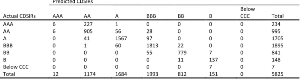
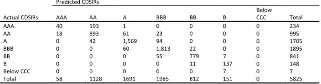
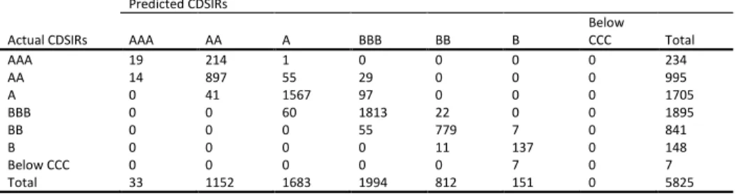
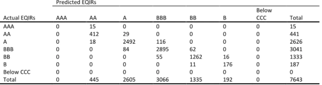
5.1AccuracyIn Table 6 we evaluate the forecasts of the models under study for firms’ CDSIRs and EQIRs, using Accuracy Ratios (ARs). The AR related to the percentage of correct forecast is the sum
of all diagonal terms divided by the total number of observations in each contingency table (see Appendix B) 𝐴𝑅 =1𝑇∑𝑡=1𝑇 1(𝑞̂𝑡= 𝑞𝑡) where 𝑞̂𝑡 denotes the predicted rating and 𝑞𝑡 represents the actual outcome. We report statistics for all candidate models for both in- and out-of-sample predictions. For the out-of-sample predictions of ratings we use the past and current information available up to time 𝑇. We use an expanding window method, which allows the successive observations to be included in the initial sample prior to forecast of the next one-step ahead prediction of the rating while keeping the start date of the sample fixed. By this method, we forecast future ratings 𝑞̂𝑡+1, 𝑞̂𝑡+2 etc. The initial estimation window is 2002 to 2005 and the first prediction date is year 2006. We then increase 𝑇 by one each time until 𝑇 reaches year 2008. In addition, we report at the foot of each panel the number of surviving variables15.
Insert Table 6
To begin with the in-sample exercise, we find no notable differences between the competing models since they present a similar in-sample performance for both types of market implied ratings. With respect to CDSIRs, approximately 90% predictions are correct, while for EQIRs we find that the models have approximately 95% correct predictions. Moving to the out-of-sample prediction, the results suggest that the LASSO models clearly outperform their OP benchmark. When considering the CDSIRs, our results indicate that the percentage of correct predictions increase from 22% in the OP model to 84% in the LASSO models. With reference to EQIRs, the percentage of correct predictions improves from 49% in the OP model to 91% in the LASSO models.
Next, we compare the within performance of the LASSO models, by considering alternative LASSO specifications. Starting with CDSIRs, the models with BIC-type tuning parameter selector provide more accurate out-of-sample forecasts compared to the LASSO models with AIC-type tuning parameter selector. For EQIRs, there is little difference in the accuracy ratios of the various LASSO candidate models.It is interesting to note that the LASSO models with BIC-type tuning parameter selector select consistently a smaller number of predictors than
15 The surviving variables are defined as predictors with non-zero estimated coefficients after the penalized
procedure. In the benchmark model, we do not drop any variables since OP does not penalise regression coefficients.
20 their AIC-type counterparts. This does not seem to affect their forecasting performance for EQIRs but leads to more accurate predictions for CDSIRs.16
5.2 Statistical significance
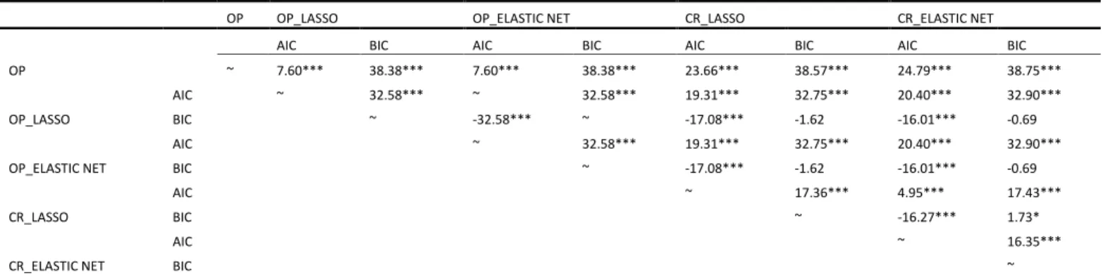
To evaluate the relative performance of the models presented in the sub-section above, we employ the Stuart–Maxwell test. This approach will help us formally test for the statistical significance of the difference between forecasts and to further validate our main findings. The Stuart–Maxwell test (Stuart, 1955; Maxwell, 1970) is a generalized version of McNemar’ test (McNemar, 1947), which is associated with multiple (𝑘) categories and tests whether the difference between two related samples from an ordinal field is statistically different from zero. The Stuart–Maxwell tests the null hypothesis of equal marginal proportion for each category between the forecasts of two models (model A vs model B). Under the null hypothesis, the statistic is distributed as chi-square with 𝑘 − 1 degrees of freedom. A statistically significant Stuart–Maxwell test statistic indicates that the forecasts of the first model (A) are different from those of the second model (B).
For the CDSIRs, as can be seen from Table 6, there is evidence of a statistically significant difference in out-of-sample predictions between the OP model and other competing models. For the EQIRs, the results of the out-of-sample forecasts paint a very similar picture. However, this tendency cannot be clearly observed in the in-sample forecasts of all competing models for both CDSIRs and EQIRs. Combing these statistics with the accuracy ratios, it can be confirmed that adding LASSO or the Elastic net estimator in the OP model or the CR model, can produce different out-of-sample forecasts that are more accurate than those generated by the OP.
5.3Robustness tests
The findings of the previous Section are further validated by carrying-out several robustness tests. In the first test, we consider an alternative choice of tuning parameters by using the
16 Tables B1 to B36 in on-line Appendix B illustrate the contingency tables of the predicted against the actual
cross validation. Next, we rely on an alternative benchmark for forecasting, namely the Principal Component Analysis. In a further test we employ a tuning-free version of the LASSO estimator. As a fourth test, we use alternative measures of predictive ability. Furthermore, we allow only investment grade ratings. Finally, we consider random effects in panel data.
5.3.1 Cross validation
It is well accepted that the choice of tuning parameter is crucial for the finite-sample performance of estimators such as LASSO or elastic net. Motivated by this consideration, we present forecasts when cross validation is employed, which is one of the most commonly used model selection criteria (see for instance, Stone, 1974 and Yang, 2007). Specifically, we use the ten-fold stratified cross validation (10-fold CV) as a general application of tuning parameter selector. This choice is in line with the relevant literature of model selection (see for example, Kohavi, 1995).
Insert Table 7
The Accuracy Ratios and Stuart–Maxwell test statistics, presented in Table 7, corroborate our main findings. In the in-sample forecast exercises, all models present similar predictive ability. In the out-of-sample prediction, however, for the CDSIRs, all competing LASSO models provide more accurate forecasts than the benchmark model. This tendency can be also observed in the EQIRs. In sum, it appears that there are significant gains in predictive ability once the LASSO is applied even when cross validation is employed. We conclude that our main results are robust to alternative tuning choices.
5.3.2 Principal Component Analysis with OP
One of the most popular statistical procedures for variable selection is the Principal Component Analysis (PCA). PCA converts a set of possibly correlated variables to a smaller set of uncorrelated variables called Principal Components (PC). The first PC accounts as much of the variability in the dataset as possible and each succeeding component turn attains the highest variance possible under the constraint that it is orthogonal to the preceding
22 components. PCA is probably the most popular dimension reduction procedure in Economics and Finance and has been applied successfully to a series of forecasting problems (see Stock and Watson, 2002, Ludvigson and Ng, 2009 and Bailey et al, 2016). In our application, we are dealing with a large set of possibly correlated variables and thus a natural candidate to benchmark our procedure is the PCA. We select the PCs that account of the 70%, 80% and 90% of the variability in our dataset and combine them with OP. The relevant accuracy ratios are presented in Table 8.
Insert Table 8
Comparing Tables 8 and 6 (where the accuracy ratios of OP and OP with LASSO are presented), we note that PCA naturally improves the out-of-sample accuracy of the single OP model. For our OP combined with LASSO models, the only case that PCA manages to beat our models in terms of out-of-sample accuracy is for CDSIRs. In that case, OP based on the PCs that explain the 70% and 90% of the variability, present a higher accuracy ratio compared to LASSO model with AIC-type tuning parameter selector (but not under the BIC-type selector). It is also interesting to note that PCA with OP displays lower in-sample accuracy ratios at all cases. These results allow to argue that our LASSO formulations are robust to an alternative benchmark.
5.3.3 A tuning-free version of the LASSO
While the results presented so far are robust to different tuning choices, including cross validation, it is important to note that the latter is computationally costly and theoretically less well developed, especially for the purpose of variable selection and the estimation of regression coefficients (see Sun and Zhang, 2012). Thus, to further alleviate potential concerns regarding the choice of the tuning parameter, we employ the scaled LASSO, developed by Sun and Zhang (2012), without depending on model selection criteria such as AIC, BIC or CV1718.
Insert Table 9
17 Another tuning-free version of the LASSO estimator is the square-root LASSO by Belloni et al. (2011). 18 For the scaled LASSO, the authors generated the gradient descent algorithm in a convex minimization of a
Table 9 presents the relevant Accuracy Ratios and the realizations of the Stuart–Maxwell statistical tests. We note that on in-sample evidence all models continue to display similar accuracy. In the out-of-sample evaluation, for the CDSIRs and EQIRs the predictive performance of the scaled LASSO is superior compared with that of the OP. Once again, this finding is consistent with our main results, indicating that our findings are robust to using the scaled LASSO.
5.3.4 Alternative measures of predictive ability 5.3.4.1
Thus far, the relative performance of the estimated models is evaluated in terms of an informal goodness of fit indicator, by comparing predicted and observed ratings. It is possible, however, to give a more quantitative measure of the predictive ability of our models. We therefore check the robustness of our measure of predictive power by using a measure based on a technique proposed by Merton (1981) and used in Henriksson and Merton (1981), Pesaran and Timmermann (1994), Kim et al. (2008) and Mizen and Tsoukas (2012). Specifically, let 𝐶𝑃𝑗 be the proportion of the correct predictions made by 𝑞̂𝑡 when the true state is given by 𝑞𝑡 = 𝑗. From the definition of conditional probability, 𝐶𝑃 is computed as 𝐶𝑃𝑗= 1
𝑇∑𝑇𝑡=11(𝑞̂𝑡=𝑗)(𝑞𝑡=𝑗) 1
𝑇∑𝑇𝑡=11(𝑞𝑡=𝑗) and the Merton’s correct measure expressed 𝐶𝑃 is given by 𝐶𝑃 = 1
𝐽−1[∑ 𝐶𝑃𝑗 𝐽
𝑗=1 − 1] where 𝐽 is the number of categories, and − 1
𝐽−1< 𝐶𝑃 < 1. In the contingency table (see Appendix B) 𝐶𝑃 is the unweighted average of 𝐶𝑃𝑗s minus one (to correct for the phenomenon that certain categories are over-represented). The 𝐶𝑃𝑗s are calculated as the proportion of correct predictions divided by the total of each row. This modifies the measure of predictive ability to discount the influence of the dominant outcome. A high 𝐶𝑃 score indicates that the predictor is accurate for all rating categories.
Insert Table 10
The Accuracy Ratios when we account for the influence of the dominant outcome by reporting the Merton correct predictions are shown in Table 10. We also report the corresponding Stuart–Maxwell statistical tests. The test produces 𝐶𝑃 ratios that confirm our
24 main findings. In the in-sample exercise, there is little difference between the OP and the LASSO models. In contrast, the predictive ability of the out-of-sample predictions is superior when penalty functions are applied.
5.3.4.2
An alternative measure for our forecasts can be constructed based on the misclassification rate of Hastie et al. (2009): 𝑇−1∑𝑇𝑡=11{𝑞̂ ≠ 𝑞𝑡 𝑡} . In the spirit of Diebold and Mariano (1995),
we estimate the misclassification rate for each forecast and then we test if the mean difference of these rates between two models is 0 or not. If this difference is statistically different than 0, then this mean that the two models generate different forecasts. Tables 11 and 12 presents the relevant p-values for our out-of-sample forecasts.
Insert Tables 11 Insert Tables 12
We note that in almost all cases, our forecasts are statistically different. These results supplement the previous section and further demonstrate the superiority of LASSO as a variable selection technique and the effectiveness of BIC criterion in tuning the LASSO parameters. To sum up, the results are robust to using a test that calculates correct predictions using the proportion of correct predictions for each of the various rating categories.
5.3.5 Investment grade ratings
Much of the previous related literature studies employ data with investment grade ratings. However, as noted by Amato and Furfine (2004), restricting attention to one category is likely to induce selection bias. On the other hand, pooling together both categories may result in misspecification of our model if changes in financial and business risk have a different impact on creditworthiness across the groups of firms. Therefore, we drop all speculative grade ratings and re-estimate our models.
The results in Table 13 corroborate our main findings. In the in-sample forecast exercises, all models present similar performance. For the CDSIRs, both versions of the CR with LASSO provide more accurate forecasts. On the other hand, for EQIRs all LASSO models display better predictive performance than their OP benchmark. To sum up, even when limiting our sample to investment grade ratings only, the out-of-sample predictions evidence that the LASSO models outperform the benchmark model.
5.3.6 Accounting for the panel data dimension
As a final robustness test we consider a random-effects version of the ordered probit model to take into account the panel data dimension of the data-set. The Accuracy Ratios and the corresponding Stuart–Maxwell statistical tests are reported in Table 14. As can be seen, the main findings remain unchanged: when we apply the LASSO or Elastic net estimator the models have superior predictive ability compared to the ordered probit model, even when random effects are included. We conclude that our findings are robust to estimating the models with random effects to deal with the panel data nature of the sample.
Insert Table 14
5.4 Discussion
In the previous Sections, a forecasting exercise on CDSIRs and EQIRs prediction is presented. For both types of market implied ratings all models present similar in-sample accuracy. In the out-of-sample evaluation, for CDSIRs, we observe the LASSO models controlled by BIC-type tuning parameter selector outperform their benchmarks. We also observe that these models, select a smaller number of surviving variables than their counterparts with the AIC-type selector. This lends support to the argument that the models with BIC-type tuning parameter selectormake better use of the available information. For the EQIRs, we note a similar pattern. The models with the BIC-type tuning parameter selector outperform their counterparts with the AIC-type selector in terms of accuracy while at the same time they select a smaller number of variables.
26 To sum up, we note that the LASSO models are able to provide more accurate out-of-sample forecasts on the CDSIRs and EQIRs ratings that outperform the OP model. This is of particular interest given that the OP model dominates the related literature in predicting credit ratings. From the LASSO models under study, the optimized models with BIC-type tuning parameter selector seem able to provide better forecasts while at the same time they use less predictors. These results are robust to modifying the tuning parameters, to considering a tuning-free version of LASSO, to evaluating the predictive performance of the models using a different statistical measure and to restricting the dataset to investment grade ratings.
6 Conclusion
The ability to predict credit ratings within a reasonable margin of accuracy is of vital importance for both market participants and rating agencies. The focus on market implied ratings is even more justified as long-term ratings have been heavily criticized about their performance during the recent global financial crisis. We model the prediction of market implied ratings applying a variable selection technique, the least absolute shrinkage and selection operator (LASSO), and its most promising derivation, the Elastic net, into ordered probit and continuation ratio models.All LASSO models select the most relevant predictors from a set of 268 variables and forecast the MIRs for a period of six years (2002 to 2008). This marks a break with the existing literature which typically relies on discrete limited dependent variable models.
Our results using monthly data from the US offer several interesting results. First, we show that financial factors along with market-driven and macroeconomic variables contain information about market implied ratings. Second, the LASSO models perform better in out-of-sample prediction than do ordered probit models, mostly adopted in previous studies. Finally, the optimized LASSO models with BIC-type tuning parameter selector outperform their counterparts with AIC-type selector for the dataset and periods under study. Hence, LASSO-selected models attain an improved forecasting power.
These results should go further in convincing risk managers and academics to explore variable selection models when assessing credit risk. The structure of credit ratings is unknown and likely to vary through time. Limited dependent variable models require a-priori knowledge on the explanatory variables set, which can lead to misspecifications. On the other hand, variable selection models such as LASSO, are more flexible and can unveil the underlying structure of the problem leading to superior estimations and improved predictive ability.
References
Akaike, H. (1974). A New Look at the Statistical Model Identification. IEEE Transactions on Automatic Control, 19(6), pp.716-723.
Altman, E. (1968). Financial Ratios, Discriminant Analysis and the Prediction of Corporate Bankruptcy. The Journal of Finance, 23(4), p.589.
Archer, K. and Williams, A. (2012). L1 Penalized Continuation Ratio Models for Ordinal Response Prediction Using High-Dimensional Datasets. Statistics in Medicine, 31(14), pp.1464-1474.
Amato, J. and Furfine, C. (2004). Are Credit Ratings Procyclical?. Journal of Banking & Finance, 28(11), pp.2641-2677.
Amendola, A., Restaino, M. and Sensini, L. (2011). Variable Selection in Default Risk Models. The Journal of Risk Model Validation, 5(1), pp.3-19.
Bailey, N., Holly, S. and Pesaran, M. H. (2016). A Two‐Stage Approach to Spatio‐Temporal Analysis with Strong and Weak Cross‐Sectional Dependence. Journal of Applied Econometrics, 31(1), pp. 249-280.
Breger, L., Goldberg, L. and Cheyette, O. (2003). Market Implied Ratings. Risk Magazine, pp.85-89.
Belloni, A., Chernozhukov, V., and Wang, L. (2011). Square-root lasso: pivotal recovery of sparse signals via conic programming. Biometrika, 98(4):791–806.
Blume, M., Lim, F. and Mackinlay, A. (1998). The Declining Credit Quality of U.S. Corporate Debt: Myth or Reality?. The Journal of Finance, 53(4), pp.1389-1413.
Castellano, R. and Giacometti, R. (2012). Credit Default Swaps: Implied Ratings Versus Official Ones. 4OR, 10(2), pp.163-180.
Chava, S. and Jarrow, R. (2004). Bankruptcy Prediction with Industry Effects. European Finance Review, 8(4), pp.537-569.
Contoyannis, P., Jones, A. and Rice, N. (2004). The Dynamics of Health in the British Household Panel Survey. Journal of Applied Econometrics, 19(4), pp.473-503.
28 Creal, D., Gramacy, R. and Tsay, R. (2014). Market-Based Credit Ratings. Journal of Business &
Economic Statistics, 32(3), pp.430-444.
Diebold, F. and Mariano, R. (1995). Comparing Predictive Accuracy. Journal of Business & Economic Statistics, 13(3), p.253.
Doumpos, M., Niklis, D., Zopounidis, C. and Andriosopoulos, K. (2015). Combining Accounting Data and a Structural Model for Predicting Credit Ratings: Empirical Evidence from European Listed Firms. Journal of Banking & Finance, 50, pp.599-607.
Duffie, D., Saita, L. and Wang, K. (2007). Multi-Period Corporate Default Prediction with Stochastic Covariates. Journal of Financial Economics, 83(3), pp.635-665.
Ederington, L. (1985). Classification Models and Bond Ratings. The Financial Review, 20(4), pp.237-262.
Efron, B., Hastie, T., Johnstone, I. and Tibshirani, R. (2004). Least Angle Regression. The Annals of Statistics, 32(2), pp.407-499.
Fan, J. and Li, R. (2001). Variable Selection via Nonconcave Penalized Likelihood and its Oracle Properties. Journal of the American Statistical Association, 96(456), pp.1348-1360. Fienberg, S. E. (1980) The Analysis of Cross-Classified Categorical Data. Cambridge, MA: The
MIT Press.
Fitch (2007) Fitch CDS Implied Ratings Model. Available at: https://www.fitchratings.com/web_content/product/methodology/cdsir_methodology .pdf (Accessed: 20 October 2016).
Gentry, J., Whitford, D. and Newbold, P. (1988). Predicting Industrial Bond Ratings with a Probit Model and Funds Flow Components. The Financial Review, 23(3), pp.269-286. Güttler, A. and Wahrenburg, M. (2007). The Adjustment of Credit Ratings in Advance of
Defaults. Journal of Banking & Finance, 31(3), pp.751-767.
Hastie, T., Tibshirani, R. and Friedman, J. (2009). The Elements of Statistical Learning: Data Mining, Inference and Prediction. Springer, 2nd ed. New York: Springer, pp.219-221. Härdle, W. and Prastyo, D. (2013). Default Risk Calculation Based on Predictor Selection for
the Southeast Asian Industry. SSRN Electronic Journal.
Hardin, J.W., Hilbe, J.M. and W, H. (2007) Generalized Linear Models and Extensions. 2nd edn. College Station, TX: Stata Press.
Henriksson, R. and Merton, R. (1981). On Market Timing and Investment Performance. II. Statistical Procedures for Evaluating Forecasting Skills. The Journal of Business, 54(4), p.513.
Horrigan, J. (1966). The Determination of Long-Term Credit Standing with Financial Ratios. Journal of Accounting Research, 4, p.44.
Hwang, R. (2011). Predicting Issuer Credit Ratings Using Generalized Estimating Equations. Quantitative Finance, 13(3), pp.383-398.
Hwang, R. (2013). Forecasting Credit Ratings with the Varying-Coefficient Model. Quantitative Finance, 13(12), pp.1947-1965.
Hwang, R., Cheng, K. and Lee, C. (2009). On Multiple-Class Prediction of Issuer Credit Ratings. Applied Stochastic Models in Business and Industry, 25(5), pp.535-550. Hwang, R., Chung, H. and Chu, C. (2010). Predicting Issuer Credit Ratings Using a
Semiparametric Method. Journal of Empirical Finance, 17(1), pp.120-137.
Kao, C. and Wu, C. (1990). Two-Step Estimation of Linear Models with Ordinal Unobserved Variables: The Case of Corporate Bonds. Journal of Business & Economic Statistics, 8(3), p.317.
Kaplan, R. and Urwitz, G. (1979). Statistical Models of Bond Ratings: A Methodological Inquiry. The Journal of Business, 52(2), p.231.
Kim, T., Mizen, P. and Chevapatrakul, T. (2008). Forecasting Changes in UK Interest Rates. Journal of Forecasting, 27(1), pp.53-74.
Kohavi, R. (1995). A Study of Cross-Validation and Bootstrap for Accuracy Estimation and Model Selection. Proceedings of the 14th international joint conference on Artificial intelligence, 2, pp.1137-1143.
Liu, B., Kocagil, A.E. and Gupton, G.M. (2007) Fitch Equity Implied Rating and Probability of
Default Model. Available at:
https://www.fitchratings.com/web_content/product/methodology/eir_methodology.p df (Accessed: 20 October 2016).
Long, S.J. and Freese, J. (2006) Regression Models for Categorical Dependent Variables Using Stata. 2nd edn. College Station, TX: StataCorp LP.
Ludvigson, S. C. and Ng, S. (2009). Macro Factors in Bond Risk Premia. The Review of Financial Studies, 22(12), pp.5027–5067.
Maddala, G. (2008). Limited-Dependent and Qualitative Variables in Econometrics. Cambridge: Cambridge Univ. Press, pp.47-48.
Maxwell, A. (1970). Comparing the Classification of Subjects by Two Independent Judges. The British Journal of Psychiatry, 116(535), pp.651-655.
McNemar, Q. (1947). Note on the Sampling Error of The Difference Between Correlated Proportions or Percentages. Psychometrika, 12(2), pp.153-157.
Merton, R. (1981). On Market Timing and Investment Performance. I. An Equilibrium Theory of Value for Market Forecasts. The Journal of Business, 54(3), p.363.
Mizen, P. and Tsoukas, S. (2012). Forecasting US Bond Default Ratings Allowing for Previous and Initial State Dependence in an Ordered Probit Model. International Journal of Forecasting, 28(1), pp.273-287.
Ohlson, J. (1980). Financial Ratios and the Probabilistic Prediction of Bankruptcy. Journal of Accounting Research, 18(1), p.109.
30 Pesaran, M. and Timmermann, A. (1994). A Generalization of the Non-Parametric
Henriksson-Merton Test of Market Timing. Economics Letters, 44(1-2), pp.1-7.
Pinches, G. and Mingo, K. (1973). A Multivariate Analysis of Industrial Bond Ratings. The Journal of Finance, 28(1), pp.1-18.
Pogue, T. and Soldofsky, R. (1969). What's in a Bond Rating. The Journal of Financial and Quantitative Analysis, 4(2), p.201.
Poon, W. (2003). Are Unsolicited Credit Ratings Biased Downward?. Journal of Banking & Finance, 27(4), pp.593-614.
Rösch, D. (2005). An Empirical Comparison of Default Risk Forecasts from Alternative Credit Rating Philosophies. International Journal of Forecasting, 21(1), pp.37-51.
Schwarz, G. (1978). Estimating the Dimension of a Model. The Annals of Statistics, 6(2), pp.461-464.
Shao, J. (1997). Am Asymptotic Theory for Linear Model Selection. Statistica Sinica, 7(2), pp.221-242.
Shumway, T. (2001). Forecasting Bankruptcy More Accurately: A Simple Hazard Model. The Journal of Business, 74(1), pp.101-124.
Stock, J. H. and Watson, M. W. (2002). Forecasting using principal components from a large number of predictors. Journal of the American statistical association, 97(460), pp.1167– 1179.
Stone, M. (1977). An Asymptotic Equivalence of Choice of Model by Cross-Validation and Akaike's Criterion. Journal of the Royal Statistical Society. Series B (Methodological), 39(1), pp.44-47.
Stuart, A. (1955). A Test for Homogeneity of the Marginal Distributions in a Two-Way Classification. Biometrika, 42(3/4), p.412.
Sun, T. and Zhang, C. (2012). Scaled Sparse Linear Regression. Biometrika, 99(4), pp.879-898. Tian, S., Yu, Y. and Guo, H. (2015). Variable Selection and Corporate Bankruptcy
Forecasts. Journal of Banking & Finance, 52, pp.89-100.
Tibshirani, R. (1996). Regression Shrinkage and Selection via the Lasso. Journal of the Royal Statistical Society. Series B (Methodological), 58(1), pp.267-288.
Tsoukas, S. and Spaliara, M. (2014). Market Implied Ratings and Financing Constraints: Evidence from US Firms. Journal of Business Finance & Accounting, 41(1-2), pp.242-269. van de Geer, S. (2008). High-Dimensional Generalized Linear Models and The Lasso. The
Annals of Statistics, 36(2), pp.614-645.
West, R. (1970). An Alternative Approach to Predicting Corporate Bond Ratings. Journal of Accounting Research, 8(1), p.118.