Creating a More Efficient Course Schedule at WPI Using Linear Optimization

Project Number: ACH1211

Creating a More Efficient Course Schedule at

WPI Using Linear Optimization

A Major Qualifying Project Report submitted to the Faculty

of the

WORCESTER POLYTECHNIC INSTITUTE in partial fulfillment of the requirements for the

Degree of Bachelor of Science by

Ryan Wormald

Curtis Guimond

Date: April 26, 2012 Approved:

Dean Arthur C. Heinricher, Advisor

Abstract

The current course scheduling process at Worcester Polytechnic Institute often results in an ineffi-cient assignment of courses to classrooms due to the manual work, and other challenges, involved. The goal of this project was to develop a mathematical model and a software tool that will help WPI develop a more efficient course schedule. By creating this software tool, the process of course scheduling was automated, and an improved course schedule was produced. The program allows for the integration of changes in schedule information, as well as flexibility and future expansion of the model.

Authorship

Ryan Wormald: Formulation of global and local problems, formulation of algorithm for adding a new course to a current schedule, writing Matlab code for automating the process of creating a more efficient schedule, analysis of efficiency output in Matlab, development of the occupation matrices, writing Matlab code for adding a new course, reformatting schedule data in Excel, back-ground research on linear programming and network flow, writing and editing report

Curtis Guimond: Formulation of global and local problems, formulation of algorithm for adding a new course to a current schedule, background research on course scheduling, timetabling, and network flow, writing and editing report

Acknowledgments

We would like to thank our advisors, Dean Arthur Heinricher and Professor Suzanne Weekes, for their guidance and support throughout the completion of this project. We would also like to thank Chuck Kornik for his willingness to assist with this project. Lastly, we would like to thank Dave Galvin for providing the current course schedule data, Adriana Hera for her assistance with Matlab, and all other WPI faculty members who assisted us throughout the course of this project.

Contents

1 Introduction 3

2 Background: Mathematics Behind Scheduling 5

2.1 Linear Programming . . . 5

2.1.1 Integer Linear Programming . . . 8

2.2 Network Flow . . . 8

2.2.1 Minimum Cost Flow Problem . . . 9

2.2.2 Assignment Problem . . . 12

2.2.3 Network Simplex Method . . . 13

3 Background: Course Scheduling 17 3.1 Applications of Course Scheduling . . . 17

3.1.1 Course Timetabling . . . 19

4 Project Formulation 21 4.1 Global Scheduling Problem . . . 22

4.2 Local Scheduling Problem . . . 24

4.3 Data Processing . . . 24

4.4 Optimization . . . 26

4.4.1 Occupation Matrix . . . 26

4.4.2 Model . . . 28

4.4.3 Update . . . 29

4.5 Adding a New Course . . . 30

5 Results and Analysis 31 6 Conclusions 34 6.1 Recommendations . . . 35

7 Appendix A: Steps for Reformatting Data in Excel 38

8 Appendix B: Lookup Tables for Indexing in Excel 40

10 Appendix D: Matlab Code for Adding New Courses 56

List of Figures

2.1 Network for Minimum Cost Flow Example . . . 10

2.2 Initial Network Solution - with cost and supply/demand values . . . 14

2.3 Initial Network Solution - with primal flow, dual, and dual slack values . . . 16

4.1 Schedule for Calculus I (only lectures) . . . 22

4.2 Occupation Matrix Displaying Number of Sections . . . 27

4.3 Occupation Matrix Displaying Course Populations . . . 28

4.4 Occupation Matrix Displaying Efficiencies . . . 28

5.1 Efficiency Output From Matlab . . . 33

List of Tables

2.1 Primal and Dual Formulation Rules . . . 7 4.1 Column Data From Excel Spreadsheet . . . 25 5.1 Changes in Efficiency for MTRF Schedule Type Blocks . . . 32

Executive Summary

The current scheduling system at WPI starts with the previous academic years schedule and adjusts it to accommodate changes. The system assigns over 3000 course meetings into 83 schedulable spaces at 14 different times. However, the schedules produced are not always efficient. For ex-ample, a course may be assigned to a classroom with a capacity much greater than the student population.

The goal of this project is to develop a mathematical model and a software tool that will help WPI develop a more efficient schedule. The efficiency of a course-room pair is defined as the ratio of the course population limit to the room capacity; if the course population exceeds a room capac-ity, however, the efficiency is defined to be zero. The total efficiency of a schedule is a weighted sum of the efficiencies for each course-room pair. The weight of a course-room pair is termed its happiness coefficient, which reflects a penalty or reward given to a course being assigned to a certain room. For example, a music course has a high happiness coefficient when assigned to rooms in Alden Hall, but a coefficient of zero when assigned to Goddard Labs.

The model starts with an initial schedule exported from Banner into an Excel spreadsheet. The data includes information about each courses lectures, conferences, and labs, such as start and end times, course populations, and classroom assignments. The data is then imported into Matlab to be used for optimization.

There is a global linear programming problem associated with the optimization of the schedule as a whole. The objective of this problem is to maximize the efficiency of a schedule subject to a set of constraints, which do not allow (i) more than one course to be held in the same classroom at the same time and (ii) more than one classroom to be paired with the same course at one time. This problem enables courses to change from previously assigned times and schedule types. This global linear program (LP) is NP-hard, referring to the complexity of the problem.

The global problem was then simplified by adding constraints and separating the problem into local linear programs (LPs). Each local LP is associated with a block, which is defined as a set of courses that has the same schedule type, start time, and duration time. Examples of blocks would be hour-long courses held on MTWRF at 9am or two-hour long classes held on MR at noon. The objective of each local LP is to maximize the efficiency of an individual block. The local LPs also restrict time and schedule type from being changed, whereas the global LP does not. By solving a

sequence of local LPs associated with each individual block, we can improve the efficiency of the schedule.

The final model allows for improvement in the efficiency of the schedule by optimizing the sequence of local LPs. In addition, an occupation matrix was generated from our model, which contains the percentage of seats used in each schedulable room at every available day and hour. The model also has the ability to be easily expanded in the future. In the end, a mathematical model was created for course scheduling that can be implemented to improve the assignments of courses in the current schedule as well as enable changes to be made more easily.

Chapter 1

Introduction

Course scheduling continues to be a large, unsolved problem at all universities. Course scheduling for this project refers to the administrative aspects of course scheduling, such as assigning courses to rooms and times. There are many resources involved in the scheduling process, such as students, rooms, teachers, and buildings. Currently, there is no way to find an ”optimal” schedule given the many restrictions and preferences on room assignments. These restrictions and preferences regard the use of blackboards vs. whiteboards, having rooms equipped with course capturing equipment, or being located in a handicapped accessible building.

For these reasons, many universities have solved subproblems, where the goal is to improve the current schedule as opposed to finding the optimal solution. Similar to other universities, Worces-ter Polytechnic Institute is also faced with this complex scheduling problem. There are software packages, which can solve (approximately) simpler versions of the problem.

The student population of WPI has been constantly increasing. This past year, the enrollment number increased from 3,537 in 2010-11 [13] to 3,746 undergraduate students in 2011-12 [12]. In order to accommodate this number of undergraduates, as well as the graduate students enrolled, there were a total of 433 course sections offered in A term, 2011. This is a 10.7% increase from the 391 course sections offered in A term of the previous year. To offer all of these sections, nine academic buildings are utilized on campus with a total of 41 classrooms and nine computer labs, which are used as classrooms as needed. There are several other spaces used on campus as well, such as music rooms in Alden Hall and the athletic field. The classrooms range in size from 25 seats in the smallest room to 220 in the largest. In total for this project, there is approximately 3,000 meetings to be scheduled in 83 schedulable rooms within 14 time slots throughout the 2011-12 academic year [8].

There are several steps in the scheduling process that are followed each year to create the schedule for the next year. This process is guided by Chuck Kornik, Administrator of Academic Programs.

changes need to be made to satisfy faculty preferences and other constraints.

Step 2 (February): Using the previous year’s schedule as a basis, changes are made according to the results in Step 1.

This scheduling process begins each January when each department head is surveyed. They are required to fill out a sheet with course changes for the next year, such as adding or dropping a course or section or changing the term or time a course is offered. These surveys are due back to Chuck Kornik by February, who then uses the previous year’s schedule to build the new schedule. Changes are made to this schedule according to each department head survey. Each course section is then placed into a classroom and time slot. Times for Calculus I-IV, Physics I-IV, Chemistry I-IV, Introduction to Program Design, and Accelerated Introduction to Program Design remain un-changed. These times were set several years ago in order to avoid time conflicts. Each of these courses is a basic requirement for most majors; therefore, a high population of students takes one or more during one term.

By March, the new schedule is finalized. This schedule is given to each department head, who may request any necessary changes. Adjustments are made to the schedule, such as adding more sections to a course or changing the time of a course. This must all be done by mid-April when course registration opens for undergraduates. Additional changes may be needed after students register to accommodate shifts in demand or waitlists.

With this current scheduling process, some courses may be placed into rooms too large for the number of students enrolled in the course. For example, there is currently a physics conference with 26 students held in Olin Hall 107, which seats 202 students. Only 12.87% of the classroom space is utilized during these conference times. This would be considered an inefficient course to classroom assignment, where efficiency is measured by the percentage of classroom space occu-pied by a course assigned to it.

Some other challenges that arise during scheduling are: 1. adding new courses to the current schedule;

2. sudden changes to course information, such as the population limit of the course;

3. moving courses to new rooms and/or times because of special needs of instructor or student, for example.

An automated scheduling system would help in facing these challenges more readily. While the problem of finding an optimal schedule is complex, or unsolvable, smaller subproblems that can be solved to improve the current schedule.The goal of this project is to develop a mathematical model and a software tool that will enable WPI to develop a more efficient course schedule, while addressing the challenges that were highlighted above.

Chapter 2

Background: Mathematics Behind

Scheduling

There are several methods of mathematics involved in dealing with a course scheduling problem. Examples include linear programming and network flow. Therefore, it is helpful to understand some of the mathematics used behind course scheduling models.

2.1

Linear Programming

In creating a mathematical model for course scheduling, it is important to first understand the method of linear programming. Linear programming is used in mathematical optimization when a linear function, called the objective function, is maximized (or minimized) subject to a set of linear constraints. The objective function and constraints are written in terms of decision variables, which are the variables that define the solution. Common linear programming problems maximize the profit of a company or minimize the production cost subject to constraints such as a limit on how much material or time or money is available.

Solutions of a linear program which satisfy all constraints in the problem are called feasible solutions. These solutions do not necessarily optimize the objective value. An optimal solution is one that satisfies the constraints, as well as optimizes the objective function. If there is no solution that satisfies all constraints, then the problem is called infeasible.

The standard form of a linear program is Maximize:

n

∑

Subject to: n

∑

wherexj are the decision variables,cj are the cost coefficients, andbi are the limits on each

con-straint.

Written in matrix form, the standard form becomes

Maximize:c|x Subject to:Ax_≤b

x_≥0

This is known as the primal problem of the linear program. There are a total ofmconstraints and

ndecision variables, and the decision variables,x= [xj], and the cost coefficients,c= [cj], are in

the form of column vectors of sizen×1. The right hand side values, b= [bi], are in the form of a

column vector of sizem_×1. The matrixA= [ai j]is anm×nmatrix.

Associated with every linear programming problem is another problem known as the dual. The standard form for the dual is shown below.

Minimize: m

∑

∑

Written in matrix form, the standard form is

Minimize: b|y Subject to:A|_y≥c

y_≥0

where the decision variables of the dual, y= [yi] is in the form of a column vector. A feasible

∑

cjxj≤

∑

biyi

where x is a feasible solution to the primal and y is a feasible solution to the dual. This is the Weak Duality Theorem [11]. The Strong Duality Theorem states that, when solutions to both the primal and dual are equal to each other, then that is the optimal solution of the linear programming problem. That is,

∑

cjx∗j =

∑

biy∗i

wherex∗is the optimal solution to the primal andy∗is the optimal solution to the dual.

There are simple rules to help find the dual problem, which are given in Table 2.1 below. These rules can be used when for a primal problem in any form, not just standard form. Constraints and variables in the primal, shown in the left side of the table, determine what type of constraints and variables will be in the dual, shown in the right side of the table. For example, if constrainti in the primal problem is an equality, variableyiin the dual will be a free variable. Free variables are

variables that are unrestricted in bound.

Primal Dual

Equality Constraint Free Variable Inequality Constraint Nonnegative Variable

Free Variable Equality Constraint Nonnegative Variable Inequality Constraint Table 2.1: Primal and Dual Formulation Rules

To understand the concepts outlined above, consider an example of a linear programming prob-lem shown below [11]:

Maximize: x1−2x2 Subject to: x1 +2x2 −x3 +x4 ≥0 4x1 +3x2 +4x3 −2x4 ≤3 −x1 −x2 +2x3 +x4 =1 x2,x3≥0 x1,x4free

Using the table for primal and dual rules, the dual of this problem is as follows: Minimize: 3y2+y3 Subject to: y1 +4y2 −y3 =1 2y1 +3y2 −y3 ≥ −2 −y1 +4y2 +2y3 ≥0 y1 −2y2 +y3 =0 y1≤0 y2≥0 y3free

There are several different algorithms used for solving linear programs, the most common one being the simplex method. During each iteration of this algorithm, a feasible solution is produced. The algorithm is iterated until the optimal solution is obtained [11].

2.1.1

Integer Linear Programming

Different conditions can be imposed on linear programming problems to allow to model real-world problems. Similar to linear programming is integer linear programming. An integer linear program takes the same form as the linear programming model above, but with one addition: the decision variables are constrained to being integers [10]. In some cases, only some variables are constrained to being integers; this problem is call a mixed integer programming problem. Another type of in-teger programming is called 0-1, or binary, inin-teger programming. This is the case in which all decision variables must be either 0 or 1. Integer programming is common in real-world problems, such as shipping problems, in which items must be shipped in one piece. Fractions of an item being shipped to separate locations would be unrealistic.

Linear programming has a wide range of applications and extensions and can be applied to a wide variety of real-world situations, including the problem of scheduling courses. In focusing on the course scheduling problem at hand, it is important to look closely at another particular type of example, known as network flow problems.

2.2

Network Flow

Networks are used in many industries, such as the transportation and shipping industries. These networks are used to solve problems regarding production, distribution, and much more. There are several different types of network optimization problems; one type that will be discussed is the minimum cost flow problem. This type of network flow problem provides a basis for most other types of network flow problems. Another type of network flow problem that will be discussed in

2.2.1

Minimum Cost Flow Problem

To understand a network flow model, some key terms must be defined. First, a network consists of nodes and arcs. Nodes are the vertices and arcs connect one node to another. There are three types of nodes in a minimum cost flow problem: supply node, demand node, and transshipment node. A supply node is defined as a node where the flow out of the node exceeds the flow into the node. Similarly, a demand node is where the flow into the node exceeds the flow out of the node. A transshipment node is where the flow into the node equals the flow out of the node. For example, a distribution network would include the sources of the goods being distributed (supply nodes), the customers (demand nodes) and intermediate storage facilities (transshipment nodes) [7].

The decision variables, xi j, are defined as being the flow through arci→ j. In the objective

function, the cost per unit flow through arci→ jis defined as ci j. In the constraints, the arc

ca-pacity of arc i_→ j is defined as ui j and the net flow produced at nodei isbi. Thebi values also

depend on the type of nodei. If nodeiis a supply node,bi>0, if nodeiis a demand node,bi<0,

and if nodeiis a transshipment node,bi=0.

The model of the minimum cost flow problem is shown below: Minimize: z= n

∑

∑

∑

∑

where the objective function, Equation (2.7), is to minimize the total cost of moving the supply through the network in order to satisfy the demand. The first set of constraints shown in Equation (2.8) represent the difference between the total flow out of node i and the total flow into node i, which is the net flow produced at that node,bi. The second set of constraints, shown in Equation

(2.9), are called capacity constraints because they represent the capacity of each decision variable

xi j.

Additionally, some properties of a minimum cost flow problem can be defined. The feasible solutions property is:

n

∑

which states that the total flow out of the supply nodes is equal to the total flow into the demand nodes. Another condition is the integer solutions property, which states that if everybiandui j have

integer values, then every basic variable in the basic feasible solution have integer values. This is useful in most problems that require solutions to have integer values [7].

The integer solutions property is proven to be true by the Integrality Theorem for network flow problems. This theorem states that every basic feasible solution and, in particular, every basic op-timal solution, assigns integer flow to every arc.

If a basic feasible solution is not integer-valued, the integrality condition guarantees that there exists a simple loop whose flows are not integer-valued. Hence, this solution must be basic. Now, if we add some positive number to the flow on each forward arc in this simple loop and subtract this same number from each reverse arc in the loop, this results in a new solution. This cannot occur be-cause the basic solution must be unique. So, the basic feasible solution is therefore integer-valued [4].

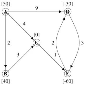
To further understand the concept of formulating a linear programming model from a a mini-mum cost flow network, an example will be given. For this example, a company with two factories (A and B), two warehouses (D and E), and one distribution center (C) will be looked at. This means that A and B are supply nodes, D and E are demand nodes, and C is a transshipment node. Also, given in the problem, the capacity on arc A→Bis 10 and the capacity on arcC→E is 80. All other arc capacities are unrestricted. The network formulated from this problem is show in Figure 2.1. The numbers labeling each arc represent costs and the numbers in brackets labeling each node represent supply and demand.

A B C D E [50] [40] [0] [-30] [-60] 2 4 9 3 1 3 2

From this network, the following linear programming problem was formulated. Note that the vectorxi j in the model below is in the formxi j= [xAB,xAC,xAD,xBC,xCE,xDE,xED]T

Minimize: z=2xAB+4xAC+9xAD+3xBC+xCE+3xDE+2xED Subject to: xAB +xAC +xAD =50 −xAB +xBC =40 −xAC −xBC +xCE =0 −xAD +xDE −xED =−30 −xCE −xDE +xED =−60 xAB≤10, xCE ≤80, and allxi j≥0

Using the simplex method mentioned in the previous section, this linear programming problem can be solved and an optimal solution can be found. The optimal objective value isz∗_{=490, where} the optimal values ofxi j are given in the matrixx∗= [0,40,10,40,80,0,20]T. z∗is the minimum

cost of shipping the product in supply in order to satisfy the demand. Eachxi j value represents the

amount of product being shipped from nodeito node j. Dual of the Minimum Cost Flow Problem

By putting the linear programming problem from above into standard form, explained in the pre-vious section, the dual can be found directly [6]. The dual of this problem is shown below.

Maximize: w=50y1+40y2−30y4−60y5−10y6−80y7 Subject to: y1 −y2 −y6 ≤2 y1 −y3 ≤4 y1 −y4 ≤9 y2 −y3 ≤3 y3 −y5 −y7 ≤1 y4 −y5 ≤3 −y4 +y5 ≤2

y₆,y7≥0

Solving this problem using the simplex method, the optimal value equals the value of the primal found above, meaning the solution found for the primal is, in fact, optimal. This is a result of the Strong Duality Theorem mentioned in the previous chapter [7].

The general form of the dual problem for the minimum cost flow problem is found below. Maximize: w= n

∑

∑

∑

yi−yj−vi j ≤ci j ∀ nodes iand arcs i→ j (2.12)

vi j ≥0 ∀ arcs i→ j (2.13)

yi unconstrained ∀ nodes i (2.14)

where the variablesyiandvi j are the decision variables. Eachyicorrespond to the flow constraints

and each vi j correspond to the capacity constraints.The dual found in the example above can be

derived using this model instead of the primal problem.

2.2.2

Assignment Problem

Another type of network flow problem is called the assignment problem. This problem deals with the assignment of people to different tasks [11]. The problem starts with a set S made up of m

people and a setD made up of mtasks. The cost associated with assigning personi to task j is given byci j. There is also a binary constraint on the decision variables.

xi j =

1 if personiassigned to task j

0 otherwise

The objective is to minimize the total cost in assigning every person to their different tasks. The objective function for the assignment problem is displayed below.

Minimize

∑

∑

There are also a few main constraints associated with the assignment problem. When assigning people to tasks, each person can only be given exactly one task. The constraint that each person is assigned to exactly one task is given by

∑

xi j =1, ∀i∈S. (2.16)

There is also the issue of making sure that each task is assigned a person, such that no task is left uncovered. The constraint that every task is assigned to exactly one person is given by

∑

xi j=1, ∀j∈D. (2.17)

The assignment problem can be solved similarly to the minimum cost flow problem.

2.2.3

Network Simplex Method

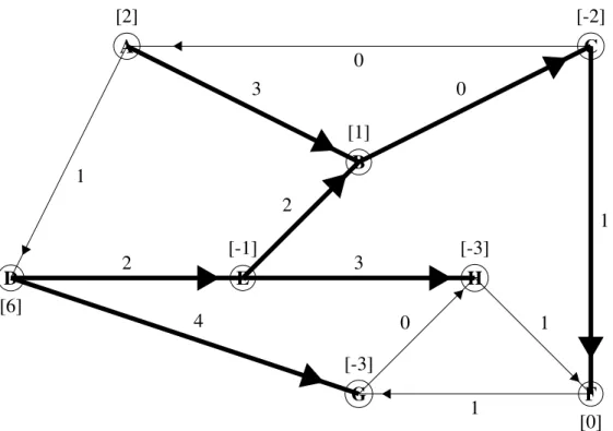
Both network flow problems mentioned in this section can be solved using the simplex method, which was briefly mentioned in the precious chapter, or by implementing the network simplex method. The network simplex method follows a similar algorithm as the simplex method: start with a basic feasible solution, choose an entering variable, choose a leaving variable, and solve for the new basic feasible solution. The difference comes in when conducting each iteration; the network structure of the problem is used instead of the simplex tableau. This expedites the run time of the algorithm. The following is an example of how to obtain the optimal solution of a minimum-cost network flow problem using the network simplex mehod. Shown below in Figure 2.2 is an initial network for such a problem [11].

In this network, the values associated with each arc are the cost values, ci j, and the values

associated with each node are the supply and demand values, bi j. bi j <0 signifies demand and

bi j >0 signifies supply. Whenbi j =0, as it is for node F, the node is a transshipment node, where

there is neither supply nor demand. The bold arcs in the network form what is called a spanning tree, which is a subset of the entire tree formed by all arcs in the network. One main quality of a spanning tree is for it to be connected and contain no cycles. Also, for a tree withmnodes,m₋1 arcs make up the spanning tree.The bold arcs also represent the basic variables in the solution and the remaining arcs represent the nonbasic variables.

Looking at the direction of the arcs in the spanning tree, as well as the supply/demand values on each node, the primal flow values on each arc can be calculated using the first constraint in the minimum cost flow problem, which was mentioned earlier in this section. The primal flow vari-ables determine if the network flow problem is primal feasible or not. If the primal flow varivari-ables are all non-negative, then the problem is primal feasible. If one or more primal flows are negative, then the problem is primal infeasible. The following equations are developed from this constraint in order to solve for the primal flows.

A B C D E F G H [2] [1] [-2] [6] [-1] [0] [-3] [-3] 0 3 0 1 2 1 1 0 4 2 3 1

Figure 2.2: Initial Network Solution - with cost and supply/demand values

Node A:xAB=2 Node B:xBC−xAB−xBE =1 Node C:xCF−xBC=−2 Node D:xDE+xDG=6 Node E:xBE+xEH−xDE =−1 Node F:−xCF =0 Node G:−xDG=−3 Node H:−xEH=−3

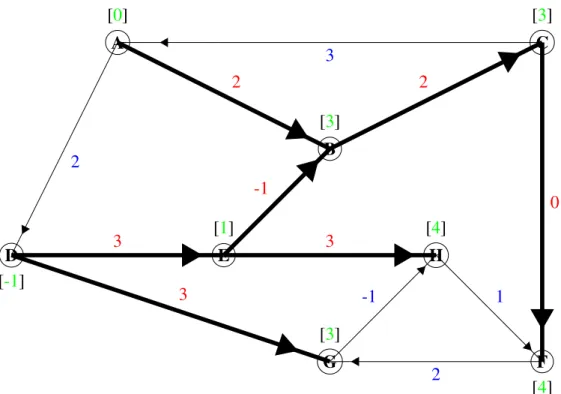
These primal flows are shown in red in the network in Figure 2.3. All flows associated with the nonbasic arcs are 0.

From here, the current objective value, z, for the primal problem can be calculated. This is done by taking the product of the cost and flow on each basic arc in the spanning tree,ci jxi j, and

summing all of the products.

z= (3∗2) + (1∗0) + (0∗1) + (3∗2) + (3∗3) + (4∗3) + (2∗ −1) =31

Next, by setting a root node, say yA, equal to zero, the dual variables can be calculated using

Arc (a,b):yb−ya=3 Arc (b,c):yc−yb=0 Arc (e,b):y_b−ye=2 Arc (d,e):ye−yd=2 Arc (e,h):yh−ye=3 Arc (c,f):yf−yc=1 Arc (d,g):yg−yd=4

These dual variables are shown in green in Figure 2.3.

The dual variables can be used to calculate the objective value, wfor the dual problem. This value is obtained by taking the product of the supply or demand and dual variable at each node,

biyi, and summing all the products.

w= (0∗2) + (3∗1) + (−2∗3) + (6∗ −1) + (−1∗1) + (0∗4) + (3∗ −3) + (−3∗4) =−31

The next step is to obtain the dual slack variables,zi j. These can be calculated for each

nonba-sic arc not in the spanning tree by using the equation zi j =yi−yj+ci j. The dual slack variables

determine if the network flow problem is dual feasible or not. If the dual slack variables are all non-negative, then the problem is dual feasible. If one or more dual slack variables are negative, then the problem is dual infeasible. We can calculate the dual slack variables as shown here: Arc (c,a):zca=yc−ya+cca=3−0+0=3

Arc (a,d):z_ad =ya−yd+cad =0−(−1) +1=2

Arc (f,g):zf g=yf−yg+cf g=4−3+1=2

Arc (h,f):zh f =yh−yf+ch f =4−4+1=1

Arc (g,h):z_gh=yg−yh+cgh=3−4+0=−1

These values for the dual slack variables are shown in blue in Figure 2.3.

Since the problem is both primal infeasible and dual infeasible, an iteration of the network simplex method must be carried out. First, choose the nonbasic arc with the most negative dual slack value as the entering arc. This will create a cycle within the network. Next, set the flow value for this arc tot. In the cycle, arcs traveling in the same direction as the entering arc will have an increase of flow by t and arcs traveling in the opposite direction will have a decrease of flow byt. Ast is increased, the arc with the flow reaching its lower or upper bound first will be cho-sen as the leaving arc. In this example, arcg_→his the entering arc and arcd_→eis the leaving arc. This process can be repeated until the objective value for the primal is equal to the objective value for the dual, and all primal flow values and dual slack values are nonnegative.

A B C D E F G H [0] [3] [3] [-1] [1] [4] [3] [4] 3 2 2 0 -1 1 2 -1 3 3 3 2

Chapter 3

Background: Course Scheduling

There are a variety of ways that course scheduling can be approached. Due to the complexity of the scheduling problem, it is useful to understand different methods of dealing with the scheduling problem that are approached at different universities.

3.1

Applications of Course Scheduling

An example of a more useful system of scheduling was one created to help Texas A&M Univer-sity [5]. The problem is to schedule faculty and subject assignments into rooms and times, which can be seen as a network optimization model with standard constraints. These constraints include requiring that all scheduled sections be staffed and having a maximum and minimum number of assignments for a faculty member. When assigning classrooms and times, there are also scheduling constraints including not assigning a faculty member more than one course per time period and not assigning more than one class for the same room and time period.

The method proposed is a network-based decision support system that has been used success-fully in improving the usage of classroom resources in addition to considering faculty preferences for subject, room, and time schedules. This new method was effective in dealing with a large, complex process that allowed the decision makers to maintain control of the process. Unlike past systems focused on the scheduling problem, this system simultaneously considers the dimensions of faculty, courses, classrooms, and time. There are several levels of nodes to be considered: mas-ter source, departmental, faculty/staff, room size/time level, and masmas-ter sink. The masmas-ter source and master sink nodes are used to circularize the network. These are the five classes of nodes or constraints in this network model. All of these factors contribute to how this system is set up and what the constraints will have to be. Room sizes and time levels are grouped together in this model such that they are classified as one level of node. This means that each room size at each time slot is its own node, so room size and time are not assigned separately.

use all of their resources in the most efficient way. This was, in part, due to the fact that each department was given priority over certain classrooms in which they could schedule any of their sections, as long as they were smaller than 75 percent of the classroom seating capacity. For much of the remaining unscheduled class sections and unused room and time slots, courses were as-signed during a group bargaining session.

The proposed model is a capacitated network flow problem with an objective function set up to include a penalty structure. Upper bounds include the room size as well as the number of rooms. There are also only a certain number of classes that each faculty member is able to teach. Time slots can vary for different classes, but it is important to minimize all conflicts as much as possible. The network model has an objective function that sets to minimize the total number of arcs for the faculty and class sections assigned to room/time pairs. The constraints include conflict avoid-ance constraints, which are given by the following equation.

∑

∑

XA(i,j,s,t)_≤1 _∀i,j (3.1) where(i,j)represents a faculty and subject node,srepresents a room size,trepresents a time, and

XA(i,j,s,t)is the arc connecting them.These constraints act to eliminate any conflicts that could

come up in scheduling, including preventing faculty being assigned multiple classes to the same room at the same time. Realistically, the model would only include those arcs that represent the assignment to rooms with sufficient capacity and do not violate size restrictions.

The model is initially solved without conflict avoidance constraints XA(i,j,s,t), since there is

no guarantee that constraints of this form must be imposed in order to generate a feasible solution. If the resulting solution does not contain any conflicts, then the problem is finished. If there are conflicts that require these constraints, then the generated solution is used as an advanced starting point for the constrained problem. The two processes for going through this problem are a manual process and an automated process. The manual process involves the department head preparing a preliminary schedule and then the departments meeting with unassigned rooms and courses and attempting to assign the maximum possible, giving the best manual solution. Finally, a list of any other unassigned rooms and courses is sent to the university for scheduling. The automated process involves solving the model and checking for any infeasibility based on the course and time preferences submitted to the Dean’s Office, resulting in the best network solution. The results are then returned to the department for review and any further alteration in assignments. Using this process, the schedules will tend to stay the same from year to year once the database for a particular setting is created. So instead of re-creating the database, it can be modified to reflect current needs and preferences.

3.1.1

Course Timetabling

Course timetabling is another word for course scheduling. A timetable consists of a set of meet-ings that each have a start and end time. Other information can be associated with these meetmeet-ings, such as a room or the number of people attending [2]. When dealing with course scheduling, a timetable containing each course, and its associated information, can be created. A standard course timetabling problem consists of several different sets that are associated with a course. Different scheduling problems use different sets and information to solve the problem. More specifically, course timetabling can be seen as an assignment problem consisting of various resources. In the course timetabling problem, courses are assigned to a set of available classrooms and start times. Depending on the type of class being assigned, the end times can vary. Timetabling is mainly used by higher-level institutions and universities for assigning courses to rooms and times, or assigning students and faculty to courses [3].

The main set of a timetable is a set of courses. This set contains each course with an associated number of hours the course is held during a week. Each course is then divided into sections. Some courses may only have one section, but others may have several sections. This usually depends on the number of students needing, or wanting, to take the course. Sections of the same course may also not be held in the same room and/or at the same time. Each section is then associated with lessons, which can be lectures, conferences, or labs. These lessons can have different duration times, as well as held in different rooms and/or at different times. These classes are designed by the schedule planners, in accordance with the structure of degrees and past experience with stu-dents’ choices. The timetable also consists of a set of teachers and a set of rooms, both with fixed capacities. Teachers are previously assigned to sections, and rooms are of different types, such as lecture halls and computer labs. Lastly, a week is defined, which is made up of a set of periods, or times. Each day of the week has the same number of periods associated with it. A timetable is also able to contain preassigned courses or periods, where the rooms, times, and other information cannot be changed for certain courses.

In order to schedule the courses in the most efficient way, constraints are added to the problem. Each course timetabling problem has a set of hard constraints and a set of soft constraints that it must satisfy. The hard constraints can include:

• Every course must be assigned to a room and time.

• No professor can teach more than one course at the same time. • No room can be assigned to more than one course at the same time.

• The room assigned to a given course must be of the required type (i.e., a lab course requires

a lab room).

Soft constraints are not as important to satisfy as hard constraints. These constraints are helpful in improving the timetable but not absolutely necessary. Generally, the more the soft constraints

are satisfied, the better the timetable will be. They often contain constraints on faculty or student preferences, or a constraint that limits the lessons of a class assigned to a minimum number of different rooms.

The solution procedure for solving a course timetabling problem can be broken down into three main steps: construct an initial timetable, improve that timetable, and improve the room assignment [1]. In the first step, an initial timetable is constructed by assigning each course section to both a room and time. In some cases, an initial timetable is given. Thus, to start, let x∗ _{be a} feasible solution. The second step involves using an algorithm to solve the optimization problem and improve the initial timetable. One such algorithm is known as the Tabu Search procedure. The Tabu Search involves swapping classes in order to improve the objective function value. In the last step, the room assignments are changed in order to improve the timetable and the time assignments are fixed. This is different from the previous step where both the room and time assignments were not fixed.

Applications of Timetabling

Purdue University’s system of scheduling is a good example of how course timetabling can be used [9]. Currently course schedules are developed at Purdue University using a decentralized process. To be decentralized means that departments can respond to demand changes, instructor availabil-ity and other factors while the Space Management and Academic Scheduling (SMAS) Department schedules most course offerings in classrooms allocated to them, where each department has its own set of criteria for assigning instructors to sections and sections to rooms and times. Instructor preferences are considered based on room capacity and other constraints.

A schedule is built for each semester at Purdue, and determining course demand and classroom requirements is the first step before the schedule is built. The process then consists of requesting large lecture rooms, building a master course schedule, and assigning students to sections. While the decentralization scheduling process has worked fairly well for Purdue, it produces schedules that could be potentially be improved given better information and faster scheduling methods.

The program used in this case is a minimax problem in which the goals are to both minimize the maximum expected common enrollment between two sections scheduled at the same time and maximize instructor time preferences, room fit and paired section and slot preferences. There are set-packing constraints that restrict room and instructor assignments to available capacity. The constraints also include instructor and room conflict constraints, but these are only valid if time patterns do not overlap. The room conflict constraint is such that no more than one course section can be assigned to each classroom/time combination. Another constraint that the Purdue classroom scheduling model uses is a multiple-choice constraint that requires a slot assignment for each section. The final constraint of the minimax model restricts room assignments to those that meet or exceed section capacity as well as restricting time pattern choices to those that match meeting time requirements for each section.

Chapter 4

Project Formulation

The goal of this project is to develop a mathematical model and a software tool that will help WPI develop a more efficient schedule. For this project, efficiency is defined as the ratio between the population limit of a course to the capacity of a classroom. The efficiency of assigning courseito room jis defined as

Course Population(i)

Room Capacity(j)

where a course refers to a meeting (lecture, conference, or lab) of a section of a course and a room refers to any schedulable room, or space, on campus. The total efficiency of a schedule is defined as

∑

∑

Course Population(i)

Room Capacity(j) Hi j

whereHi j will be called the happiness coefficient. This coefficient is a weight placed on the

effi-ciency, giving a penalty or reward for assigning courseito room j. It is defined as

Hi j =

  

0 if room jis a bad pair for coursei

1 no preference

1.5 if room jis a preferred pair for coursei

An assignment is considered inefficient if Course PopulationRoom Capacity. If Course Population> Room Capacity, the efficiency is defined to be zero. This will be explained further in section 4.4.

In order to understand the problem, the team first explored the global scheduling problem and formulated the linear programming model associated with it. This was then simplified to the model

for the local scheduling problem. Lastly, the local linear programs were optimized using Matlab and a new, and improved, schedule was created. These steps will be outlined in more detail in the following sections of this chapter.

4.1

Global Scheduling Problem

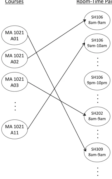
To begin understanding the global scheduling problem, the team first visualized a schedule in network form. After much deliberation, the network in Figure 4.1 was produced. This displays the current schedule for Calculus I at WPI. Notice, this is similar to the assignment problem mentioned in Chapter (insert network flow chapter here).

!"#$%&$# "%$# !"#$%&$# "%&# !"#$%&$# "%'# !"#$%&$# "$$# ()$%*# +,-./,-# ()$%*# /,-.$%,-# ()$%*# /0-.$%0-#

1#1#1#

1#1#1#

1#1#1#

1#1#1#

1#1#1#

Figure 4.1: Schedule for Calculus I (only lectures)

labs would be represented by separate nodes. The nodes on the right represent room-time pairs. A room-time pair, in this case, is made up of a classroom, time, schedule type, and duration time, where schedule type refers to the set of days the course is held on. An arc between a course node and a room-time pair node represents an assignment between that course and room-time pair.

Since there are a greater amount of room-time pairs than there are courses, a number of dummy courses were created, one for each room-time pair not already assigned to a course. These dummy courses are treated as any other course in the schedule and they have a course population of 0. The room-time pairs associated with a course in the schedule are called occupied and the room-time pairs associated with a dummy course are called available.

The total number of courses and dummy courses in a full schedule are given by NC and the

number of room-time pairs are given byNRNT. An assignment between a course and a room-time

pair will be determined by the value of the decision variable,xi j. This variable will be equal to 1

when courseiis assigned to room-time pair jand 0 otherwise.

From this network, a binary integer program was formulated. This is shown in Equations 4.1-4.3 below. The last constraint shown is the binary constraint.

Maximize NC

∑

∑

∑

∑

1 if courseiassigned to room-time pair j

0 otherwise

The objective of this problem, shown in Equation 4.1, is to maximize the efficiency of the schedule as a whole. The first constraint, Equation 4.2, says that for every course, or dummy course, in the schedule, there is exactly one room-time pair assigned to it. The second constraint, Equation 4.3, says that for every room-time pair, there is exactly one course, or dummy course, assigned to it. These restrict (i) a course from being held in more than one room during one time and (ii) more than one course from being held in the same room during the same time. This global problem is known as an NP-hard problem, which defines the complexity of the problem. NP-hard suggests that there is no known algorithm to solve this problem in a feasible amount of time.

4.2

Local Scheduling Problem

Due to time constraints and the complexity of the global problem, it was simplified into smaller subproblems, which will be called local scheduling problems. Before defining what a local prob-lem is for project, a block must be explained. A block is defined as a set of courses with the same schedule type, start time, and duration time. Examples of blocks are the set of courses held on MTRF at 9:00am for one hour or the set of courses held on MR at 12:00pm for two hours. In total, there are 21 schedule types, 14 start times, and five duration times included in the current schedule at WPI, which totals to a possible 1,470 blocks.

Each block is associated with a local linear program, whose objective is to maximize the effi-ciency of a subset of a schedule, or block. The linear program associated with blockk is shown below. Maximize N_Ck

∑

∑

∑

∑

1 if courseiassigned to room-time pair j

0 otherwise

whereNCk is the number of courses, and dummy courses, in blockkandNRkNTk is the number of

room-time pairs associated with the courses and dummy courses in blockk. Because each block consists of only one start time, NTk =1. The objective of the local problem is to maximize the

efficiency of a block. The sum of all local efficiencies is less than or equal to the total global effi-ciency, where local efficiencykis defined to be the total efficiency of blockk.

As one may notice, the global linear program and the local linear program are very similar; the local problem is a more constrained version of the global problem. The sets of courses and room-time pairs associated with each block are subsets of the sets of total courses and room-time pairs associated with the entire schedule in the global problem.

4.3

Data Processing

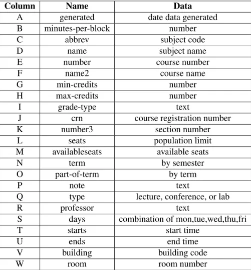
3,118 rows, each representing a course section meeting, and 23 columns, each representing differ-ent information about the meeting. The rows are first ordered alphabetically by subject code, then course number, section number, and term offered, and finally by meeting type. The different types of columns are listed in Table 4.1 below. The data that the team is mainly concerned with is seats, part-of-term, type, days, starts, ends, building, and room.

Column Name Data

A generated date data generated

B minutes-per-block number

C abbrev subject code

D name subject name

E number course number

F name2 course name

G min-credits number

H max-credits number

I grade-type text

J crn course registration number

K number3 section number

L seats population limit

M availableseats available seats

N term by semester

O part-of-term by term

P note text

Q type lecture, conference, or lab

R professor text

S days combination of mon,tue,wed,thu,fri

T starts start time

U ends end time

V building building code

W room room number

Table 4.1: Column Data From Excel Spreadsheet

This data was then preprocessed within Excel in order to expedite the run time in Matlab during optimization. The first step was to reformat the raw data that was given. In Excel, the start and end times were given in the form 8:00AM, which Matlab does not recognize as a time. Therefore, a space was inserted and this was replaced by 8:00 AM. Two new columns were then created, start hour and end hour. For each start time, the hour is placed in the start hour column. For each end time, the hour plus one is placed in the end hour column. Next, the days column was copied and separated by commas into five columns using the text to columns function in Excel. These five new columns are called day1, day2, day3, day4, and day5. Five additional columns were added

called timeday1, timeday2, timeday3, timeday4, and timeday5. These columns were created by concatenating the corresponding day columns with the start hour column. These columns represent the time-day pairs for each course section meeting. Lastly, the building and room columns were concatenated, creating the room combo column.

After this reformatting was complete, the team placed indices on all building-room combina-tions, schedule types, times, and time-day combinations. The ordering for each can be found in the lookup tables Appendix B. All indices start at 1, except for the time indices; these start at 0. Index columns were then added after the schedule type, timeday1-timeday5, start hour, end hour, and room combo columns. The full set of steps for reformatting the data is outlined in Appendix A.

4.4

Optimization

Once the problem was formulated and the data was preprocessed, the team was able to use a built-in function in Matlab called bintprog, a binary integer programming function for linear optimization, to optimize the local linear programs. In order to begin optimizing the efficiency of the schedule, some initial set-up was required. The first step was to define variables, such as the lists of total rooms, times, days, schedule types, and room capacities. The rest of the necessary information used was taken directly from the columns in the Excel spreadhseet. Values are then given to the happiness coefficients for each course-room pair using the values mentioned earlier in this chapter. The following three sections explain the other necessary steps taken in Matlab in order to improve the current schedule.

4.4.1

Occupation Matrix

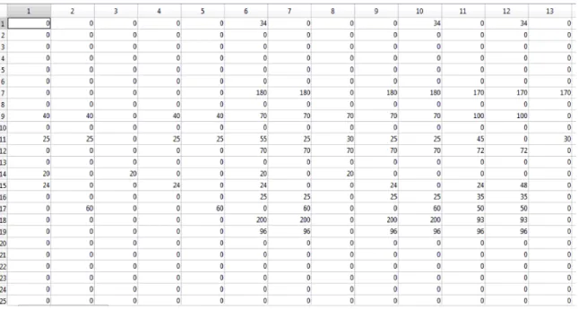
Using the preprocessed data from Section 4.3, a matrix, called the occupation matrix, was devel-oped. There are several representations of the occupation matrix, all of which are used during optimization. Each one begins as a zero matrix, or a matrix with all entries equal to zero. For all representations, the rows represent a schedulable room and the columns represent time-day pairs. The ordering of the rows corresponds to the ordering of the room vector. The columns are ordered such that the days cycle through within each time, i.e. Monday 8am, Tuesday 8am, ..., Friday 8am, Monday 9am, ..., Friday 10pm.There are a total of 5 days×14 times = 70 time-day pairs in the current schedule.

The first representation of the occupation matrix displays the number of sections held in each room during any time-day pair. This will be called the main occupation matrix. This matrix was created by adding a 1, representing a single section meeting, to each entry that corresponded to a room occupied during a time-day pair. This occupation matrix can be found in Figure 4.2. For the purposes of optimization, another matrix was created by taking the minimum of these entries and 1. This produced a matrix of all 0s and 1s, where 1 corresponds to there being at least one section

in a room during a time-day pair and 0 if the room is available.

Figure 4.2: Occupation Matrix Displaying Number of Sections

The second representation will be called the occupation-population matrix. This matrix dis-plays the population limit of students occupying each room during any time-day pair. This matrix was created in a similar way as the main occupation matrix, where the population limit of each course was added to the entries in the matrix. This occupation matrix can be found in Figure 4.3.

The third representation is called the occupation-efficiency matrix, which displays the effi-ciency levels of each room during any time-day pair. This was found using the occupation-population matrix and dividing them by the corresponding room capacities of each room. This occupation matrix can be found in Figure 4.4.

The final representation is a set of sub-occupation matrices, one for each block. These matrices display the minimum number of sections held in a room during any time-day pair for the schedule type, start time, and duration time associated with the block. The rest of the entries in the matrix are 0.

The most useful representation, outside of optimization, is the occupation-efficiency matrix. This creates a visual representation of how efficiently each room is being used during any time within the week. It also displays the available rooms, which are represented by a 0 efficiency level.

Figure 4.3: Occupation Matrix Displaying Course Populations

Figure 4.4: Occupation Matrix Displaying Efficiencies

4.4.2

Model

The next step was to code the linear program from Section 4.2 into Matlab. To do this, the variables th

sub-occupation matrix, the entries in each row are summed. If the sum for row j is greater than 0, room jis occupied during the start time and days of the week specified by block k. Using the minimum of the main occupation matrix, the entries in each row are also summed. If the sum for row j equals 0, room j is available at all times during the week. NRk is defined to be the total

number of occupied and available rooms for blockk. NCk is found by searching through the Excel

Spreadsheet and finding the courses in blockk. Each constraint of the local liner program is then coded into Matlab using these variables.

From there, the efficiencies for each course-room pair were defined. This is done using the ef-ficiency definition in Equation 4.4 from Section 4.2. It is actually possible that, in the given initial schedule, that a course meets in a room with a capacity that is lower than the population limit of the class. In such a case, the efficiency of the assignment is greater than 1. This situation should be avoided. In this implementation, all efficiencies over 100% are replaced with 0. This gives the same effect as setting the happiness coefficient to 0 in such a case; that is, issuing a penalty. The advantage of this approach is that, by relaxing the hard constraint on the upper bound of efficiency, there is no need to add constraints to the model. Adding this amount of constraints could poten-tially cause the program to crash.

Using all of the information outlined in this section and the one previous, the Matlab function bintprog was implemented. This function uses the branch and bound algorithm in order to find an optimal solution. The local linear programs are optimized in sequence, each optimization giving the optimal solution for that block. In the situation of zero courses contained in a block, this block is skipped during optimization.

The order of optimization is defined by three consecutive ’for’ loops, one for each schedule type, start time, and duration time. The order currently imposed in Matlab is schedule type, start time, then duration time. The final solution does depend on this ordering, however, the effects of a different ordering are currently unknown.

4.4.3

Update

After optimizing a local linear program, courses may move from one room to another. If a course does move, the room it was previously assigned to becomes available and the room that it moved to becomes occupied. Because of this change, the occupation matrices must be updated after each optimization. This is done by comparing the initial solution to the final solution for the block.

After one full cycle of optimizing all local linear programs once is complete, the final solution is the new, and improved schedule. This improvement can be seen through the final total efficiency, which is the sum of all efficiencies from each optimization. Because the local linear programs are being solved in sequence and courses are constrained from moving between blocks, there may be a better solution than the one produced due to the occupation matrix updating after each step. This also means that the final total efficiency produced may not be equal to the final total efficiency of

the global problem. In order to improve the efficiency further, several cycles can be optimized in sequence.

4.5

Adding a New Course

While switching classroom assignments for courses is an important aspect of this project, it is not the only process that should be considered. In the event of adding a new class to a schedule, appropriate steps must be taken. The team has created an algorithm that, given the necessary information for a new course, places this course into the best possible room. The algorithm is as follows.

1. Given the limit, schedule type, start time, and duration time of the course being added, determine the block containing this course.

2. Input the new course’s student population limit.

3. If feasible rooms available in block, compute efficiencies of assigning new course to these available rooms.

(a) Find room with maximum efficiency. (b) Assign new course to this room.

STOP

Else compute efficiencies of assigning new course to feasible rooms occupied in block. (a) Find room with maximum efficiency.

(b) Assign new course to this room. Course previously assigned to room is removed and becomes the ’new course’ to be added to the schedule.

(c) Go to Step 2.

A feasible room, in this case, is defined as a room whose capacity is less than or equal to the population limit of the course being added. The algorithm is repeated until the new course being added to the schedule is assigned to an available classroom.

Chapter 5

Results and Analysis

After implementing the model in Matlab, we were able to determine the change in efficiencies from the initial schedule to the new generated schedule. This was done by first comparing the initial efficiencies of each individual block to the final efficiencies of each, and then by comparing the initial total efficiency to the final total efficiency of the entire schedule after one optimization cycle. For this, all happiness coefficients are set to 1 for simplicity.

The initial total efficiency of the current schedule was 259.252. Looking at only lectures in the A-term schedule, there are a total of 572 course section meetings. This means that, on average, 45.32% of classroom space was utilized during any time. After optimization, the team obtained the final total efficiency of 322.663, which averages to about 56.41% of classroom space used. This gives an 11.09% efficiency increase between the current schedule and the improved schedule. That is just after one cycle of optimization. Repeating this procedure, the total efficiency level continues to increase.

The local efficiencies of each block are subject to change depending on the order in which the local problems are optimized. The first block to be optimized with one ordering may not be first to be optimized with another ordering. It should be noted that the improved schedule obtained during this project is just one of several possible feasible solutions. The effects of another ordering are currently unknown.

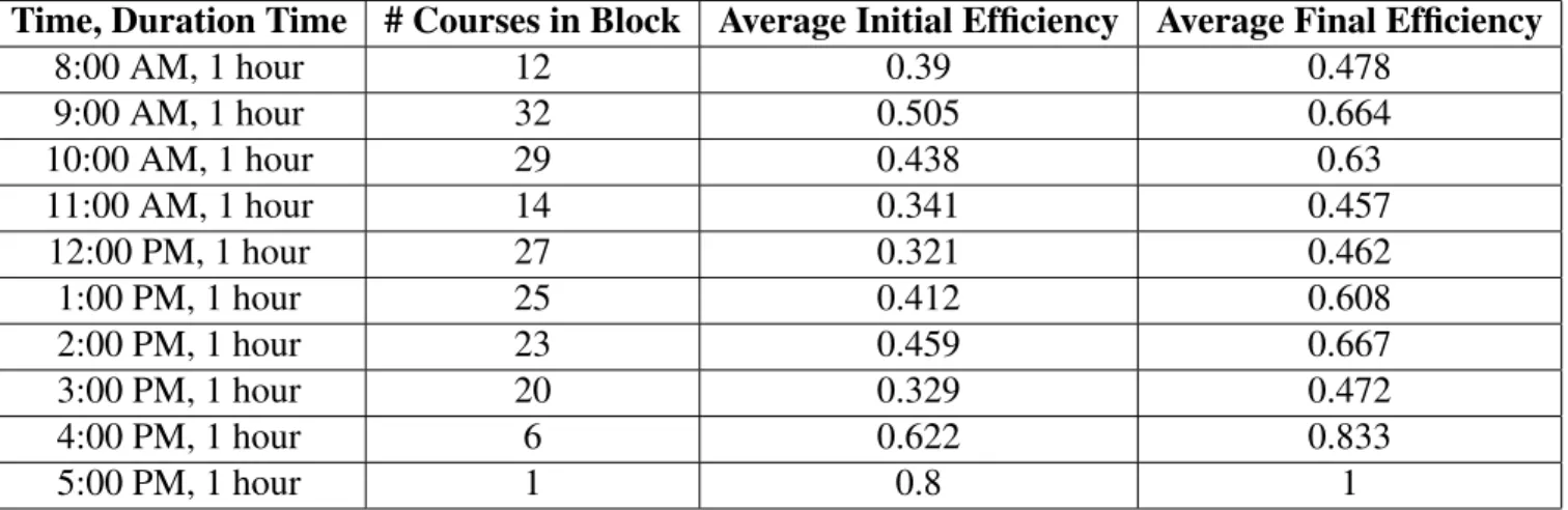
To investigate the effects of optimizing each block separately have on the final total efficiency of the schedule, the team compared the efficiencies of each block after optimization. Table 5.1 below shows the changes in efficiencies for all blocks associated with the MTRF schedule type.

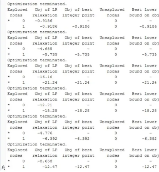
The information provided in the table can be extracted from the output in Matlab after opti-mization. A sample of this output is shown in Figure 5.1. Other information, such as the number of iterations taken to optimize each block, can also be extracted from the output in Matlab. This can be seen in Figure 5.2.

effi-Time, Duration Time # Courses in Block Average Initial Efficiency Average Final Efficiency 8:00 AM, 1 hour 12 0.39 0.478 9:00 AM, 1 hour 32 0.505 0.664 10:00 AM, 1 hour 29 0.438 0.63 11:00 AM, 1 hour 14 0.341 0.457 12:00 PM, 1 hour 27 0.321 0.462 1:00 PM, 1 hour 25 0.412 0.608 2:00 PM, 1 hour 23 0.459 0.667 3:00 PM, 1 hour 20 0.329 0.472 4:00 PM, 1 hour 6 0.622 0.833 5:00 PM, 1 hour 1 0.8 1

Table 5.1: Changes in Efficiency for MTRF Schedule Type Blocks

ciencies and the average final efficiencies for each block. This increase is seen after optimizing every block in the model. Thus, the increase in total efficiency of the schedule is not surprising at all. One thought to keep in mind is the schedule that is produced from this is an improvement on the current schedule, not the optimal schedule.

Figure 5.1: Efficiency Output From Matlab

Chapter 6

Conclusions

The challenge with the current course scheduling system at WPI is incorporating all restrictions and preferences for classrooms and times in an easy manner, as well as changing the course schedule as needed. The schedules produced are not always as efficient as they could be, which lowers the total efficiency of the entire schedule. This project created a software tool that:

• automates part of the course scheduling process;

• improves the efficiency of the current schedule by changing classroom assignment of courses with the same schedule type;

• reads course schedule information exported directly from Banner;

• produces an occupation matrix displaying the efficiencies of every room during any time and day.

The team introduced the use of the happiness coefficients which are weights on the efficiencies. These weights give a penalty or reward for certain course-room assignments. This can be used to reflect faculty preferences and constraints on courses being held in certain rooms, i.e. chemistry lab courses must be held in a chemistry laboratory.

One additional challenge was to create an automated system to add a new course to a given schedule. The team created an algorithm to do this. By looking at available rooms first, and then occupied rooms, the algorithm places a new course into the most efficient room, with a specific schedule type, start time, duration time, and student population of the new course.

The most challenging aspect of this project was the formulation of the linear programming model. The model created by the team is one of several possible formulations that may be used to produce a feasible solution. Starting with the global scheduling problem, the team simplified it in order to create the local linear programming model. Even though the program that was created does not find an optimal schedule for the global problem, it does improve the current course schedule using the local problems and can be used as a basis for a more general schedule optimizer.

6.1

Recommendations

The first recommendation that the team would like to make is to expand the definition of a block to allow a larger class of available swaps and to improve global efficiency. Currently, a block restricts courses to having the same schedule type, start time, and duration time in order to switch between room assignments. That is, two courses with different schedule types would not be allowed to switch rooms in the current model, even if the switch would cause the efficiency of the schedule to increase. Allowing switches between blocks would be beneficial. An even more interesting switch would be to switch multiple room assignments at once. For example, a two-hour long course held at 9am on Monday and Thursday and another one held on Tuesday and Friday can potentially switch with two one-hour long courses on Monday, Tuesday, Thursday, and Friday at 9am and 10am. Expanding the definition of a block and making these switches possible could prove to be beneficial to increasing the efficiency of the entire schedule.

The team would also recommend the creation of a user interface that would allow for the au-tomation of the entire improvement process. This would allow the user to easily, and automatically, export data from Banner, upload it into Matlab, run the optimization, produce an improved sched-ule, and upload this new schedule directly into Banner, just with the touch of a button. A way to undo an assignment or see changes as they are made would also be beneficial. There is also an option to create an automated system for department heads to update the happiness coefficients according to preferences within their respective departments.

Additional recommendations for future projects are listed below.

• Define constraints on the upper bound of efficiency (currently set at 100%), as opposed to

incorporating it in the objective function.

• Perform sensitivity analysis on the happiness coefficients to investigate how changes in the

values affect the solution.

• Use negative values, rather than 0, as the penalty for exceeding 100% efficiency.

• Validate the improvements made to the schedule by looking at the dual problem. • Experiment with other software (CPLEX) or using a C library within Matlab. • Create macro in Excel following the steps outlined in Appendix A.

The team hopes that all of these results and conclusions obtained during this project will pro-vide a starting point to future project teams in order to propro-vide WPI with a more efficient course schedule. In addition, the team hopes these results will aid WPI to begin the process of improving their course scheduling system, and the efficiency of the course schedule overall.

Bibliography

[1] Alvarez-Valdes, Ramon, Crespo, Enric, Tamarit, Jose M. Design and Implementation of a course scheduling system using Tabu Search, European Journal of Operational Research 137 (2002) 512-523.

[2] Burke, Edmund, Jackson, Kirk, Kingston, Jeffrey H., and Rupert Weare. Automated Uni-versity Timetabling: The State of the Art, The Computer Journal, Vol. 40, No. 9, 1997. [3] Carter, Michael W., Laporte, Gilbert. Recent Developments in Course Timetabling,

Lec-ture Notes in Computer Science, 1998, Volume 1408/1998, 3-19, University of Toronto, Department of Mechanical and Industrial Engineering.

[4] Denardo, Eric V. Linear Programming and Generalizations. Springer: New York, New York, 2011.

[5] Dinkel, John J., Mote, John, Venkataramanan. An Efficient Decision Support System for Academic Course Scheduling. Operations Research: Vol. 37, No. 6, Operations Research Society of America, 1989.

[6] G.L. Nemhauser, A.H.G. Rinnooy Kan, M.J. Todd, Handbooks in Operations Research and Management Science, Elsevier Science Publishers B.V. Netherlands, 1989.

[7] Hillier, Frederick S., Lieberman, Gerald J. Introduction to Operations Research, McGraw-Hill, New York, New York, 2010.

[8] Kornik, Chuck, Administrator of Academic Programs. Annual Report - 2010/11, Admin-istration of Academic Programs.

[9] Mooney, Edward L, Parmenter, W.J., and Rardin, Ronald L. Large-Scale Classroom Scheduling, IIE Transactions, 28.5, May 1996, p. 369.

[10] Schrijver, A. Theory of Linear and Integer Programming. Chichester: Wiley, 1986.

[11] Vanderbei, Robert J. Linear Programming: Foundations and Extensions, Springer: New York, New York, 2001.

[12] Worcester Polytechnic Institute, Division of Enrollment Management, 2011 Fact Book: Undergraduate and Graduate Student Enrollment Information October 1, 2011.

[13] Worcester Polytechnic Institute, Division of Enrollment Management, 2010 Fact Book: Undergraduate and Graduate Student Enrollment Information October 1, 2010.

Chapter 7

Appendix A: Steps for Reformatting Data in

Excel

Step 1: Open schedule data generate from Banner. Call this sheet ’Data’.

Step 2: Create five new sheets in the workbook. Call these sheets: Lookup Tables, A Term, B Term, C Term, D Term.

Step 3: Insert 16 columns to right of ’days’ column. Call these columns: schedule index, day1, day2, day3, day4, day5, timeday1, timeday1 index, timeday2, timeday2 index, time-day3, timeday3 index, timeday4, timeday4 index, timeday5, timeday5 index. Also, rename ’days’ column as ’schedule’

Step 4: Insert 2 columns to right of ’starts’ column. Call these columns: start hour, start index.

Step 5: Insert 2 columns to right of ’ends’ columns. Call these columns: end hour, end index.

Step 6: Insert 2 columns to right of ’room’ column. Call these columns: room combo, room combo index.

Step 7: Convert data in table to range data. Make sure first entry in each column is set to Number or General data. None should be Text data.

Step 8: Highlight ’starts’ and ’ends’ columns and Find & Replace all ’AM’ with ’ AM’ and all ’PM’ with ’ AM’. Format Cells to be category Time and type ’13:30’.

Step 9: Copy all entries of ’schedule’ column and paste into ’day1’ column. Use Text to Columns to separate text by commas into each ’day’ column.

Step 10: In first entry of ’timeday1’ column, type =AK2&U2 and copy this down to all entries in column. Reapeat for all ’timeday’ columns using corresponding ’day’ columns as

Step 11: In first entry of ’start hour’ column, type =HOUR(AJ2) and copy this down to all entries in column. In first entry of ’start hour’ column, type =HOUR(AM2)+1 and copy this down to all entries in column.

Step 12: In first entry of ’room combo’ column, type =AP2&AQ2 and copy this down to all entries in column.

Step 13: In first entry of ’schedule index’ column, type =VLOOKUP(Z2,’Lookup Tables’!$A$4:$B$24,2,FALSE) and copy this down to all entries in column.

Step 14: In fi