Quantum Error Detection by Stabiliser Measurements in a Logical Qubit

Quantum Error Detection by

Stabiliser Measurements in a

Logical Qubit

THESIS

submitted in partial fulfillment of the requirements for the degree of

MASTER OF SCIENCE in

EXPERIMENTALPHYSICS

Author : Mengzi Huang

Student ID : 1411004

Supervisor : Leonardo DiCarlo

2ndcorrector : Michiel de Dood

Quantum Error Detection by

Stabiliser Measurements in a

Logical Qubit

Mengzi Huang

黄

黄

黄

梦

梦

梦梓

梓

梓

Huygens-Kamerlingh Onnes Laboratorium, Universiteit Leiden P.O. Box 9500, 2300 RA Leiden, The Netherlands

PROJECT UNDERTAKEN AT

Quantum Transport Group Kavli Institute of Nanoscience Delft University of Technology

Lorentzweg 1, 2628 CJ Delft, The Netherlands

SUPERVISED BY

Dr. Stefano Poletto Dr. Leonardo DiCarlo

Abstract

Contents

List of Figures . . . vii

1 Introduction . . . . 1

1.1 Basic concepts of quantum information processing . . . 1

1.2 Quantum error and error correction . . . 4

1.3 Physical implementations . . . 7

1.4 Thesis objectives and overview . . . 8

2 Circuit QED with superconducting qubits . . . . 11

2.1 The transmon qubit . . . 11

2.1.1 From Cooper-pair box to transmon . . . 11

2.1.2 Frequency tunability and flux biasing . . . 13

2.2 Circuit quantum electrodynamics . . . 14

2.2.1 Cavity-qubit interaction . . . 15

2.2.2 Qubit readout and number splitting . . . 16

2.2.3 Qubit drive and single-qubit gates . . . 17

2.2.4 Multiple-qubit gates . . . 19

3 Experimental Methods . . . . 23

3.1 Device and setup . . . 23

3.1.1 The five-qubit processor . . . 23

3.1.2 Electronics and cryogenics . . . 24

3.2 Characterisations of quantum elements . . . 26

3.2.1 Readout and initialisation . . . 26

3.2.2 Coherence times . . . 27

3.3 Gate tuning . . . 30

3.3.1 Single-qubit rotation . . . 30

3.3.2 The iSWAP gate . . . 32

3.3.3 The CPHASE gate . . . 34

3.3.4 Phase errors induced by Stark effect . . . 36

4 Experiments and Results . . . . 43

4.1 Double-parity measurement . . . 43

4.1.1 Procedures and tune-ups . . . 43

4.1.2 Assessment . . . 45

4.2 Entanglement generation by stabiliser measurements . . . . 46

4.2.1 Single-qubit phase calibration . . . 46

4.2.2 Bipartite entanglement . . . 48

4.2.3 Tripartite entanglement and encoding a logical qubit 49 4.3 Quantum bit-flip error detection protocol . . . 53

4.3.1 Encoding by unitary gates . . . 53

4.3.2 Adding coherent errors . . . 56

4.3.3 Single-qubit phase calibrations . . . 56

4.3.4 Metrics and characterisation . . . 58

4.3.5 Incoherent errors and discrete assessments . . . 65

4.4 Phase-flip error detection . . . 66

5 Conclusions and Future work . . . . 69

5.1 Fast feedback with FPGA . . . 69

5.2 Towards universal and scalable QEC . . . 70

5.3 Conclusions . . . 71

References . . . . 73

List of Figures

1.1 Bloch sphere representation of a quantum bit . . . 2

1.2 The classical repetition code . . . 5

1.3 Schematics of three-qubit repetition code for bit-flip errors . 6 2.1 Circuit representation of a Cooper pair box . . . 12

2.2 Gate-charge dispersion of the eigenenergies of charge qubits 13 2.3 Schematic and example of circuit QED . . . 15

3.1 Photograph of the quantum processor . . . 24

3.2 Wiring diagram of the experimental setup . . . 25

3.3 Measurements of the coherence times of qubits and buses . . 28

3.4 Low-crosstalk simultaneous qubit readouts . . . 30

3.5 Fine tuning of pulse amplitude . . . 31

3.6 Tune-up of iSWAP gates . . . 33

3.7 Vacuum Rabi oscillations betweenDmand the buses . . . 34

3.8 Tune-up of CPHASE gates . . . 36

3.9 Calibration of phase errors induced by Stark effect . . . 37

4.1 Sequence of tuning double-parity measurement . . . 44

4.2 Typical results of double-parity tune-ups . . . 44

4.3 Characterisation of stabiliser measurements . . . 47

4.4 Witnessing two-qubit entanglement by stabiliser measure-ments . . . 49

4.5 Witnessing three-qubit entanglement by stabiliser measure-ments . . . 50

4.6 Tomographic verification of generating GHZ-type entangle-ment from a maximal superposition . . . 51

4.7 Encoding by stabiliser measurements . . . 52

4.8 CPHASE gates for the encoding step . . . 54

4.9 State tomography of encoding by unitary gates . . . 55

4.10 Complete sequence for the characterisation of quantum er-ror detection . . . 57

4.12 Characterisation of bit-flip error detection . . . 61 4.13 Three-qubit and logical fidelities under coherent bit-flip

er-rors for the cardinal inputs of Dm . . . 62

4.14 Simulations of logical fidelityFL comparing error detection

and idling . . . 63 4.15 Comparison between coherent and incoherent added errors 64 4.16 Comparison of logical fidelities FL for all combinations of

two-round incoherent errors with and without error detection 64 4.17 Sequence and characterisation of phase-flip error detection . 67

Chapter

1

Introduction

1.1

Basic concepts of quantum information

pro-cessing

The quantum-mechanical framework is proven to be effective, with all the success in understanding the dazzling phenomena in modern physics, and in predicting properties of materials with unprecedented precisions. How-ever, working out the quantum-mechanical formalism with classical com-puters, based on common logic and arithmetic, is difficult and clumsy. We lack the effective mathematical tools to treat large systems quantum me-chanically, which are crucial to our understanding of the physical world. In 1980s, R. Feynman and his contemporaries laid out the vision to simu-late a quantum system with another well-controlled quantum system [1]. It appeared to be a clear ambition, and have been driving an immense amount of research that greatly expands the scope of our capability to har-ness the quantum nature.

al-θ

ϕ

|0〉

|1〉

|〉|〉

2

|〉|〉

2

x

y z

cos(θ/2)|〉  eiϕ _{sin(θ/2)|〉}

Figure 1.1: Bloch sphere representation of a quantum bit.

gorithm to factorise large numbers based on quantum Fourier transforma-tion [2] and Grover’s algorithm to search random database [3].

A qubit is the smallest quantum system, i.e., a two-dimensional (2-D) Hilbert space, with the basis states written as |0i and |1i. The state of a qubit can be any linear combination of the bases, |ψi = α|0i+β|1i, with|α|2+|β|2 =1. This SU(2) can be represented by the rotation group in 3-D space; therefore the qubit state can be parameterised as |ψi =

eiδ_(cos(

θ/2)|0i+eiφsin(θ/2)|1i), where θ and φ are the polar and az-imuthal angles of the coordinates on a unit sphere, respectively, andeiδ _is a global phase which is physically irrelevant. This unit sphere is called the Bloch sphere; a Bloch vector pointing from origin to the surface represents a qubit state. The SU(2) can also be represented by 2×2 unitary matrices, with the computational bases |0i = (1, 0)T, |1i = (0, 1)T. Any unitary operation of the qubit state, a rotation in the Bloch sphere, can be written as the operator Rnˆ(θ) = exp(−iθnˆ ·~σ/2) = cos(θ/2)I−isin(θ/2)nˆ ·~σ, where ˆn is the rotation axis in the Bloch sphere, I is identity, and~σ =

(X,Y,Z)is a constructed vector with Pauli matrices

X =

0 1 1 0

, Y =

0 −i

i 0

, Z=

1 0

0 −1

, (1.1)

which are also the observables in thex-,y-, and z-basis. The advantage of the Bloch representation is that the expectation values of the Pauli opera-tors coincide with the coordinates of the Bloch vector (Figure 1.1).

in-1.1 Basic concepts of quantum information processing 3

formation of N classical bits. Moreover, for a superposition state |ψi = α|00i+β|01i+γ|10i+δ|11i, if a function f can be implemented to transform the state|xito|f(x)i,|ψiis transformed toα|f(00)i+β|f(01)i+ γ|f(10)i+δ|f(11)i, where f has been evaluated for all bases in paral-lel. This so-calledquantum parallelism, where the number of parallel eval-uations grows exponentially with the number of qubits, outperforms the linear increase of parallelism that a classical computer can do at best [4]. However, this computational power is not directly accessible via the prob-abilistic measurements, and it can only be exploited in cleverly designed quantum algorithms utilising entanglement and measurement.

Quantum entanglement is ubiquitous – a state is entangled if it cannot be written as product states (tensor products of individual qubit states) which only form a small subset of the multi-qubit Hilbert space. An en-tangled state as simple as the Bell state (|00i+|11i)/√2, can have the “spooky action” that causes the concern in the famous Einstein-Podolski-Rosen (EPR) problem [5]: Measuring one qubit locally deterministically collapses the other qubit into the correlated state, no matter how far they are apart. Entanglement also makes our previous picture of pure states lying on the surface of a Bloch sphere incomplete: Bell state is a pure state in the two-qubit space, but locally in the single qubit space, the state could be either |0i or |1i, but no correlation – a mixed state. In general, any quantum state under study can be a subsystem of an entangled state in a bigger picture (entangled with the environment), therefore a better de-scription of the state is the density matrix,ρ ≡∑ipi|ψii hψi|, a mixture of pure states|ψiiwith probability pi. For instance, during various decoher-ence processes, the qubit state is a mixture, with the modulus of the Bloch vector less than unity.

In summary, it is the quantum superposition and entanglement that gives the QIP speed-ups over the classical computer, as shown in any quantum algorithm (see, e.g., Ref. [6]). To generate entanglement, we need genuine two-qubit gates, such as the quantum version of NOT gate – controlled-NOT (CNOT) gate, or interchangeably the controlled-phase (CPHASE) gate CNOT=    

1 0 0 0 0 1 0 0 0 0 0 1 0 0 1 0



  

, CPHASE=



  

1 0 0 0

0 1 0 0

0 0 1 0

0 0 0 eiϕ



  

, (1.2)

where the matrices are written in the bases{|0₁02i,|0112i, |1102i, |1112i},

H2·CPHASE·I1⊗H2 = CNOT for ϕ = π, where H is the Hadamard gate

H = √1

2

1 1

1 −1

. (1.3)

It is shown that the CNOT (or CPHASE), together with arbitrary single qubit rotations, forms a universal set of gates for quantum computing, be-ing able to entangle arbitrary qubits and perform any quantum algorithm [7].

An alternative approach to QIP, in contrast to processing information by a sequence of gates, is measurement-based quantum computing (MBQC) [8]. In MBQC, QIP is performed by measurements only, on a prepared 2-D pattern of entangled qubit-lattice (with nearest-neighbour Bell-type en-tanglement). Quantum information is encoded in one dimension of the fabric and proceeds (or teleport) along the other with desired operations signalled by certain measurement results; and all measurements can be done simultaneously. This scheme is attractive to certain physical systems (e.g., see Ref. [9, 10]).

1.2

Quantum error and error correction

All physical processes are subjected to errors, which can be any unwanted interaction with the environment of the system under consideration. Any successful system either natural (e.g., the transcription of DNA) or man-made (e.g., our mechanical wristwatches), is fault-tolerant to some extent, helped by a discrete nature or a feedback mechanism.

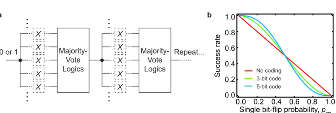
The errors in the classical computing can be represented by bit flips. A classical way to beat the errors is the repetition code (Figure 1.2a), where each bit is protected by a large number of its copies (0 → 000 . . . 0, 1 → 111 . . . 1), and error correction is performed repeatedly. By the end of each cycle, all copies are measured and a majority vote resets the bit with the most probable state. The success rate for preserving the original state in-creases as the number of copies grows, when the error probability per bit

perr <0.5 (Figure 1.2b). In the simplest case of three copies, 0 →000 and

1 → 111, the majority vote can protect the state when at most one copy has been corrupted in a cycle. The effectiveness of repetition code lies on the low probability for multiple errors to overturn the majority vote.

1.2 Quantum error and error correction 5 No coding 3-bit code 5-bit code Success rate 1.0 0.8 0.6 0.4 0.2 0.0 1.0 0.8 0.6 0.4 0.2 0.0

Single bit-flip probability, p_err X X X X X X X X X X Majority-Vote Logics Majority-Vote Logics Repeat... 0 or 1

a b

Figure 1.2: The classical repetition code. a, schematics of the classical repetition code. The dashed boxes indicate that bit-flip errors can happen on any copies with probabilityperr, during operations or idling.b, the success rate of the

major-ity vote as a function of the error probabilmajor-ity for each copy. The repetition code is useful whenperr <0.5, and a larger code can improve the performance.

accumulation of infinitesimal errors. A common error for a qubit isqubit

relaxation, as one state (|1i) is physically at higher energy and is subjected

to relaxation to the more stable one (|0i). An exclusively quantum error is

qubit dephasing, where a superposition state loses its ensemble coherence,

e.g., a state lying on the equator of the Bloch sphere turns into a mixture of states with different azimuthal angles. However, all errors can be posed into discrete errors with certain probabilities. Specifically, a decom-position can consist of only bit-flip errors,X, phase-flip errorsZ, and their combination Y = iXZ. In principle, we only have to fight against these two types of discrete errors.

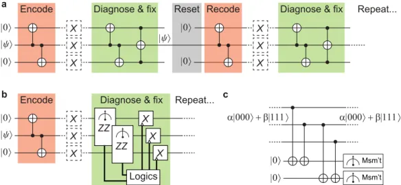
In the quantum repetition code, the quantum state is not copied but en-tangled with prepared ancillary qubits, bringing the redundancy required for error correction: the encoding process. The details of the encoding de-pend on which error one wants to protect from. For bit-flip errors, the state |ψi =α|0i+β|1i is mapped into a Greenberger-Horne-Zeilinger (GHZ)-type state α|000 . . . 0i+β|111 . . . 1i via CNOT gates. Note that quantum information is encoded in a 2-D subspace of a much larger Hilbert space. The majority vote is then implemented by a decoding step analogous to the encoding, followed by measurements of all ancillary qubits. The mea-surement outcomes diagnose whether a bit-flip has occurred on the orig-inal qubit or any of the ancillas, and apply the corresponding correction. A three-qubit version is shown in Figure 1.3a, where the majority vote can be achieved by a unitary gate: the controlled-controlled-NOT gate,

or Toffoli gate. Stemmed from the classical concept, the quantum

|〉 |0〉 |0〉 a _Repeat... |0〉 |0〉 |〉 Reset Diagnose & fix

X X X |〉 |0〉 |0〉

b _{Encode Repeat...}

X X X ZZ ZZ X X X Diagnose & fix

Logics

|0〉 |0〉

Msm’t

Msm’t

α|000〉 + β|111〉

c

Encode Diagnose & fix

X X X Recode

α|000〉 + β|111〉

Figure 1.3: Schematics of qubit repetition code for bit-flip errors. a, three-qubit bit-flip repetition code without measurements. The dashed boxes indicate the possible bit-flip errors. b, three-qubit bit-flip repetition code with stabiliser measurements and feedback corrections. The code repeats without decoding the logical state.c, implementation of theZZstabiliser measurements by entangling with ancillary qubits and measurements.

To protect against phase-flip errors, the protocol remains the same ex-cept for a basis transformation, as a phase-flip in z-basis is equivalent to a bit-flip in x-basis. This is realised by a Hadamard gates on each qubit; and the logical qubit is encoded inα|+ + +· · ·+i+β|− − − · · · −i, with |±i= (|0i ± |1i)/√2.

1.3 Physical implementations 7

three-qubit bit-flip repetition code, the codespaceα|010203i+β|111213iis

the common eigenstate of stabilisers Z1Z2 and Z2Z3 with eigenvalue +1

and+1, respectively. Note that they are just the parities of the excitations in the qubit pairs, with result even or odd. The corrupted codespaces by any bit-flip error, e.g., α|110203i+β|011213i, are still eigenstates of Z1Z2

and Z2Z3, with different eigenvalues (here, −1 and +1). For single

er-rors, the stabiliser measurements can correctly tell which corruption has occurred and correct it with feedback control∗ (Figure 1.3b). A stabiliser measurement can be implemented by entangling the qubit-pair with an-other ancillary qubit by CNOTs, and the measurement of this qubit reveals and stabilises the parity (Figure 1.3c).

This stabiliser-measurement-based bit-flip repetition code is the main focus of this thesis.

1.3

Physical implementations

A qubit can be realised in various physical systems. The required quantum two-level system can be polarisations or spatial modes of photon, spins of electrons or nuclei, specific atomic transitions, and specific levels of an ar-tificial atoms made of quantum electric circuits. While isolation of a qubit from its environment is essential to maintain coherence, interaction with the environment is necessary for manipulations, measurements and en-tanglement with other qubits. So what makes a qubit feasible for QIP? D. DiVincenzo answered this question with his famous criteria [15]: a scal-able system with well-defined qubits; the ability to initialise the qubits to a pure state; long relevant coherence times compared to the gate op-eration time; a universal set of gates; and qubit-specific measurements. Several physical platforms satisfy these criteria and have been amply de-veloped for QIP, such as nuclear magnetic resonance (NMR), linear optics, trapped ions and atoms, spin or charge quantum dots, nitrogen-vacancy (NV) centres in diamond, and superconducting quantum circuits. Al-though many of the records are set by the forerunners like trapped ions [16], solid-state architectures exhibit promising scalability and have ex-perienced a steady advancement [17–19]. Particularly, superconducting quantum circuits embrace the developed technologies in radio-frequency electronics and nanofabrication with semi- and superconducting materi-als. One of the most popular architectures of superconducting qubits is

circuit quantum electrodynamics (circuit QED). Inspired by the successful cavity QED in which natural atoms are controlled and monitored via pho-tons in a cavity or vice versa, circuit QED explores the coupling between qubits and microwave photons in resonators to protect, manipulate and measure the qubits, and to mediate interactions between qubits. Its flex-ibility in design allows to access the strong coupling regime of light and matter due to the small mode volume of light, and to even enter unprece-dented quantum regimes.

Despite the potentials, scaling up a quantum processor faces various challenges [20], including manipulation and readout of individual qubits while maintaining the coherences in all others, selective control of qubit-qubit interactions regardless of the coupling strengths and complexities, characterisation of a large-scale quantum process, closing the real-time feedback loop towards QEC, and many more. However, the universality of the circuit QED architecture and the increasing understanding of deco-herence resulting from noise or interactions, make the on-going progress optimistic.

In this thesis, we explore superconducting transmon qubits (section 2.1) in the circuit QED architecture.

1.4

Thesis objectives and overview

Although the concept of FTQC has been greatly explored, not even the simplest QEC protocol with fault-tolerant character has been experimen-tally realised. Previous demonstrations of QEC, using NMR [21], trapped ions [22, 23], linear optics [24], superconducting qubits [25], and NV cen-tres in diamond [26, 27] are inherently not fault-tolerant since the encoded information leaves the protected subspace between each decoding and re-coding step. Maintaining the encoded logical qubit in a protected sub-space is a prerequisite towards FTQC. A very first progress in this path would be the demonstration of QEC in the three-qubit repetition code using stabiliser measurements. The main difficulties lie in maintaining the multiple-qubit coherence during the protocol, and the single-shot fi-delity of the stabiliser measurements. With recent progress in the genera-tion of entanglement by parity measurement with superconducting qubits [28, 29], it is natural to extend the application of parity measurement as stabiliser measurement in a three-qubit space to demonstrate the simplest QEC protocol.

1.4 Thesis objectives and overview 9

QEC protocol, based on the initial tune-ups of the system by Dr. Olli-Pentti Saira, Dr. Visa Vesterinen, Dr. Stefano Poletto and Dr. ir. Diego Rist`e. We use a device with five transmon qubits at cryogenic temperature, three of which are the data qubits in which we encode a logical bit of information in the smallest QEC repetition code, and on which we perform double-parity measurement to detect bit-flip errors. The other two qubits serve as ancillas to implement parity measurements of the two pairs of data qubits. We achieve high single-shot readout fidelity for the projective measure-ments of ancilla qubits. Signalled by the ancilla results, the double-parity measurement projects the three-data-qubit state into subspaces stabilised by the measurement. We then show the generation of GHZ-type entan-gled state by this projection from a maximal superposition, and the gene-sis is witnessed to have genuine tripartite entanglement. We perform the stabiliser measurements on an encoded logical qubit corrupted by inten-tionally added bit-flip errors, showing their ability to discretise and detect the errors. In summary, we realize one round of the QEC repetition code, where we detect bit-flip errors, although we do not correct them.

Chapter

2

Circuit QED with superconducting

qubits

A basis element of superconducting quantum circuit is the LC circuit. It is a harmonic oscillator of the collective variables, charge and flux, and it can enter the quantum regime to give quantised excitations. But the transition energies are degenerate – isolated two-level systems are not ac-cessible. The necessity to realise a qubit is nonlinearity, here introduced by Josephson junctions. They serve as nonlinear inductances that are key to all designs of superconducting qubits. In this chapter, we introduce a specific type – the charge qubit, and its modern modification. We briefly formulate the interaction between qubit and cavity in the circuit QED ar-chitecture to illustrate the basic qubit gates.

2.1

The transmon qubit

2.1.1

From Cooper-pair box to transmon

Vg EJ,CJ

Cg CPB

Figure 2.1: Circuit representation of a Cooper pair box.A Josephson junction is represented by, with Josephson energyEJ and capacitanceCJ, the dashed box

indicates the CPB in which the Cooper pairs are isolated.

islands. The phenomenological Hamiltonian of the CPB is given by [30]

H_Q =4EC

∑

n−ng2|ni hn| −

EJ

2

∑

whereEC =e2/2CΣ (CΣ is the total capacitance, and here,CΣ =CJ +Cg),

ngmarks the charge offset set by the gate biasing, andEJ is the Josephson energy which is a measure of the coupling strength across the junction. The first term describes the Coulomb energy of the CPB and the second term describes the tunnelling of a Cooper pair through the junction.

The tunnelling energy closely resembles a tight-binding model in the band theory. We directly get a cosine-like dispersion−EJcosϕ, in the con-jugate coordinate by Fourier transform|ϕi =∑neiϕn|ni. From the Hamil-ton’s equation of motion

˙ˆ

ϕ=−∂H ¯

h∂nˆ = 4e2

¯

hCΣ n+ng

= 2e

¯

h V =Φ˙/Φ0, (2.2)

where ˆn = |ninhn|is the number operator andΦ0 the flux quantum, we

find ϕis directly related to the flux in the circuit, conventionally defined as Φ = Rt

−∞V(τ)dτ [30]. ϕ is shown to be the gauge invariant phase difference between the two islands of the junction.

The CPB Hamiltonian now has the celebrated form:

H_Q =4EC nˆ+ng2−EJcos ˆϕ. (2.3)

2.1 The transmon qubit 13

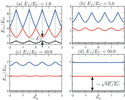
Figure 2.2: Gate-charge dispersion of the eigenenergies of charge qubits. Nu-merical calculations of the lowest three energy levels of a charge qubit are shown. In the transmon region (d), the energy dispersion with respect to the gate charge ngis exponentially decreased. Figure from [31].

hence low coherence time, which is the main obstacle for CPB. Although working at the chargesweet spotsof half-integerngeliminates linear noise sensitivity, stabilisation of the gate charge in a longer time scale required for robust measurements is still of great technical challenge.

The transmon (short forsuperconducting transmission line-shunted plasma

oscillation) qubit has been developed to resolve this problem by going to

the regime EJ EC, where the charge dispersion is exponentially sup-pressed, while the anharmonicityα≡ E01−E12(whereEmn ≡En−Em) is only reduced algebraically [31]. specifically, a first-order perturbation the-ory givesE01 =

p

8EJEC−ECandα = −EC. LargeEJ/ECcan be reached by shunting the junction with a large capacitor, increasingCΣ. Typically

it is achievable to have negligible charge dispersion while maintaining an anharmonicity that is large enough (∼300 MHz for qubit working at ∼6 GHz) for control pulses in nanosecond timescale.

2.1.2

Frequency tunability and flux biasing

qubit frequency.

In a general case where the two junctions are not identical, the Joseph-son Hamiltonian is given by

HJ =−EJ1cos ˆϕ1−EJ2cos ˆϕ2, (2.4)

where the phase differences across the two junctions ϕ1 and ϕ2 satisfy

ϕ1−ϕ2 = 2πn+2πΦ˜/Φ0 with integer n and magnetic flux ˜Φ through

the SQUID loop [32] (note that ˜Φis different from the flux variable of the circuit Φ). Defining ˆϕ = (ϕˆ1+ϕˆ2)/2 and the asymmetry d ≡ (EJ2−

EJ1)/(EJ1+EJ2), we have

HJ =− EJ1+EJ2cos

πΦ˜

Φ0

s

1+d2_tan2

πΦ˜

Φ0

cos(ϕˆ−ϕ0), (2.5)

where tanϕ0 = dtan(πΦ˜/Φ0) can be gauged out for constant magnetic

flux. The coefficient of the cosine term cos(ϕˆ−ϕ0) can be viewed as an

effectiveEJ for the double junction. It can be tuned fromEmax_J =EJ2+EJ1

to Emin_J = E_J2−E_J1

. Therefore the qubit frequency can be maximally

tuned for identical junctions. In general the asymmetryd is nonzero but small, and the minimal reachable frequency is low enough.

Experimentally the magnetic flux through the SQUID loop can be pro-vided by an external electromagnet or an on-chip constant current flow. The latter also allows fast changes in the flux and hence fast tuning of the qubit frequency.

Opening the tunability of frequency via magnetic flux also leaves the frequency susceptible to flux noise. Similarly, there exists flux sweet spots

where the linear dependence of the qubit dephasing time on the flux noise is eliminated [31].

2.2

Circuit quantum electrodynamics

2.2 Circuit quantum electrodynamics 15

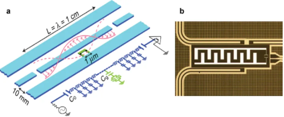
Figure 2.3: Schematic and example of circuit QED. a, basic structure of a double-junction CPB coupled to a transmission line resonator; the lumped circuit repre-sentation is also shown. Figure from [33].b, photograph of an example of current transmon qubits, coupling to three resonators. Note that a big shunting capaci-tor (white) helps to reduce EC and it capacitively couples to the antinode of the

resonator mode. Photograph courtesy: A. Bruno.

2.2.1

Cavity-qubit interaction

In circuit QED, a cavity is implemented either by a direct analogy of a 3-D microwave cavity, or by a 2-D coplanar waveguide (CPW) structure of a transmission line resonator.

We focus here on the transmission line resonator. It can be modelled as a series of an infinite number of LC circuits (Figure 2.3a) and essentially as an infinite number of coupled harmonic oscillators. The result is the har-monic eigenmodes with frequencies defined by the boundary condition. A standard quantisation gives the same Hamiltonian as a 1-D cavity [34]

Hr =¯h ∞

∑

k=0

ωk

a†_kak+1 2

, (2.6)

where a†_k and ak are the creation and annihilation operators of a cavity photon. In general, we are only interested in a specific mode, e.g., the fundamental modeωr =ω0and a=a0.

We consider now the interaction between a transmon and a cavity by capacitively coupling the two. The interaction energy arises from the charge potential across the junction induced by the electric field of the cavity mode. We have a Hamiltonian of the coupled system:

H =¯hωra†a+4EC nˆ −ng2−EJcos ˆϕ+βnˆ

a†+a, (2.7)

ge-ometry of the coupled system [31]. To simplify the physical picture, we in-troduce the transmon basis in which the transmon Hamiltonian is fully di-agonalisedH =_∑j¯hωj|ji hj|. With the coupling strength ¯hgij = βhi|nˆ|ji, the coupled Hamiltonian results in the form

H=h¯ωra†a+¯h

∑

j

ωj|ji hj|+¯h

∑

gij|ii hj|

a†+a. (2.8)

In the usual case whereωr ≈ωqandωr g, we can make the rotating

wave approximation (RWA) to ignore the terms that do not conserve en-ergy. Further in the qubit limit, considering only the lowest two transmon levels|↑i ≡ |0iand|↓i ≡ |1ias in a spin-1₂system, we redefine the energy offset and arrive at

H_JC =h¯ωr

a†a+1

2

+h¯ωq

2 σz+¯hg

a†σ−+aσ+

, (2.9)

where ωq = ω01 ≡ ω1−ω0, g = g01 = g10, σz is the Pauli operator, and σ± = (σx±iσy)/2 raises or lowers the spin. This is the Jaynes-Cummings

Hamiltonianwithout decay, which has been extensively used in cavity- and

circuit-QED. The swap-like coupling makes it diagonalisable, with ground state |↑, 0i and the dressed eigenstates |±,ni, where n denotes the total number of excitations. We obtain

|+,ni =cosθn|↓,n−1i+sinθn|↑,ni, (2.10) |−,ni =−sinθn|↓,n−1i+cosθn|↑,ni, (2.11)

wherenin the undressed states marks the photon number, and the dress-ing relies on the detundress-ing ∆q ≡ ωq−ωr: tan(2θn) = 2g

√

n/∆q. The

eigenenergies are

E↑,0 =−

¯

h∆q

2 , (2.12)

E±,n =n¯hωr±¯h

2

q

4g2_n+∆2

q. (2.13)

We will further discuss these in two distinctive regimes.

2.2.2

Qubit readout and number splitting

2.2 Circuit quantum electrodynamics 17

eigenstates |jiin a generalised Jaynes-Cummings Hamiltonian which re-sults from Eqn. 2.8 only taking RWA, we can apply a canonical transfor-mation ˜H = eSHe−S with S = _∑jλj|ji hj+1|a†−h.c., where the pertur-bative parameter λj = gj,j+1/(ωj,j+1−ωr). The result is a second-order

effective Hamiltonian [35]

˜

H=h¯ωra†a+h¯

∞

∑

j=0

ωj|ji hj|+χj,j+1|j+1i hj+1|

−

−ha¯ †a

"

χ01|0i h0| −

∞

∑

j=1

χj−1,j−χj,j+1

|ji hj|

#

, (2.14)

with the dispersive coupling χij = g2_ij/(ωij−ωr). Now taking the qubit

limit we obtain

H = ¯hω

0

q

2 σz+h¯ ω

0

r+χσza†a, (2.15) where the qubit frequency ωq0 = ωq+χ01 and the cavity frequencyω0r =

ωr−χ12/2 both experience the so-called Lamb shift, andχ=χ01−χ12/2.

It is clear from this expression that the cavity frequency depends on the qubit state. The photon frequencies corresponding to the two qubit states are separated by 2χ. The transmission or reflection signal of the cavity is therefore entangled with the qubit state, and a weak measurement of the cavity can determine the qubit state in a quantum non-demolition (QND) manner [33, 36].

In another perspective, the qubit frequency also depends on the photon number in the cavity. Grouping theσz terms we have

H=h¯ω_r0a†a+ ¯h 2

ω_q0 +2χa†a

σz. (2.16)

The qubit spectrum will split into separate peaks corresponding to differ-ent photon numbers in the cavity ifχ >γ, callednumber splitting[37, 38]. By driving at these number-selective transitions, we can entangle the qubit and a specific number state of the cavity. In other words, the qubit brings nonlinearity to the cavity, with which we can generate nonclassical pho-tonic states, such as Fock state with specific photon number, and macro-scopic quantum states – the Schr ¨odinger’s cat states – which are quantum superposition of coherent states [39, 40].

2.2.3

Qubit drive and single-qubit gates

the drive and the cavity can be modelled by capacitive coupling of two cavities as [34]

H_d =a+a† ξe−iωdt+ξ∗eiωdt

=aξ∗eiωdt+a†ξe−iωdt, (2.17)

where ξ defines the strength of the driving, ωd is the driving frequency,

and the second equality holds in RWA, which applies when the drive is not too strong.

The new full Hamiltonian becomes time-independent by moving into the rotating frame of the drive with an unitary transformation. Following Ref. [34], we have

H=h¯∆ra†a+h¯

∑

j

∆j|ji hj|+h¯

∑

gj,j+1

a†|ji hj+1|+h.c.+

+aξ(t)∗+a†ξ(t)

, (2.18)

where ∆r = ωr −ωd, ∆j = ωj−jωd, and ξ is now a slow function of time. Now the transmon states, the cavity and the drive are coupled in a complicated way. It is more informative to have an effective Hamiltonian with coupling directly between the qubit and the drive. This is done again by a canonical transformation with the Glauber displacement operator. We arrive at

H=h¯∆ra†a+h¯

∑

j

∆j|ji hj|+h¯

∑

gj,j+1

a†|ji hj+1|+h.c.+

+1

2

∑

∗₍

t)|ji hj+1|+Ω(t)|j+1i hj|

, (2.19)

whereΩ =2gα(t)(α(t) is introduced as the displacement in the Glauber operator that satisfies−iα˙(t) +δrα(t) +ξ(t) = 0). We note that Ω is the Rabi frequency of the swapping between |ji and |j+1i. Going into the dispersive regime discussed in the previous section, and considering the qubit limit, we have

H= ¯h∆

0

q

2 σz+h¯ ∆

0

r+χσz

a†a+ Ω∗(t)σ−+Ω(t)σ+

, (2.20)

where ∆_q0 = ω0_q−ωd and ∆0r = ω0r−ωd. The function of the drive is

2.2 Circuit quantum electrodynamics 19

of orthogonal quadratures, then we have Ω(t) = Ωx(t) +iΩy(t). The Hamiltonian becomes

H= h¯∆

0

q

2 σz+¯h ∆

0

r+χσz

a†a+ Ωx(t)σx+Ωy(t)σy

. (2.21)

Clearly, when the driving frequency is on resonance with the qubit fre-quency, i.e., ∆0_q = 0, we can have qubit rotation along any axis on the equator of the Bloch sphere by controlling Ωx and Ωy. Specifically, for a pulsed drive of duration τ, if Ωx = Ωπ and Ωy = 0 where Ωπ satisfies Rτ

0 Ωπ(t)dt = π, the pulse realises a π rotation along x-axis, or a bit-flip

gateX. We denote a rotation of angleθ along the axis on the equator with azimuthal angleϕasRθϕ.

As part of a universal set of gates for QIP, the Hadamard gate is of great interest, interchangingz-basis with x-basis. In principle, a real Hadamard can be realised by deliberately detuning the driving frequency, therefore introducing a σz term in the Hamiltonian (∆0q 6= 0) [33]. However, more

easily, it can be realised for specific input state by the qubit rotations ex-plained above. For instance, for the computational states inz-basis

H|0i= Rπ/2

Y |0i, H|1i=−R π/2 Y |1i,

where the minus sign in the second equation is irrelevant in the Bloch-sphere picture, but it reveals the inability to imitate a Hadamard with these rotations for a superposition state. Note for a sequence of Hadamard gates the replacing qubit rotations have to be carefully chosen. For example,

H·H|0i =Rπ/2

−Y ·R π/2

Y |0i, H·H|1i =R π/2

−Y ·R π/2 Y |1i.

2.2.4

Multiple-qubit gates

iSWAP gate

In the resonant regime of the Jaynes-Cummings interaction, ωq = ωr, the

dressed eigenstates are the maximal superposition of the undressed states with the same total excitation:

|±,ni = √1

2 |↓,n−1i ± |↑,ni

E±,n =nh¯ωr±hg¯

√

n. (2.22)

Rabi oscillation. In the generalised Jaynes-Cummings Hamiltonian where higher transmon states|ji are included, the Rabi oscillation occurs in any

m-excitation manifold, wherem =n+jwithnthe photon number. There-fore in the Hilbert space spanned by the states involved, the interaction gives a time evolution

U∝



  

1 0 0 0

0 cos(gt) isin(gt) 0 0 isin(gt) cos(gt) 0

0 0 0 1



  

, (2.23)

written in the basis {|j−1i |ni, |j−1i |n+1i, |ji |ni, |ji |n+1i}. For

t= π/2g, a so-called iSWAP gate is realised in them-excitation manifold:

iSWAP=    

1 0 0 0

0 0 i 0

0 i 0 0

0 0 0 1

   

, (2.24)

which fully swaps the excitation, while introducing a π/2 phase. This iSWAP between a qubit and a resonator is particularly important in this thesis (see section 3.3.2) and this resonator is called a bus. But in general, it is also interesting to have direct iSWAP between two qubits that are dispersively coupled to a common resonator, with an effective coupling strength

J = g1g2(∆q1+∆q2)

2∆q1∆q2 , (2.25)

with the subscripts 1, 2 denoting the two qubits. The iSWAP gate is of the same form withgreplaced withJ[35].

CPHASE gate

Mediated by a bus, the CPHASE gate between two qubits (1 and 2) can be realised by utilising the second excited state of the transmon [42]. We consider the case where both qubits are in|1i, therefore a CPHASE gate should introduce a π phase. Since the state of a qubit can be transferred back and forth into the lowest levels of a bus resonator using an iSWAP as explained above, the qubit excitation (e.g.,|12i of qubit 2) is temporarily

stored in|1Bi, where B denotes the bus. When we bring the 1-2 transition

of qubit 1 on resonance with the bus resonator,ω12 =ωr, coherent

oscilla-tion in the two-excitaoscilla-tion manifold between|1₁1Biand|210Biintroduces a

2.2 Circuit quantum electrodynamics 21

in the bus is transferred back to qubit 2, we have the CPHASE gate back in the two-qubit subspace:

CPHASE= 

  

1 0 0 0

0 1 0 0

0 0 1 0

0 0 0 −1



  

, (2.26)

up to some single-qubit phases result from the iSWAPs.

Chapter

3

Experimental Methods

3.1

Device and setup

3.1.1

The five-qubit processor

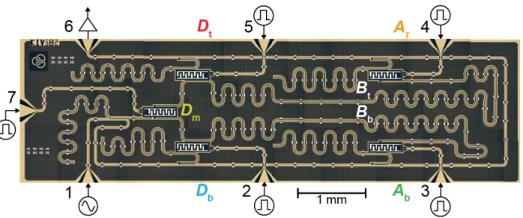
The five-qubit device is designed by Dr. O.-P. Saira and Dr. L. DiCarlo, and fabricated by Dr. A. Bruno. As depicted in Figure 3.1, the device consists of 12 quantum elements, including five transmon qubits (three data qubitsDt, Dm, Db and two ancilla qubits At, Ab), five quarter wave

CPW resonators dedicated to the readout of each qubit, and two half wave CPW resonators (indicated as Bt, Bb) serving as buses for the interaction

between qubits. Specifically, Bt couples the top qubits (Dt, Dm, At), and

Bb couples the bottom qubits (Db, Dm, Ab). A common feedline going

Figure 3.1: Photograph of the quantum processor. photograph courtesy: A. Bruno.

Table 3.1: Summary of the device parameters

Dt Dm Db At Ab Bt Bb

max f01(GHz) 5.755 6.181 6.788 6.002 6.452 4.80 5.52

operation point f01(GHz) 5.755 6.065 6.748 5.985 6.452 4.80 5.52

T1(µs) 7 13 6 9 10 7 6

T₂∗(µs) 3 2 4 3 0.7 13 11

T₂echo(µs) 7 13 5 4 3

g/2πtoBt(MHz) 78 48 – 51 –

g/2πtoBb(MHz) – 57 58 – 48

readout resonator fr(GHz) 7.599 7.787 7.998 7.095 7.086

χ/π(MHz) –0.6 –0.3 –1.0 –1.6 –2.0

κ/2π(MHz) 1.7 2.1 1.5 0.9 0.9

average assignment fidelity 89% 82% 95% 94% 95%

3.1.2

Electronics and cryogenics

A detailed diagram of setup connections is shown in Figure 3.2. The room temperature electronics involve a multi-channel current source, six mi-crowave sources and four arbitrary waveform generators (AWGs). All readout and qubit drive pulses are amplitude modulated sidebands of continuous wave (CW) carriers from microwave sources. The sideband modulation is done by a I-Q mixer with I and Q quadratures generated from two AWG channels. An AWG channel (sampling rate 1GS/s) covers sidebands at two qubit frequencies, therefore we use only 3 microwave sources to drive the five qubits, withDt and At,Dm and Ab sharing

3.1 Device and setup 25

Figure 3.2: Wiring diagram of the experimental setup.

ancilla qubits, with the same idea of sideband modulations. Split from the same sources, the same carriers are used as local oscillators to demodulate the output signal. A Delft-made current source maintains the flux-bias offset current defining the working frequency of each qubit, and on top of that, an AWG channel implements the fast control of qubit frequency. A dedicated microwave source provides the pump tone for the Josephson parametric amplifier (JPA) at low temperature [45].

the mixing chamber stage is achieved by low-pass filtering Eccosorb filters instead of dissipative attenuators, to avoid excessive heating in attenuat-ing direct current. The output of the feedline (port 6) is amplified by a JPA in a reflective mode while isolated from the pump tone and the amplified signal by a circulator and two extra isolators. Only the signals at the two ancilla-qubit frequencies are amplified by about 20 dB due to the limited bandwidth of the JPA. The output is further amplified by 40 dB by a com-mercial high-electron-mobility transistor (HEMT) amplifier at 3 K stage, and by 60 dB by two room-temperature amplifiers in series. The signal is split into multiple channels, two of which are demodulated by the two readout carriers respectively, and sent into the data acquisition card after a final amplification stage of 28 dB.

3.2

Characterisations of quantum elements

Parameters of the quantum elements in the five-qubit device are sum-marised in Table 3.1, including qubit frequencies, coherence times, and coupling strengths between elements. Spectroscopic measurements of all resonances in the system, from which coupling strengths and quality fac-tors are extracted, were performed by Dr. O.-P. Saira prior to this thesis. The methods are discussed extensively in previous theses (e.g., Ref. [47]), and will not be covered here.

3.2.1

Readout and initialisation

3.2 Characterisations of quantum elements 27

qubit in |0i. For the ancillas, however, the two dressed frequencies of the resonator are well resolved, therefore the measurement frequency lies in the middle of the the two (the bare resonator frequency), where the distin-guishability of the qubit states in the phase quadrature is maximised.

The ancilla readout signal is first amplified by a JPA at base tempera-ture, which is crucial to boosting single-shot readout fidelity for the sta-biliser measurements [49, 50]. A JPA can surpass the quantum noise limit, i.e., adding a noise less than half a quantum, by amplifying one phase quadrature of the signal while de-amplifying the other [51]. The JPA used in our experiment consists of a nonlinear media inside a superconducting CPW cavity [45]. The nonlinear media is realised by an array of SQUIDs and therefore its refractive index can be tuned by an external flux. The refractive index determines the frequency at which the signal will be am-plified. In the phase sensitive mode, an injected strong pump tone close to the signal frequency modulates the refractive index due to the non-linearity, therefore amplifies the signal which is in phase with the pump while deamplifying the signal that is out of phase. Tuning the phase of the pump tone can maximally discriminate the signals corresponding to the two states of the ancillas. We tune the JPA to have about 20 dB gain at the frequency 1 MHz detuned from the pump, close to the signal frequency of At. In addition, due to some hysteresis remained in the external

super-conducting magnet, a regular tuning of the amplified band of the JPA is necessary.

We actively initialise the quantum elements (five qubits and two buses) in their ground states before running a sequence. Four of the qubits (Dt,

Db,At,Ab) are initialised by measurement and post-selection on the ground

state result [50]. Dm, due to the lower readout fidelity, is initialised by

swapping its excitation with Bb prior to the initialisation of the buses,

based on that the original excitation inBb(∼1%) is almost negligible

com-pared to that of Dm (∼10%). The buses are then initialised by swapping

the photon populations with the initialised ancilla qubits, which are fur-ther measured and post-selected on their ground state to finally remove the excitations. Each quantum element has a residual excitation of 1∼2% after all initialisations.

3.2.2

Coherence times

The measurements of T1, T2∗ and T2echo of the qubits follow the normal

a

b

e

R_Xπ R_Xπ Msm’t

τ

R_Yπ/2 Msm’t

τ

R_Yπ/2

R_Yπ/2

c

R_Yπ Msm’t

τ/2

R_Yπ/2

R_Yπ/2 Rπ_Y Rπ/2_Y

τ/2

d

R_Xπ Rπ_X

τ

B_b

Msm’t

Rπ/2_Y R_Yπ/2

τ

Bb

Msm’t

R_Yπ/2 |0〉 |0〉 |0〉 |0〉 |0〉 |0〉 |0〉  Z 

Delay τ (ns)



Z



Delay τ (ns)

D_b D_b D_b  Z 

Delay τ (ns)

T2* = 3.6µs T1 = 7.9µs

T2echo = 4.9µs

A_b

A_b

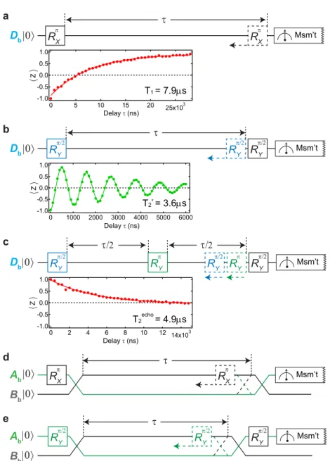
Figure 3.3: Measurements of the coherence times of qubits and buses. Dband Bbare taken as examples. a, sequence and typical data forT1 measurement of a

qubit. The dashed gate indicates the initial position in the scan of delay timeτ,

same in the following cases. b, sequence and typical data for T₂∗ measurement of a qubit. c, sequence and typical data forT₂echomeasurement of a qubit. Note that the refocusingπ pulse alongy-axis, instead of a conceptually-conventional

Rπ

X, brings the final state back to |0i. d, sequence forT1 measurement of a bus.

3.2 Characterisations of quantum elements 29

(Figure 3.3a). The average of measurement results reveals the excitation remained in the qubit. The qubit relaxation time T1 is obtained by a fit

with exponential decay.

The dephasing time T₂∗ characterises the coherence maintenance be-tween state |0i and |1i. Therefore, we prepare the qubit in the superpo-sition state (|0i+|1i)/√2 with a π/2 pulse, and a second π/2 pulse is applied after some delay time to ideally bring the qubit state to |1i to be measured, where the dephasing of the superposition state is reflected in the lost of population in |1i (Figure 3.3b). To avoid underestimating T₂∗

due to unavoidable, slight detuning of the drive, the qubit-drive frequency is intentionally detuned by a few MHz from the qubit frequency to see the Ramsey interference over delay time. An exponential fit to the decay of the oscillation amplitude givesT₂∗.

While T₂∗ shows dominantly the inhomogeneity in the qubit electro-magnetic environment, the intrinsic dephasing time, theoretically bounded byT2 6 2T1, is measured asT₂echousing Hahn echo technique. Aπ pulse is applied in the middle of the twoπ/2 pulses in the T₂∗ sequence (Figure 3.3c), and it will completely wash out the phase evolution due to the drive detuning or due to a static qubit environment. A simple exponential decay is measured in analogy to theT1measurement, but the decay ends up in a

50% mixture of the state|0iand|1i.

The coherence times of the buses can be measured in similar ways, making use of a qubit to prepare and measure the bus. For T1

measure-ment (Figure 3.3d), we prepare an ancilla qubit (At for Bt, Ab for Bb) in

state |1i, and with a iSWAP gate (explained later in section 3.3.2) the ex-citation is transferred into the bus (one photon). The residual exex-citation after a variable delay time is transferred back to the ancilla to be mea-sured. The residual excitation is limited by the fidelity of the iSWAP gates, but the decaying characteristic, hence theT1, is not affected. The bus T2∗is

measured similarly to that of a qubit, with the iSWAP gates transferring a superposition state (Figure 3.3e), and the bus T₂echocan be measured with an additional round-trip (by another two iSWAP gates) to the qubit state to be refocused by aπpulse in the middle of the sequence. We find theT₂∗ of a bus approaches the limit set by itsT1, therefore a T2echomeasurement

is not necessary and not shown.

a

b

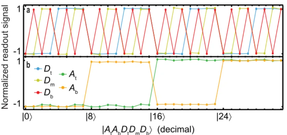
Normalized readout signal

1

-1 1

-1

D_{t A}

t

D_m

D_b Ab

|A_tA_bD_tD_mD_b〉 (decimal)

|0〉 |8〉 |16〉 |24〉

Figure 3.4: Low-crosstalk simultaneous qubit readouts. Averaged and nor-malised readouts of the data (a) and ancilla (b) qubits immediately after prepar-ing the five qubits in the 32 computational states.

any of the 0-1 or 1-2 transitions being too close to each other, and the de-grading of T₂∗ as the qubits are detuned from their sweet spots. Results of the overlapping transitions include cross-driving between qubits and readout cross-talk between qubits. We manually search for the optimal frequencies by fine-tuning the biasing DC in the flux lines, and the final working point of the qubits exhibits very low readout crosstalk (an assess-ment is shown in Figure 3.4), and reasonably good coherence times.

3.3

Gate tuning

3.3.1

Single-qubit rotation

The single-qubit rotation pulses (with rotation axis in x-y plane of the Bloch sphere, as shown in section 2.2.3) generally use the technique of Derivative Removal by Adiabatic Gate (DRAG) to minimise leakage into the second excited state|2i[52]. The DRAG pulse has a Gaussian envelop in one quadrature (I) and the derivative of this Gaussian in the other (Q). Therefore the tuning parameters include the frequency, the amplitude of the main Gaussian pulse, and the amplitude scale of the derivative with respect to that in the I quadrature (DRAG parameter).

Two of the qubits (Dt and Ab) also utilise the Wah-Wah (Weak

3.3 Gate tuning 31

0 5 10 15 20

1.0

0.5

0.0

-0.5

-1.0



Z



Number of π/2 pulses

|0〉 _{R RX}π/2 Msm’t

X π/2

R_Xπ/2 R_Xπ/2 R_Xπ/2 Rπ/2_X Rπ/2_X

3 pulses

5 pulses

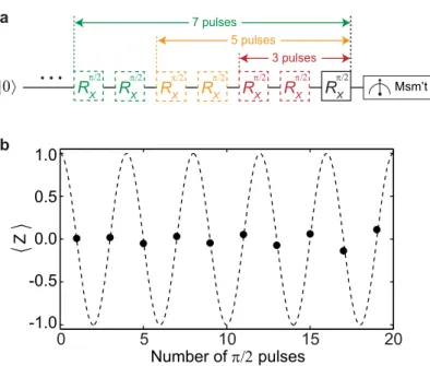
7 pulses a

b

Figure 3.5: Fine tuning of pulse amplitude. a, sequence for the fine tuning, where increasing odd number of π/2 pulses are applied. b, typical

measure-ments before pulse optimally tuned. Odd number of π/2 pulses always bring

the qubit onto the equator of the Bloch sphere, where the error in rotation angle is maximally revealed inhZimeasurement. The error accumulates over increasing number of pulses (measurements deviate from 0, black circle), and the period of a sinusoidal fit with amplitude bounded (dashed curve) infers the actual rotation angle of each pulse, therefore the correction.

to the 1-2 transition of Dm (Db), and aπ pulse of the former qubit causes

more than 10% population leakage into|2iof the latter when it is prepared in|1i. Wah-Wah pulses introduce two additional parameters, namely the amplitude and frequency of the modulation. When manually tuned up, Wah-Wah pulses reduce the leakage to less than 2%.

A preciser way to fine tune the pulse amplitude is applying an increas-ing number of consecutiveπ/2 pulses [56] (Figure 3.5). Even small ampli-tude imperfection will be revealed in the over-rotation after a large num-ber ofπ/2 pulses. The actual rotation angle of a single pulse can be deter-mined and therefore corrected much more precisely compared with using an AllXY sequence. In analogy, the DRAG parameter can also be tuned more accurately by a different combination of the consecutive pulses.

3.3.2

The iSWAP gate

The quantum buses play an important role in the processor, since there is no direct coupling between qubits and therefore any two-qubit gate is im-plemented between a qubit and a bus, which temporarily stores the quan-tum state of another qubit via an iSWAP gate [29, 57]. The fidelity of a two-qubit gate is partly limited by the loss of population and coherence in the two involved iSWAP gates.

As we have shown in section 2.2.4, when the qubit frequency is tuned in resonance with the bus mode, and if we limit ourselves in the one ex-citation manifold, the vacuum Rabi oscillation between|0Q1Biand|1Q0Bi

(where the subscripts denote qubit and bus) fully transfers the quantum state from the qubit to the bus or vice versa. An iSWAP gate is realised by turning on this interaction for half an oscillation.

The vacuum Rabi oscillation as a function of the detuning between the qubit frequency and the resonator mode is generally shown in a chevron

oscilla-3.3 Gate tuning 33

a

R_Xπ

R_Xπ

A_t

B_t D_m

Frequency

Length

Amplitude Msm’t

B

Msm’t R

π/2 R_Yπ/2

b

Q

|0〉

|0〉 |0〉

|0〉 |0〉

Figure 3.6: Tune-up of iSWAP gates. a, sequence for measuring the vacuum Rabi oscillations between a qubit and a bus, in either one- or two-excitation manifold. HereDmandBtare taken as examples. The black dashed line belowDmindicates

the 1-2 transition frequency ofDm; it is tuned downwards together with the qubit

frequency by the flux pulse. ForBtprepared in|0i, full vacuum Rabi oscillation

appears when the 0-1 transition ofDmis tuned on resonance withBt (transition

100-010 in Figure 3.7a). ForBt prepared in |1iby At, full Rabi oscillation in the

two-excitation manifold also appears when the 1-2 transition of Dm is on

reso-nance with Bt, with a smaller amplitude of the flux pulse (transition 110-200 in

Figure 3.7b). b, an assessment of the coherence preservation after two iSWAPs, angleϕis swept to reveal Ramsey oscillations.

tion is also most insensitive to the fluctuations in the pulse amplitude.

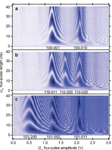
Figure 3.7: Vacuum Rabi oscillations betweenDmand the buses. Coherent

os-cillations betweenDm(prepared in|1i) and both buses, as a function of flux-pulse

amplitude (detuning of the qubit frequency) and duration (interaction time). The contrast in colour (white to dark blue) is the contrast in the measured qubit pop-ulation (|1ito|0i). The Buses are prepared in|BtBbi=|00i(a),|BtBbi=|10i(b),

and|B_tBbi=|01i(c). Transitions are labelled in the orderDmBtBb.

3.3.3

The CPHASE gate

The CPHASE gate is also implemented between a qubit and a bus. Fol-lowing section 2.2.4, we make use of the second excited state of the qubit (|2i). In the example shown in Figure 3.7a, Dm is prepared in state |1i

and Bt, Bb in |0i, and only the swaps with the empty buses are visible.

When Bt or Bb is prepared in |1i (by swapping one excitation from an

ancilla, see Figure 3.6a), additional Rabi oscillations in the two-excitation manifold appear as the 1-2 transitions ofDm cross the bus modes (Figure

3.3 Gate tuning 35

different coupling strength (hence a different oscillation frequency). A full oscillation between |1Q1Bi and |2Q0Bi (instead of a half oscillation in an

iSWAP) leaves the population in the qubit space but introduces aπphase, selective on the initial state |1_Q1Bi. A flux pulse on Dm turning on this

evolution implements the CPHASE gate.

Apart from the two-qubitπ phase we aim for, single-qubit phases are also present. During the flux pulse applied, Dm is detuned from the

ro-tating frame of its working frequency (driving frequency of the rotation pulses) and acquires a dynamical phase. A complete CPHASE gate be-tween two qubits comprises a CPHASE bebe-tween one qubit and a bus, sandwiched by two iSWAPs between the bus and the other qubit. Assum-ing ideal iSWAP gates, the experimental CPHASE gate in the two-qubit space is

CPHASE= 

  

1 0 0 0

0 eiϕ1 _{0 0}

0 0 eiϕ2 ₀

0 0 0 ei·(ϕ1+ϕ2+ϕ1,2) 

  

(3.1)

where the two-qubit phase ϕ1,2 is ideally π. The single-qubit phases ϕ1

and ϕ2 can be readily cancelled by a change of reference frame for each

qubit after the gate, through the calibration procedure shown in Figure 3.8.

Like an iSWAP, a resonant CPHASE as we described above requires a square flux pulse. This is important in the case of the CPHASE between

DmandBt, since the transition frequencies ofDmhas to cross theBb mode

to reach the Bt resonance. The sudden (non-adiabatic) tuning ideally

al-lows the crossing without leaving population in the Bb mode. In other

cases, “soft” flux pulses are used, which adiabatically detune the qubit frequency to acquire a two-qubitπphase in total [58]. The length of a res-onant CPHASE depends on the coupling strength (19 ns for the CPHASE betweenDmandBt), while the length of an adiabatic flux pulse is fixed to

40 ns in this experiment.

a

RX π

Bb D_m

Frequency

Db |0〉

|0〉

|0〉

RY π/2

R

π/2

Msm’t

1.0

0.5

0.0

-0.5

-1.0



Z



0 60 120 180 240 300 360

Angle  of Db (deg) b

0 1 |Dm〉

Figure 3.8: Tune-up of CPHASE gates. a, the sequence for tuning the CPHASE betweenDmandDbas an example, with an adiabatic flux pulse. Dmis prepared

in either |0i or |1i, indicated by the dashed gate. Angle ϕ is swept to get the

Ramsey oscillations in b, where the anti-correlation is obtained by tuning the flux-pulse amplitude. The dashed line indicates the angle at which a CNOT gate is realised withDmbeing the control qubit.

in superposition and the other in|0ior |1i. The Ramsey oscillation finds the point where the single-qubit phase is cancelled, and crucially, due to the CPHASE gate, the oscillation when the other qubit is in|0i, should be exactly out of phase with that when the other qubit is in|1i. The amplitude of the flux pulse is thus adjusted accordingly to have the exact opposite alignment.

In another perspective, this Ramsey-type experiment is better under-stood as tuning a CNOT gate, which is equivalent to a CPHASE gate sand-wiched by two Hadamard gates. As we have shown, two Hadamard gates are effectively replaced by an Rπ/2

Y followed by an R π/2

−Y. While the phase of the secondπ/2 pulse is swept, the two Hadamard gates are tuned when the qubit state is back to|0i, in case the other qubit (control-qubit) is pre-pared in|0i. A tuned CNOT gate will flip the state to|1iwhen the control-qubit is in|1i.

3.3.4

Phase errors induced by Stark effect

3.3 Gate tuning 37

0 45 90 135 180 −1

−0.5 0 0.5 1

0 45 90 135 180 −1

−0.5 0 0.5 1

0 45 90 135 180 −1

−0.5 0 0.5 1

0 45 90 135 180 −1

−0.5 0 0.5 1

0 45 90 135 180 −1

−0.5 0 0.5 1

0 45 90 135 180 −1

−0.5 0 0.5 1

0 45 90 135 180 −1

−0.5 0 0.5 1

0 45 90 135 180 −1

−0.5 0 0.5 1

0 45 90 135 180 −1

−0.5 0 0.5 1

0 45 90 135 180 −1

−0.5 0 0.5 1

0 45 90 135 180 −1

−0.5 0 0.5 1

0 45 90 135 180 −1

−0.5 0 0.5 1

0 45 90 135 180 −1

−0.5 0 0.5 1

0 45 90 135 180 −1

−0.5 0 0.5 1

0 45 90 135 180 −1

−0.5 0 0.5 1

0 45 90 135 180 −1

−0.5 0 0.5 1

0 45 90 135 180 −1

−0.5 0 0.5 1

0 45 90 135 180 −1

−0.5 0 0.5 1

0 45 90 135 180 −1

−0.5 0 0.5 1

0 45 90 135 180 −1

−0.5 0 0.5 1

0 45 90 135 180 −1

−0.5 0 0.5 1

0 45 90 135 180 −1

−0.5 0 0.5 1

0 45 90 135 180 −1

−0.5 0 0.5 1

0 45 90 135 180 −1

−0.5 0 0.5 1

0 45 90 135 180 −1 −0.5 0 0.5 1 Msm’t RY π/2

Target qubit |0〉 |0〉

Source qubit RX

θ

Source qubit

A_t A_b

D_t D_m D_b

Dt

Source qubit pulse angle θ (deg)

Target qubit  Z  At Dm Ab Db a b R π/2

Figure 3.9: Calibration of phase errors induced by Stark effect. a, the sequence to calibrate the phase error in atargetqubit, induced by driving asourcequbit. To determine the amplitude dependence, angle θ is fixed to0, π/4, π/2, 3π/4, or π, while angle ϕis swept to obtain Ramsey oscillations, whose phase shifts are

fitted to give the dependence. To obtain the assessment shown inb, the second

π/2 pulse on the targetqubit is fixed to Rπ_X/2, while the angleθ is swept from

0 toπ to linearly increase the pulse amplitude. The first Rπ_Y/2 leaves the target

qubit sensitive to dephasing, and the secondRπ/2

X reveals this phase error in the

which can result from any qubit-drive pulses and any excitations in the nearby quantum elements. As we have a single feedline, a qubit is in prin-ciple affected by the off-resonant driving pulses (for other qubits), during which the qubit frequency is shifted and a dynamical phase is acquired.

This phase error in each qubit can be accumulated and calibrated once for a whole sequence (a calibration sequence is explained in section 4.3.3). However, in a more dynamic sequence with varying number of pulses such as randomised benchmarking [59], this will be far from sufficient. A better solution is to correct the phase (or reference frame) of each pulse according the pulses applied before it. In other words, the reference frame of each qubit is updated after any pulse is applied. Since the Stark-shift-induced phased errors depend on the pulse intensity and detuning which is constant for a specific source, a calibration of the dependence of a qubit’s phase shift on the pulse amplitudes of other qubits is sufficient for generic phase-error cancellations. The phase errors on a targetqubit induced by pulses with different amplitudes (including Idling, π/4, π/2, 3π/4 and π) on a specific sourcequbit are measured as the phase shift of the Ram-sey oscillations of thetarget qubit with respect to the idling case (Figure 3.9a). The pulse-amplitude dependence of the phase error is obtained via a polynomial fit of the five data points.

Based on a previous model by Dr. V. Vesterinen, we implemented an automated scheme. After a sequence is designed, for a specific tar-getqubit, the time and the amplitude of all itssourcepulses are automati-cally recorded; and according to the calibrated dependences they are con-verted into phase errors of thetargetqubit, which are corrected by updat-ing the reference frame of the followupdat-ing drivupdat-ing pulses. A comparison of an assessment with and without this automated phase-error cancellation is shown in Figure 3.9b.

3.4

State tomography and entanglement witnesses

A direct way to characterise a quantum state would be analysing its den-sity matrix. In experiments, the measurables are the projections of single qubit states in certain measurement bases, and the correlations between the measurement results, such as the concurrence of the photon counts in certain polarisations in optics. We note that any density matrix can be de-composed into a linear combination of the Pauli operators, as in one-qubit space

ρ1Q =

1