Software developments in automated structure solution and crystallographic studies of the Sso10a2 and human C1 inhibitor protein

The handle

http://hdl.handle.net/1887/22715

holds various files of this Leiden University

dissertation.

Author: Waterreus, Willem-Jan

Title: Software developments in automated structure solution and crystallographic

studies of the Sso10a2 and human C1 inhibitor protein

in automated structure solution and

CRYSTALLOGRAPHIC STUDIES

of the Sso10a2 and human C1 inhibitor protein

Willem-Jan Waterreus

in automated structure solution and

CRYSTALLOGRAPHIC STUDIES

of the Sso10a2 and human C1 inhibitor protein

Proefschrift

ter verkrijging van

de graad van Doctor aan de Universiteit Leiden,

op gezag van Rector Magnificus prof. mr. C.J.J.M. Stolker, volgens besluit van het College van Promoties

te verdedigen op donderdag 5 december 2013

klokke 13:45 uur

door

Willem-Jan Waterreus

dr. Navraj Pannu (copromotor) prof. dr. Jaap Brouwer

dr. Remus Dame

prof. dr. Mathieu Noteborn

dr. Irakli Sikharulidze, Diamond Light Source, Oxford, UK prof. dr. Gerard Canters

Cover illustration reproduced with permission from:

Towards the Infinitesimal by Joan Modderkolk

Printed and bound by Wöhrmann Print Service, Zutphen, The Netherlands

The work reported in this thesis was performed at the Leiden Institute of Chemistry, Gorlaeus Laboratories, Einsteinweg 55, Leiden, The Netherlands. Funding was provided by the Netherlands Organization for Scientific Research (NWO), grant number 700.55.425 and Leiden University.

List of Figures vii

List of Tables viii

List of Abbreviations ix

1 Introduction 3

1.1 The importance of structural biology . . . 3

1.1.1 The molecular basis of life . . . 4

1.1.2 Protein structure and human disease . . . 5

1.2 An introduction to X-ray structure solution . . . 7

1.2.1 The basics of diffraction and the phase problem. . 8

1.2.2 Solving the phase problem. . . 12

Direct methods . . . 12

Molecular replacement . . . 13

Experimental phasing methods . . . 14

1.3 Automation in X-ray structure solution . . . 23

1.3.1 Substructure detection . . . 24

1.3.2 Substructure phasing . . . 26

1.3.3 Density modification . . . 27

1.3.4 Automated model building and refinement. . . 32

2 Recent advances in Crank 37 2.1 Introduction. . . 38

2.2 Recent developments in Crank . . . 40

2.2.1 Substructure determination . . . 40

2.2.2 Substructure phasing. . . 41

2.2.3 Density modification . . . 42

2.2.4 Automated model building and refinement. . . 42

2.4.1 Analysis of data sets that were not automatically

built . . . 47

2.5 Conclusions and future developments . . . 49

3 A new method for phase combination 51 3.1 Introduction. . . 52

3.2 Methods . . . 54

3.3 Results. . . 56

3.4 Discussion . . . 59

4 Structural analysis of DNA binding protein Sso10a2 63 4.1 Introduction. . . 64

4.2 Methods . . . 68

4.2.1 Cloning and overproduction . . . 68

4.2.2 Purification . . . 68

4.2.3 Crystallisation . . . 69

4.2.4 X-ray diffraction analysis . . . 70

4.2.5 Analysis of the crystal structure . . . 71

4.3 Results and Discussion . . . 71

4.3.1 Sequence analysis. . . 71

4.3.2 Structure solution . . . 74

4.3.3 Global structure . . . 77

4.3.4 Comparison of Sso10a and Sso10a2 . . . 77

4.3.5 Concluding remarks . . . 79

5 Crystallisation of human recombinant C1 inhibitor 83 5.1 Introduction. . . 84

5.2 Methods . . . 88

5.2.1 Protein expression and purification . . . 88

5.2.2 Crystallisation . . . 89

5.3 Results and discussion . . . 90

5.3.1 Crystallisation screening . . . 90

5.3.2 Diffraction targets . . . 91

5.3.3 Concluding remarks . . . 92

A Data sets used for testing 95

Bibliography 101

1.1 Bragg diffraction. . . 9

1.2 Diffraction image from the Sso10a2 selenomethionine data set 11 1.3 The Harker construction for a SIR experiment. . . 17

1.4 The Harker construction for a SAD experiment.. . . 19

1.5 Lack of closure in a SIR experiment. . . 21

1.6 The Harker construction for a MIR experiment.. . . 22

1.7 The Harker construction for a SIRAS experiment. . . 23

1.8 Typical steps in experimental phasing and model building.. . 25

1.9 Steps in traditional density modification. . . 28

1.10 Steps in statistical density modification. . . 31

2.1 Flow chart of the programsCrankinterfaces with.. . . 39

2.2 Screenshot of theCrank graphical user interface. . . 44

2.3 Fraction of the model built forCrank1.3 versus 1.4. . . 46

2.4 The Bijvoet ratios as a function of resolution for the peak and inflection wavelength data of the GerE data set. . . 48

3.1 Flow chart of the different steps in density modification. . . . 53

3.2 Map correlation forSAD-DM versus theσA. . . 57

3.3 Distribution of improvement in map correlation after density modification as a function of resolution and map correlation after experimental phasing for SAD-DM versusσA.. . . 58

3.4 Fraction of the model built correctly forSAD-DM versus σA. 60 4.1 Sequence alignment of archaeal Sso10a2 homologs. . . 73

4.2 Representative electron-density for each chain in asymmetric unit of the Sso10a2 crystal. . . 80

4.3 Superposition of the Sso10a and Sso10a2 structures. . . 81

3.1 Average fraction of the model correctly built forBuccaneer

and ARP/wARP. . . 59

4.1 Data collection statistics for Sso10a2. . . 74

4.2 Refinement statistics for Sso10a2. . . 76

A.1 The map correlation, fraction of the model built correctly and miscellaneous raw data comparing the performance of

Alba acetylation lowers binding affinity

ASU asymmetric unit

Bk2R bradykinin type 2 receptor

C1INH C1 inhibitor

DM density modification

EMSA electrophoretic mobility shift assay

ESRF European Synchrotron Radiation Facility

FOM figure of merit

fXIa activated factor XI

fXII factor XII

fXIIa activated factor XII

GAG glycosaminoglycan

GUI graphical user interface

HAE hereditary angioedema

HMWK high-molecular-weight kinogen

IPTG isopropylβ-D-1-thiogalactopyranoside

LMW1 low molecular weight rhC1INH species 1

LMW2 low molecular weight rhC1INH species 2

MLHL maximum likelihood Hendrickson-Lattman

MMT DL-malic acid, MES and Tris base

MR molecular replacement

NCS non-crystallographic symmetry

NMR nuclear magnetic resonance spectroscopy

PCB sodium propionate, sodium cacodylate and Bis-tris propane

PDB Protein Data Bank

PEG polyethylene glycol

PEG MME polyethylene glycol monomethyl ether

PNGase F peptide-N4- (N-acetyl-beta-glucosaminyl) asparagine amidase

RCL reactive center loop

rhC1INH recombinant human C1 inhibitor

RMSD root-mean-square deviation

SAD single-wavelength anomalous diffraction

serpin serine protease inhibitor

SIR single isomorphous replacement

SIRAS single isomorphous replacement with anoma-lous scattering

SPG succinic acid, sodium dihydrogen phosphate and glycine

TLS translation libration screw-motion

Introduction

1.1

The importance of structural biology

“It has not escaped our notice that the specific pairing we have pos-tulated immediately suggests a possible copying mechanism for the ge-netic material.” With this seemingly unassuming conclusion Watson and Crick (1953) have charmed many in the paper describing the double-helix structure of DNA. A model that elegantly explained X-ray diffrac-tion experiments on DNA fibres by Franklin and Gosling (1953). The discovery of the DNA double helix laid the foundation for a molecular understanding of heredity. While the relation between structure and function of a macromolecule may not always be so apparent, more often than not, a three dimensional atomic model gives valuable insight into the molecular basis for its biological activity. Only a few years after the discovery of the structure of DNA, Kendrew et al. (1958) published the first X-ray structure of a protein: myoglobin, an iron containing protein related to haemoglobin.

1.1.1 The molecular basis of life

Life is characterized by a number of innate unique qualities that set it apart from ordinary, lifeless matter. The self-organisation of well de-fined structural components into systems of enormous organisational complexity is the most ubiquitous property of life and required to per-form many of the functions that are also considered to be essential traits of living systems, such as the ability to interact with the environment, transform energy, metabolize matter, and reproduce (Palade 1964). At the heart of these processes are proteins whose function is determined by their molecular structure and composition.

The genes needed to produce all proteins are stored on either the strand of what is without question the best known structure of a bio-logical molecule: the DNA double helix. The amino acid sequence of a protein is encoded in a gene using a simple cypher consisting of a triplet of the bases adenine (A), thymine (T), cytosine (C), and guanine (G) (e.g. Lodish et al. 2000). The highly specific pairing of the A/T and G/C base-pairs, not only ensures that each strand can be reliably copied from the other, but also allows a gene to be converted into an RNA intermediate by a process called transcription. In the last stage of protein expression, each triplet in the RNA sequence is translated to the one of the twenty-one amino acids that can occur in a protein until a triplet signalling the end of the protein is encountered (e.g. Lodish et al.

2000).

introducing bends, or looping the DNA by intra-strand forming bridges (Luijsterburg et al.2008).

An important functional aspect of DNA packing is in the control of gene activity; usually local unpacking is associated with increased expression of the genes in that region and vice versa (Li et al. 2005; Luijsterburg et al.2008). In addition to the role in gene activity, chro-matin organisation has an important function in promoting the genomic stability, which is critical to survival and proliferation of an organism (Duboule et al. 2007; Oberdoerffer and Sinclair 2007). One example is the involvement of chromatin organisation and mobility in DNA damage repair. DNA lesions, caused by, for instance, UV- or ionizing radiation can have detrimental effects on the cell by blocking the transcription of the DNA into RNA, hindering DNA-replication or introducing muta-tions in the genetic code. While chromatin mobility was considered of little functional relevance, and chromatin packing often regarded as an obstacle to DNA repair, both are now recognized to have an active role in the repair of DNA lesions (Duboule et al. 2007; Groth et al. 2007; Misteli and Soutoglou2009; Soria et al.2012).

Homologous recombination, one of the processes involved in main-taining genomic integrity, sometimes inadvertently causes duplication of whole stretches of DNA. The genes duplicated through recombination or other mechanisms, can be passed on to an organism’s offspring and may diverge in function over time (Näsvall et al.2012; Ohno1970). In Chap-ter4the crystal structure of the Sso10a2 protein is presented, a member of three highly homologous DNA binding proteins that have co-evolved inSulfolobus solfataricus. Even though the structure of Sso10a2 is very similar to that of Sso10a, there are a number of striking differences. Chapter 4 speculates about the different functional role of Sso10a2 by comparing the structure with the homologous structure of Sso10a.

1.1.2 Protein structure and human disease

by molecular defects in proteins. Normal cellular activity is disrupted when a protein that performs an essential function is not active or not expressed, which in some cases can lead to serious disease.

The same processes that cause gene duplication can result in deletion of a gene and consequently reduce or completely abolish the expression of the encoded proteins. Various other types of mutation can affect protein activity either by disrupting the global fold, often the result of a frameshift or nonsense mutation, or by missense mutations that result in the substitution of a different amino acid. Especially when located in the hydrophobic core, an amino acid substitution can have a dramatic effect on the stability and global fold of a protein (Dill 1990; Eriksson et al.1992; Sharp1991), whereas localized changes in structure often have the greatest effect near the catalytic centre of an enzyme or in interaction sites (Schaefer and Rost 2012). Several diseases, such as familial Alzheimer’s and autosomal recessive Parkinson’s disease, are associated with mutations that decrease protein stability (Stefl et al.

2013; Wang and Moult 2001; Yue et al.2005).

While the substitution of an amino acid does not always lead to ap-preciable changes in the protein’s structure, the altered chemistry can have a marked influence on the activity of the protein. A well known example of such a mutation is the substitution of glutamic acid at posi-tion 6 by valine in haemoglobin that causes Sickle-cell disease in people homozygous for the mutation (Ingram1958; Neel1949). Under low oxy-gen conditions, a hydrophobic patch is exposed on the haemoglobin sur-face that binds the valine at position 6 resulting in the polymerization of haemoglobin into rod-like structures. The sickle shape and reduced flexibility of the red blood cells, induced by the fibrous haemoglobin pre-cipitates, causes blockage of capillaries. Consequently, the symptoms of sickle cell disease are mostly a direct result of restriction of blood flow to organs and tissues.

the biological function of an inactive protein can sometimes be accom-plished by simply substituting it with an active equivalent. For instance, hereditary angioedema (HAE), a condition which is accompanied by life-threatening swelling in the upper airways, may be treated by substi-tuting endogenous inactive or absent C1 inhibitor (C1INH) though in-travenous injection of Ruconest®, a recombinant C1INH (Plosker2012; Varga and Farkas2011; Zuraw et al.2010). Chapter5 reports the out-come of a high-throughput crystallization screen of three forms of recom-binant human C1 inhibitor (rhC1INH) in over one thousand different conditions. Several high quality crystals were obtained and preliminary evidence suggests that these crystals may contain rhC1INH in a confor-mation that is currently unknown. Knowledge of both active and latent (Beinrohr et al.2007) forms of C1INH will give insight into the molecular mechanisms underpinning C1INH’s activity, and could provide a molec-ular explanation for HAE and other diseases associated with molecmolec-ular defects in C1INH.

1.2

An introduction to X-ray structure

solution

struc-ture solution strategies and obtain a three dimensional model from even the most challenging diffraction data.

1.2.1 The basics of diffraction and the phase problem

The behaviour of X-ray photons can be understood in terms of properties associated with waves, as well as particle-like properties. When an X-ray photon interacts with an electron bound to an atomic nucleus it can scatter elastically. This means the energy of the photon, and thus its wavelength, is conserved and only the direction of the photon is changed. Alternatively, X-ray scattering can be thought of as the interaction of electromagnetic waves with the electrons in a solid material. Irradiation of the solid with an X-ray beam causes the electrons to oscillate with the same period as the incoming beam. The accelerated electrons emit their own electromagnetic field with the same phase and wavelength as the incident X-rays that propagates radially outward from every scatterer. The resultant field composed of contributions of individual scatterers is called the scattered wave.

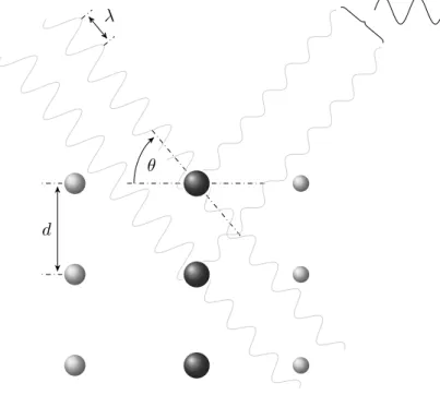
Due to the periodic structure of a crystalline solid, diffraction of X-rays by a crystal can be described as scattering of electromagnetic waves by a series of equidistant planes, denoted by three integers h, k and `, known as Miller indices (Miller 1839). As illustrated in Section1.2.1the incident X-ray beam hitting the surface of an (hk`) plane at angleθ is partially scattered at the same angle θaway from the plane. The non-scattered radiation is transmitted deeper into the solid until it interacts with the electrons in the second plane, where the process repeats. The X-rays reflected off a given (hk`) plane will travel different path lengths through the solid. Constructive interference of the scattered waves only occurs at certain angles θ for which the path lengths are equal to an integer number n times the wavelength λ. This relationship, shown in Equation 1.1 was derived by William Lawrence Bragg and is known as Bragg’s law (Bragg 1913).

θ

d

λ

Figure 1.1: Bragg diffraction. At the given angle of incidenceθ _the

X-rays scattered off the parallel (hkℓ_{) planes separated by a distance}d_are

shifted in phase such that they interfere constructively and give rise to a detectable reflection. For most other values of θ _{the reflected waves}

The distance between successive identical planes in the crystal is denoted by d. It is immediately apparent from the reformulation of Bragg’s law shown in Equation 1.2 that the maximum resolution at which a crystal can be sampled, that is the minimum distance dmin be-tween (hk`) planes, is determined byθmax, the maximum angle to which the crystal still diffracts. Theoretically the maximum resolution would be obtained when θmax = 1₂π, but due to decreasing atomic scattering factors at increasing Bragg angles the maximum scattering angle is lower (θmax 1₂π).

dmin = 1₂ nλ

sin(θmax) (1.2)

In a diffraction experiment the angle of the primary X-ray beam with respect to the crystal planes is changed by rotating the crystal. Whilst rotating, the position and intensity of the diffracted waves are recorded on an X-ray detector. The result is a regular arrangement of spots of varying intensity, known asreflections (see Section1.2.1). Each reflection can be assigned a set of indices (hk`) associated with the direction of the set of reflecting parallel planes in the crystal. The type and number of scattering atoms in the (hk`) planes, or more precisely the associated electrons, determine the magnitude of the corresponding (hk`) reflection. The squaredstructure factor amplitude is proportional to the intensity value of a reflection |Fhk`|2 ∝Ihk`.

Fhk` =|Fhk`|eiαhk` = N

X

j=1

fje2πi(hxj+kyj+`zj) (1.3)

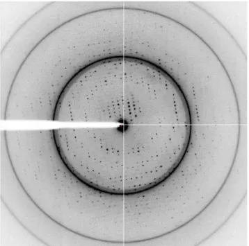
Figure 1.2: Diffraction image from the data set used to solve the Sso10a2 structure presented in Chapter4. Each dot represents a reflection that is assigned an (hk`) index. The structure factor amplitude |Fhk`| is calculated from the intensity valueIhk` of each reflection. Most X-rays pass through the crystal without being scattered, which shows up as a large high intensity circle in the centre of the image. The further away from the centre the reflections are, the higher the resolution of the data set. Some of the reflections are obscured by the large ring around 2.2 Å, a problem that results from scattering by the ice that can accumulate on the crystal.

that the structure factors are areciprocal spacequantity as the Miller in-dices are actually derived from the fractional numbers 1/h,1/k and 1/` denoting the intersections of the associated lattice planes with the unit cell axes. By applying a Fourier transform to Equation 1.3 the recip-rocal space may be transformed to real space leading to the following relationship.

ρ(xyz) = 1 V

X

hk`

As mentioned earlier the structure factor amplitudes are propor-tional to the square root of the intensity |Fhk`|2 ∝ Ihk`. However, the phase αhk` in Equation1.4cannot be measured experimentally and methods are needed to estimate the phase. This is known as the phase problem in crystallography.

1.2.2 Solving the phase problem

Below, three methods to solve the phase problem in X-ray crystallogra-phy are discussed: Direct methods refer to mathematical methods that try to estimate the phases of the Fourier transform of the scattering den-sity from the corresponding structure factor amplitudes alone. Another increasingly popular method in macromolecular X-ray crystallography is molecular replacement, which makes use of a similar structure to the structure one is trying to solve to obtain the initial phase estimates. The third family of methods exploit the scattering by one or more heavy atoms in the crystal to obtain the phases. These effects consider ad-ditional information from crystals containing a heavy atom that can be measured experimentally and are hence referred to as experimental phasing methods.

Direct methods

lead to a solution unless at least half of the theoretically measurable reflections in a 1.1 to 1.2 Å range are observed. This empirical rule, which has come to be known as “Sheldrick’s rule”, was given a struc-tural basis for proteins by Morris and Bricogne (2003) who argue that the rule has its origin in bonding distances typical of such molecules and the occurrence of families of inter-atomic distances that differ by 1.1 to 1.2 Å. Resolutions above 1.2 Å however are seldom attained in macro-molecular X-ray crystallography. Moreover, the application of classical direct methods is limited to structures of several hundred non-hydrogen atoms. The advent of dual space iteration methods as implemented inSnB(Rappleye et al.2002) andSHELXD(Schneider and Sheldrick

2002) allows larger structures up to a few thousand non-hydrogen atoms to be solved (Usón and Sheldrick1999) and is enhanced by the presence of intrinsic metal ions or other heavy atoms (Weeks and Miller1999). Nonetheless direct methods are of limited practical use in protein crys-tallography, with the exception of the determination of the heavy-atom substructure in experimental phasing methods, discussed in more de-tail in Section 1.3.1. Perhaps the combination of direct methods with other phase improvement procedures may relax the resolution restraints somewhat and allow larger structures to be phased in the future.

Molecular replacement

Molecular replacement (MR) leverages the abundance of structural in-formation present in the PDB to solve a new structure. An initial elec-tron density map is obtained by combination of the structure factor amplitudes of the unknown structure with the phase information of one or more known structures that are believed to have a similar fold. As a rule of thumb MR has a good chance of being successful if the unknown structure has more than 25 % sequence identity with the MR search model and their Cα _{atoms have a root-mean-square deviation smaller} than 2.0 Å (Giorgetti et al.2005; Taylor 2010).

new structure. Instead of exploring six-dimensional space for the cor-rect solution, many programs split this problem into finding the right rotation and translation separately. Classically, these search methods employ the Patterson function shown in Equation 1.5.

P(uvw) = 1 V

X

hk`

|Fhk`|2cos(2π(hu+kv+`w)) (1.5)

Generating a Patterson map does not require knowledge of the phases and can simply be calculated from the squared structure fac-tor amplitudes, which are proportional to the intensities. The peaks in a Patterson map correspond to interatomic vectors, that is for a crystal with N atoms in the unit cell the map has N(N −1) maxima. This

high-density of peaks and the partial overlap due to thermal vibration of the atoms makes it impossible to generate distance restraints for all atoms in case of larger structures like proteins. However the correla-tion of a Patterson map of the experimental data with Patterson maps of a MR search model in different orientations can be used to find the correct rotation (Crowther 1972; Rossmann1990). Similarly, Patterson-based methods can be used to find the appropriate translation of the origin and using the self-rotation function non-crystallographic symme-try (NCS) can be identified. The phases calculated from the correctly oriented MR search model are used to generate an initial electron density map for the new structure. These phases can be subsequently improved by model building iterated with refinement.

The MR approach is so powerful that to date nearly two-thirds of the structures deposited in the PDB have been solved1 _{by MR. As the} size of the PDB continues to grow so will the probability that a given new structure can be solved by MR.

Experimental phasing methods

The use of heavy-atom derivatives was amongst the first methods em-ployed to solve the phase problem in protein crystallography (Kendrew

1

et al. 1958; Perutz 1956). The method relies on the intensity differ-ences between the native protein crystal and an isomorphous heavy-atom derivative to obtain the correct phase of the native protein structure.

Heavy atoms, such as lanthanides, (transition) metals, can be in-troduced into a protein crystal by soaking it in a solution containing a heavy atom salt. Frequently these heavy-atoms bind on well defined places in the protein. For instance Hg2+ _{ions bind the cysteine thiol}

groups and uranyl salts like UO₂NO₃ preferentially bind between the carboxyl groups of glutamic acid and aspartate. Other examples in-clude Pb and PtCl2–

4 -ions that bind cysteine and histidine, respectively

(e.g. Rould1997).

The use of heavy atom solutions, however, carries one major practical downside. Many of substances containing heavy atoms are highly toxic, which in combination with the tendency of many of these compounds to accumulate in the human body, poses a health risk to exposed workers. Noble gases, such as Xe, are non-hazardous heavy atoms that can be introduced into the crystal in a high-pressure environment. Note, that there is no guarantee that an heavy atom can even be introduced in the crystal. In fact often crystals are seen to disintegrate in the heavy atom soaking solution. When the effect on the crystal packing is more subtle, poor diffraction compared to the native crystal can be the result.

The intensity differences arising from incorporation of a heavy atom are relatively easy to determine, considering a single Hg atom in a 1000 atom protein can give a fractional change in intensity of as much as 25 % (Crick and Magdoff1956; Taylor2010).

Defining the structure factor obtained from both heavy atoms and protein as the derivative structure factorFP H and assuming it is a vec-tor sum of the nativeFP and the heavy atom FH structure factor, an initial estimate of the heavy atom structure factor amplitude may be obtained with the following approximation: |FH| ' |FP H| − |FP|. Using

of the heavy atoms in the unit cell may be obtained by direct methods (see Section 1.3.1). Once the heavy atom substructure is known the heavy atom coordinates and other parameters such as thermal B-factors and occupancy can be refined to give a more accurate estimate of the heavy atom structure factor FH and consequently the phase ofFP.

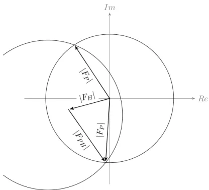
In an error-free, idealized experiment, obtaining the native protein phase is a simple geometric problem that is solved by applying the cosine rule shown in Equation1.6, which leads to two possible solutions forαP that are distributed symmetrically about the heavy atom phase as is illustrated by the Harker construction shown in Figure 1.3.

αP =αH±arccos

F_{P H}2 −F_P2 −F_H2

2FPFH (1.6)

Isomorphism of the heavy atom derivative is a critical condition to the success of phase determination by isomorphous replacement that may not be met. A seemingly small change in unit cell dimensions, ori-entation of the protein in the unit cell, or other form of non-isomorphism result in intensity differences that interfere or completely mask the signal from the heavy atom(s) alone (Crick and Magdoff 1956). Non-isomorphism can be caused by the soaking process itself, that, in many cases causes shrinkage of the crystal by dehydration due to the difference in osmotic concentration between the mother liquor and the heavy atom solution. Furthermore. soaking can induce reorientation and changes in conformation of the protein, as well as exchange of salt-ions other than the heavy atoms.

scat-Re Im

|FH|

|_F

P_|

|

FP

|

|_F

P H_|

Figure 1.3: The Harker construction for a single isomorphous replace-ment (SIR) experireplace-ment. The circles indicate possible values for the phase. In the idealized case there are two possible choices for the phase, found where the circles intersect. However, in reality one needs to ac-count for errors in the measurements and in the atomic parameters and the possible phase is smeared out.

tered normally when interacting with the electron cloud surrounding the atomic nucleus it may also be absorbed and promote an electron from an inner shell. The absorbed photon can be re-emitted at a lower energy, known as fluorescence; immediately re-emitted at the same energy; or retarded compared to the normally scattered photon. The latter can be modelled by the addition of an imaginary component to the photon’s phase represented by theif” term in Equation1.7.

The scattering behaviour of individual atoms is given by the atomic scattering factor f shown in Equation1.7. In the simplified description the wavelength dependent contributions f0 and f00 can be ignored and the scattering factor only depends on the Bragg angle θ and Friedel’s law holds.

Re Im

|_F

H| f

00 f 00

|FP H(−)|

|_F

P H

(−

)|

|_F

P H₍₊₎

| |FP H(+)|

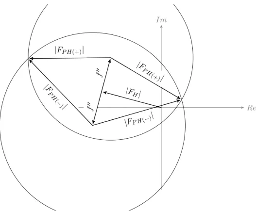
Figure 1.4: The Harker construction single-wavelength anomalous diffraction (SAD) experiment. In the presence of an anomalous scat-terer Friedel’s law breaks down. Thef00 term is advanced 90° in phase, which gives rise to the Bijvoet difference ∆F± =|FP H(+)| − |FP H(−₎|. If the measurement errors are ignored, the phase choices are given by the intersections of the phase circles.

Nowadays high-efficiency selenomethionine labelling protocols are available for bacterial, yeast, insect and mammalian cell expression sys-tems (Barton et al.2006). The major advantage of selenium over sulphur in SAD and multiple-wavelength anomalous diffraction (MAD) phasing is that the selenium absorption edge (0.9795 Å) is within 1.5 to 2.5 Å the typical range at a tunable macromolecular beamline (Doutch et al.

An idealized error-free SIR or SAD experiment would both result in two possible choices for the phase, only one of which is correct. This phase ambiguity cannot be resolved without introducing additional in-formation. An earlier procedure to address the phase ambiguity is the re-solved anomalous phasing approach, as used by Hendrickson and Teeter (1981) to solve the crambin structure, which uses the combined probabil-ity resulting from the partial structure and from anomalous scattering, unless the latter gives rise to a strong unimodal phase probability dis-tribution. An alternative approach to choose the right set of phases is based on direct methods and employs the relations between large nor-malized structure factors to refine the initial phase estimates (Fan et al.

1990; Hauptmann 1982, 1996). Finally, the iterative single-wavelength anomalous scattering method introduced by Wang (1985) starts from the average phase and enhances meaningful features in the macromolecular crystal through iterative real-space smoothing of the electron density in the solvent region, much like ordinary solvent flattening in density modification (DM).

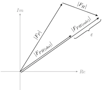
Another difficulty associated with phase determination by the SIR or SAD is that the initial phase estimates are often simply too inaccu-rate to geneinaccu-rate an electron density map with interpretable features, or even one that could be improved by density modification. This inac-curacy has its origin in the experimental errors in the measurement of the structure factor amplitudes, errors due to scaling, non-isomorphism, errors in heavy atom parameters or even that the isomorphous and/or anomalous signal is not strong enough.

Re Im

|FPH( obs)

|

|FPH( calc)

| |F_H|

|FP |

ε

Figure 1.5: The lack of closureεbetween the calculated derivative struc-ture factor amplitudeFP H(calc)and the observedFP H(obs)illustrated for a SIR experiment.

ε=|FP H(obs)| − |FP H(calc)|=|FP H(obs)| − ||FP|eiαP +|FH|eiαH|| (1.8) In the case of a SIR experiment the phase probability distribution is obtained as shown in Equation1.9. This assumes the measurement er-rors are contained in the derivative structure factor amplitudeFP H(calc) and follow a Gaussian distribution (Blow and Crick1959). The lack of closure varianceE2 is given by Equation 1.10.

P(αP)∝e−ε 2_/2E2

(1.9)

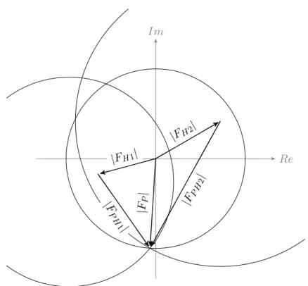
E2 =h(FP H(obs)−FP H(calc))2i (1.10) Collecting additional data, in the form of MAD data or several heavy-atom data set, is often worthwhile. As illustrated in Figure 1.6

sharp-Re Im

|FH1|

|FH2

|

|

FP

|

|_F

P H

1|

|FP

H2

|

Figure 1.6: The Harker construction for a multiple isomorphous replace-ment (MIR) experireplace-ment. The additional heavy atom derivative restricts the phase from two in the case of SIR to a single choice.

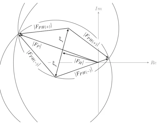
Re Im

|F_H| f

00 f 00

|F_P|

|FP H(−)

| |_F

P H

(−

)|

|_F

P_H

(+)_|

|FP H(+)|

Figure 1.7: The Harker construction for a SIRAS experiment. The phase choices are restricted from two options for SAD to one choice by the combination isomorphous replacement and anomalous data.

the phase circles in a MAD Harker diagram have only one intersection. The added benefit of MAD is that the data can be collected on a single crystal.

1.3

Automation in X-ray structure solution

orPhenix (Adams et al.2010), that use sensible default settings and a high degree of automation allow non-crystallographers to solve a crys-tal structure. Secondly, X-ray cryscrys-tallography technology has matured to a stage where it is being deployed in structural genomics consortia across the world for high-throughput structure determination. The large number of diffraction experiments performed by such consortia call for automation of data processing to enable efficient evaluation of candidate data sets for structure solution.

Many research groups involved in development of software for macro-molecular crystallography are attempting to provide fully automated programs for structure solutions by integrating MR strategies, pipelines for structure solution from experimentally obtained phase estimates, and increasingly combinations of both. Structure solution from phase estimates obtained from an anomalous scattering or isomorphous re-placement experiment always follows the same basic separation of steps shown in Figure 1.8even though the programs used may differ.

1.3.1 Substructure detection

Solving a structure by experimental phasing rests on the ability to suc-cessfully detect the anomalous substructure. Without it, calculation of substructure phases is impossible. Even if the phases recovered from the substructure cannot be extended to the full model automatically, it is clear that if substructure detection is successful there is some anomalous signal that may be exploited to provide better phase estimates, by for instance combination with phase information from MR or DM.

Substructure factor amplitude estimation

Substructure detection

Phasing

Density modification

Model building & refinement

Figure 1.8: Typical steps in the (automated) solution of a macromolec-ular crystal structure by experimental phase determination. In contrast to phasing by molecular replacement the initial phase estimates are re-covered from the anomalous scattering component, or the isomorphous difference between a native- and heavy atom derivative data set.

for determining the substructure for MAD and MIR.

the tangent formula (Karle and Hauptmann 1956). The map obtained by combination of the improved phases with the normalized structure factors is searched for the highest peaks that could be possible atoms. Several different approaches exist for the real space, or ‘baking’ part of the ‘Shake-and-Bake’ routine (Usón and Sheldrick 1999). The pro-gram SnB implements the dual-space iteration algorithm in its purest form, though most substructure detection programs, such asSHELXD, HySS (Grosse-Kunstleve and Adams 2003) and SIR2011(Burla et al.

2012) employ a hybrid approach combining ‘Shake-and-Bake’ type pro-cedures, other direct methods inspired approaches, as well as Patterson based procedures. A noteworthy exception is the program Crunch2 (de Graaff et al. 2001), which takes a different approach to ‘Shake-and-Bake’ that is based on Karle–Hauptman determinants (van der Plas et al. 1998).

1.3.2 Substructure phasing

Obtaining accurate initial experimental phases estimates is an important aspect of automated structure solution pipeline. Advanced maximum-likelihood methods offer substantially better models of an anomalous scattering or isomorphous replacement experiment and associated errors. The univariate Gaussian phase probability defined by Blow and Crick (1959) was an important conceptual advance in thinking about phase estimation and modelling errors. Many researchers expanded on the lack of closure work using more advanced probabilistic models based on the maximum-likelihood formalism. The first step in this direction was taken by Otwinowski et al. (1991) who, inMlphare(Collaborative Computational Project Number 41994; Otwinowski et al.1991), applied the phase probability as a weight in heavy-atom refinement as well as during the structure factor calculation. In contrast to many others at that time who used only one phase for each reflection to estimate the heavy-atom parameters.

phases and the “true” structure factor amplitude which, for example, is not measured in a SAD or MAD experiment. While the program refines errors, scale and atomic parameters simultaneously with a Gaus-sian error in the isomorphic and anomalous terms, it does not consider correlations between data sets and errors. In contrast, the programBp3 (Pannu and Read2004) directly considers the correlations between data sets and correlated errors for a SAD experiment, which has shown to be better over other approaches.

1.3.3 Density modification

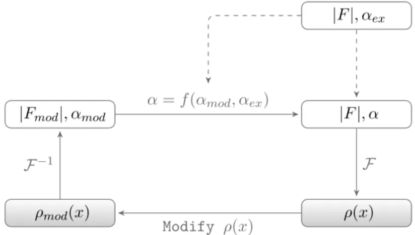
The experimentally phased electron density map may initially be of insufficient quality to allow automatic tracing of a three dimensional atomic model. DM aims to improve phase estimates with an itera-tive procedure that cycles between real space incorporation of chemical knowledge and combination of the real space modified phases or phase distributions with the experimentally obtained phase probabilities in reciprocal space.

Figure1.9 illustrates DM in its most traditional form, starting with the generation of the electron density map by Fourier summation of the structure factors calculated with the centroid phases from the experi-mentally obtained phase probabilities (see Equation1.4). Three proce-dures frequently used to modify the resulting electron density map are solvent flattening (Leslie 1987; Wang 1985), NCS averaging (Muirhead et al.1967) and histogram matching (Zhang et al. 1997).

|F|, αex

|F|, α

ρ(x) ρmod(x)

|Fmod|, αmod

F

Modify ρ(x)

F−1

α=f(αmod, αex)

Figure 1.9: Steps in traditional density modification. Structure fac-tor amplitudes, phases and electron density are indicated with |F|, α and ρ(x), respectively. The updated phase probabilities are obtained by multiplication of the original phase probabilities with the modified phases weighted according to the agreement between original and mod-ified structure factor magnitudes.

the electron density to distinguish solvent and protein, the solvent mask may be defined by looking at local variance throughout the unit cell. Indeed, the featureless solvent region will have a low variance compared to the regions with protein. In the flattening stage, the electron den-sity in the solvent region is set to the average solvent denden-sity, effectively removing the noise not associated with any structural information.

of the electron density the histogram is made to look more like that of a well phased map. This suppresses negative electron density and tends to sharpen electron density peaks (Cowtan2010).

Note that the application of scaling and masking functions in real space is equivalent to combining, in reciprocal space, many structure factors through a convolution. This is an intrinsic property of the re-lation between reciprocal and direct space by Fourier transformation. Consequently, the random error component of the structure factors will average out, whereas the true values of the structure factors will add up systematically.

After modification of the electron density map the modified struc-ture factors, obtained by inverse Fourier transform, need to be com-bined with the experimental phase probabilities. Because there is no explicit modified phase probability distribution, one is generated by es-timating the errors in the density-modified phases from the agreement from the between the observed and modified structure factor magni-tudes. In the final stage of a DM cycle the probability distribution of modified phases and original experimental phases are multiplied to give an updated distribution. In the popularσA (Lunin and Urzhumt-sev1984; Read1986) algorithm, the original experimentally determined phases, represented by Hendrickson-Lattman coefficients (Hendrickson and Lattman 1970), are combined with the density-modified structure factors through a heuristic weighting scheme (Read1997).

Several methods have been developed to reduce the correlation be-tween the original and density-modified structure factors. Some of the earlier approaches include the reflection omit method (Cowtan and Main 1996), solvent flipping (Abrahams and Leslie 1996) and the γ -correction (Abrahams 1997) method. The γ parameter is an estimate of the contribution of the initial experimental structure factor to the density-modified structure factor in solvent flattening. By subtracting this contribution from the density-modified structure factor the correla-tion with the initial structure factor is suppressed. The γ-perturbation method (Cowtan 1999) is a generalization of this method for any type of density modification. Recently, Skubák and Pannu (2011) introduced the β correction parameter, a novel cross-validation method aiming to reduce bias in maximum-likelihood phase combination functions.

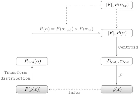
The statistical density modification techniques pioneered by Ter-williger (2004); Terwilliger and Berendzen (1999) and Cowtan (2000) are a different approach to reduce bias in DM. Rather than using a sin-gle modified map to express the a priori knowledge incorporated in the electron density map, statistical DM expresses the newly introduced in-formation in terms of probability distributions, which are subsequently carried forward into reciprocal space illustrated in Figure 1.10. Since the density-modified phase probabilities are no longer estimated from the agreement between the observed and density-modified structure fac-tor magnitudes, the link between the experimental and density-modified phase information is weakened.

Maximum likelihood allows for a rational incorporation of other sources of information. The use of maximum-likelihood in the phase-combination scheme described by Pannu et al. (1998) allows for incor-poration of experimentally determined phase information in the form of Hendrickson-Lattman coefficients. The method has been shown to out-perform theσAphase combination traditionally used in classical density modification (Cowtan 2010).

distri-|F|, P(αex)

|F|, P(α)

|Fbest|, αbest

ρ(x) P(ρ(x))

Pmod(α)

Centroid

F

Infer Transform

distribution

P(α) =P(αmod)×P(αex)

Figure 1.10: Steps in statistical density modification. Structure factor amplitudes and phases are indicated with|F|andα, respectively. Thea priori information inferred from the electron density, ρ(x) is expressed as probability distributions, P(ρ(x)). These are carried forward into reciprocal space, P(αmod) and multiplied with the experimental phase probabilities,P(αex) to obtain the updated phase probabilities, P(α).

1.3.4 Automated model building and refinement

Once the diffraction data is collected, manual model building and refine-ment of a protein structure are the single most time consuming tasks in solving a protein structure. Automatic chain tracing has made the over-all process of building a structural model of a protein substantiover-ally more efficient, which has benefited both high-throughput structure solution and structure solution in a non-automated setting. The computer pro-grams ARP/wARP (Langer et al. 2008), Resolve (Terwilliger 2000,

2002), Buccaneer (Cowtan2006) and SHELXE(Sheldrick 2002) are designed to build protein structures into electron density maps without user intervention. Although the implementation between the different programs differs, the basic premise is the same. Often the only input required is the amino acid sequence and a file with the structure fac-tor amplitudes and phases. In the first step towards model building the electron density map is populated with a number of seed atoms. Subsequently, the Cα _{atom seeds are connected into chain fragments} and individual amino acids or short peptides are docked into the frag-ments. The final stage often includes connecting the fragments into chains, building loops and resolving clashes.

To date theARP/wARPprogram is the most comprehensive solu-tion available, including high-level decision maker driven iterative tein model building, fast building of the secondary structure of a pro-tein, tracing of flexible loops in alternate conformations, fully automated placement of ligands, and locating ordered water molecules (Langer et al. 2008). The program initially required high resolution data (Perrakis et al. 1999), but later developments (Morris et al. 2002,2003) have re-laxed the resolution requirements and the recent inclusion of a secondary structure recognition routine allows partial model building down to 4.5 Å (Langer et al.2008).

is relatively simple and very suitable for incorporation into automation pipelines (Cowtan 2006). The method is reasonably fast and performs well on data of moderate to low resolution (Cowtan2006).

The programResolve carries out model building in somewhat dif-ferent, highly hierarchical fashion. Firstly, α-helices and β-sheets are located and fitted, followed by extension of these secondary structure elements with tripeptides, computed from a set of refined protein struc-tures. In the final stage individual fragments are connected into chains (Terwilliger 2002). In addition to performing model building Resolve includes a likelihood-based density modification procedure, that yields better phase improvement than conventional procedures such as solvent flattening and histogram matching (Terwilliger2000).

To improve a partial model and obtain the best electron density map, model building is often iterated with reciprocal space refinement. Ref-mac(Murshudov et al.2011) is a popular refinement program that uses different likelihood-based functions to best fit the experimental condi-tions and the availability ofprior information, for instance the presence experimental phase information in the form of a SAD or SIRAS signal. The various restraints and model parametrizations allow customization of Refmac to suit data quality. For instance, the use of secondary structure restraint or local and global NCS restraints can greatly ben-efit lower resolution data sets (Nicholls et al. 2012), whereas optional refinement of anisotropic B-factors can give the fullest description of a high resolution structure. The latter though is typically only used in the final stage of model refinement and not during the model (re)building stage.

Recent advances in

_Crank

Abstract

For its first release in 2004, Crank was shown to effectively

detect and phase anomalous scatterers from SAD data. Since then,

Crankhas significantly improved and many more structures can

be built automatically with single or multiple wavelength anoma-lous diffraction or SIRAS data. Here, we discuss the new algo-rithms we have developed that lead to the substantial improve-ments and show Crank’s performance on over one hundred real

data sets. The latest version ofCrankis freely available for

down-load athttp://www.bfsc.leidenuniv.nl/software/crank/and

from CCP4 (http://www.ccp4.ac.uk/).

The work in this chapter was published in N. S. Pannu, W.-J. Waterreus, P.

Skubák, I. Sikharulidze, J. P. Abrahams, and R. A. G. de Graaff (Apr. 2011). “Recent advances in the CRANK software suite for experimental phasing.” In:Acta Crystallographica, Section D: Biological Crystallography 67.Pt 4, pp. 331–7. doi:

10.1107/S0907444910052224

The author of this thesis implemented utilities for deployment of massive parallel tests on openPBS; implemented a generic framework for parsing log files and

au-tomated analysis of extracted statistics; performed minor debugging of theCrank

2.1

Introduction

Currently, many software packages are available to automatically solve structures. The main aim of Crank (Ness et al. 2004) is to provide a user friendly and automated system incorporating the latest computa-tional developments in all stages of structure solution by experimental phasing. Crankis not a monolithic system: users can define pipelines from a choice of many different programs. Figure 2.1shows the current steps that Crank can perform and the programs that users can select to perform the task. The externally developed programs that Crank can interface with areSHELXC(Sheldrick2008),SHELXD(Schneider and Sheldrick 2002), SHELXE (Sheldrick 2002), dm (Cowtan 1994), Parrot (Cowtan 2010), Pirate (Cowtan 2000), Buccaneer (Cow-tan2006),ARP/wARP(Langer et al.2008) both of which iterate with Refmac(Murshudov et al.2011) andResolve(Terwilliger2000,2002). We are the main authors of the programs Afro (Pannu et al., in preparation) for FA calculation, Crunch2 (de Graaff et al. 2001) for substructure detection, Bp3 (Pannu and Read 2004) for substructure phasing, Solomon (Abrahams and Leslie 1996) for density modifica-tion, Multicomb (Skubák et al. 2010) for phase combination and co-authors of the programRefmac. These programs use multivariate max-imum likelihood methods that allow the observed diffraction data and any current models to be considered simultaneously at any stage in the structure solution process. Thus, the wealth of information contained in the observed diffraction data can be used directly throughout the structure solution process and not approximated or ignored as current approaches do after constructing an initial electron density map.

Input: reflections

Substructure factor amplitude estimation

Afro,SHELXC

Substructure detection

Crunch2,SHELXD

Phasing

Bp3,SHELXE

Density modification

Solomon,Parrot, Pirate,Resolve

Model building (& refinement)

Buccaneer (& Refmac), ARP/wARP (& Refmac), Resolve

Output: model coordinates

The programs and methods we develop are not only available in Crank, but also AutoRickshaw (Panjikar et al. 2005) and ARP/wARP. Furthermore, the original methods we have developed have also been re-written in mathematically identical forms in both phenix.refine and phaser (Adams et al. 2010).

2.2

Recent developments in Crank

2.2.1 Substructure determination

After diffraction data has been indexed and merged, |FA| values are calculated for input to substructure detection programs. |FA| values are the amplitudes of structure factors corresponding to the heavy atoms to be located. For single-wavelength anomalous diffraction (SAD) data, most programs use the absolute value of Bijvoet differences, ∆F =||F+|−|F−||as an estimate for|FA|. Burla et al. (2002) proposed

employing multivariate joint probability distributions to obtain the ex-pected value for |FA| in an equation that contains three integrals. In

order to obtain an analytical solution to the integrals, Burla et al. (2002) assume the “Bijvoet phases” are equal. We have obtained an expression requiring only one numerical integration without making this assump-tion. This approach has been implemented in the program Afro and performs satisfactorily. Details of the implementation and test results will be shown elsewhere (Pannu et al., in preparation). The develop-ment version of Afro containing the multivariate |FA| calculation is available in the latest version of Crank and can be used as input for either Crunch2 orSHELXD.

of whether a correct substructure solution has been located: an option exists to run the substructure phasing programBp3 quickly in “check” mode and examine likelihood based statistics to determine whether a correct and complete substructure has been found. The statistic that Crankuses is a Luzzati (1952) parameter: if the average Luzzati param-eter is greater than a threshold value (the default is 0.7), it is assumed that the full substructure has been found and substructure detection is terminated. Using likelihood methods to validate substructure detection has been available in Crank for over three years (Pannu et al. 2007) and this approach has been appreciated by phenix developers, who re-cently adopted it in their own suite (Paul Adams, CCP4 bulletin board, 31 July 2010).

2.2.2 Substructure phasing

To incorporate anomalous phase information, heavy atom refinement programs such asSharp(Bricogne et al.2003) orMlphare (Collabora-tive Computational Project Number 41994; Otwinowski et al.1991) use a Gaussian function on observed Bijvoet differences (∆F =|F+| − |F−|)

centered on the “calculated” Bijvoet difference that is determined from an assumed value of the “true” structure factor and the heavy atom structure factor (Matthews 1966; North 1965). Since, in general, the “true” structure factor is not known for a SAD or multiple-wavelength anomalous diffraction (MAD) experiment,Sharpintegrates out the am-plitude and phase of the true structure factor. Furthermore,the estimate of measurement error for Bijvoet differences is determined by merging the measurement errors for Friedel pairs (σ_∆F =

q

σ_F2+ +σ_F2−), leading

to suboptimal use of experimental information.

To input the observed structure factors directly, it is necessary to consider a joint probability of all observations given a current model. We have previously shown that this method provides better results over other approaches for the case of SAD (Ness et al.2004; Pannu and Read

(Skubák et al.2009) which will be released in the next version ofCrank.

2.2.3 Density modification

In the density modification (DM) procedure, the density modified map is iteratively combined with the initial map obtained from experimental phasing. Current methods assume that these two maps are independent and propagate the initial map’s phase information indirectly through Hendrickson-Lattman coefficients (Hendrickson and Lattman1970). We have applied a multivariate analysis that considers the observed Friedel pairs directly for a SAD experiment, accounts for the correlation between the initial and density modified map and refines the errors that can occur in a SAD experiment. Results on many test cases show a significant improvement over the current state of the art (Skubák et al. 2010): the maps produced by the multivariate phase combination algorithm lead to many more structures being built automatically.

Despite the improvements in the quality of electron density maps, figures of merit remained escalated after DM. To obtain more accu-rate FOMs, we have recently developed and implemented a new cross-validated scheme for accurate error parameter estimation in likelihood based phase combination. The method leads to more reliable phase probability statistics from DM and results in a further improvement in subsequent model building. In addition, the more accurate FOMs en-able a more relien-able hand determination or identification of incorrect non-crystallographic symmetry (NCS) operators used in DM (Skubák and Pannu2011). These developments have been implemented in a new phase combination program calledMulticomband can be used in con-junction with either Solomon orParrot.

2.2.4 Automated model building and refinement

informa-tion via Hendrickson-Lattman coefficients (Hendrickson and Lattman

1970). Thus, the MLHL function is dependent on the accuracy and reli-ability of the coefficients that are input. Furthermore, in its derivation, the MLHL function assumes that the experimental phase information (represented by Hendrickson-Lattman coefficients) is independent from the calculated structure factor. This assumption is questionable, as the experimental phase information is used to build an initial model. To overcome these issues, we considered and derived a multivariate likeli-hood function for SAD (Skubák et al.2005) and SIRAS (Skubák et al.

2009) experiments. The likelihood functions take as input the diffraction data directly, the heavy atom coordinates and the calculated structure factors and accounts for correlation between them. Compared to the other likelihood functions inRefmac, more models are built automat-ically inARP/wARP with the multivariate functions. The SAD and SIRAS functions in Refmac are available in Crank both in model building withARP/wARP and Buccaneer.

2.2.5 Integration of programs and steps

To support the integration of the different programs it interfaces with, Crank has a plug-in architecture and communicates between plugins via an XML file. At the moment, there are two methods available to generate an XML file thatCrank uses to run a pipeline: the program gcx(Ness et al.2004) and aCCP4igraphical user interface. Both inter-faces toCrankcan be run with only minimal input: an mtz file with the relevant column labels specified, a sequence file and the name, expected number and f’ and f" values for the heavy atoms. However, users can cus-tomize settings for individual programs, define custom made pipelines using any programs at each step and define the start and end step for a particular pipeline.

Figure 2.2: Screenshot of the CCP4i GUIfor Crankshowing the few required fields and the possibility to customize pipelines for automatic stucture solution.

2.3

Methods

Here, we test the new methods described above on a wide range of real SAD, MAD and SIRAS merged diffraction data sets. For our tests, only the intensities or structure factor amplitudes, along with the sequence for a protein monomer, the number of substructure atoms expected per monomer and the f’ and f" values for the substructure atoms were input. Crank performed substructure detection using Afro and Crunch2,

Bp3for substructure phasing andSolomonwithMulticombwas used for DM. Three cycles ofBuccaneer iterated with Refmacwere used for automated model building with iterative refinement. All options or parameters were default in all programs. The defaults set by Crank depend upon the particular experiment: for SAD data,Afro uses the multivariate |FA| value calculation, Multicomb uses the multivariate SAD function for phase combination in DM while Buccaneer uses the SAD function implemented in Refmac. For SIRAS data, Afro calculates |FA| from either the anomalous signal or using isomorphous

differences by determining which signal is greater. Bp3 uses the un-correlated SIRAS function described previously (Pannu et al. 2003), Solomon uses MLHL phase combination inMulticomb, while

Buc-caneeruses the multivariate SIRAS function in Refmac. Finally, for MAD data, Afro chooses the wavelength with the greatest anoma-lous signal and calculates multivariate FA values from it. Similar to SIRAS data,Solomon uses MLHL phase combination inMulticomb to perform DM andBuccaneeruses the MLHL likelihood function in Refmacfor model refinement.

In the test cases below, the previous version ofCrank, 1.3, is tested with the current version, 1.4 The main differences between the two ver-sions is the development version of Afro that calculates multivariate

|FA|values given SAD data and the use ofMulticombfor phase com-bination in DM which are both introduced in version 1.4.

se-0 0.2 0.4 0.6 0.8 1 0

0.2 0.4 0.6 0.8 1

Fraction built Crank1.4

Fraction

built

Crank

1

.

3 _MAD

SAD SIRAS

Figure 2.3: Improvement of Crank version 1.4 compared with Crank version 1.3 in terms of the fraction of the model built for SAD, MAD and SIRAS data sets. The fraction of the model built is defined as the fraction of the coordinates that are within 1 Å of the coordinates of the structure deposited in the PDB.

lenium, sulfur, chloride, sulfate, manganese, bromide, calcium and zinc. Of the 116 data sets, 63 are MAD data sets, 46 are SAD data sets, and 7 are SIRAS data sets.

2.4

Results and Discussion

An example of an automatically built structure with a weak signal is GerE (Ducros et al.2001). The structure of GerE was originally solved with a four wavelength seleno-methionine MAD data set collected at 2.7 Å and a native data set diffracting to 2.1 Å. Crank version 1.3 could build the structure from just the peak data set to a high degree, but failed to build the structure with just the SAD inflection data set. Crankversion 1.4 can build the structure to a high degree using either the peak or inflection data set. We are unaware of any other automated package or collection of algorithms that can build GerE using either the peak or inflection data set automatically. To give an indication of the anomalous signal, Figure2.4plots the Bijvoet ratio (i.e. |∆F|

|F| ) as a function of resolution bin for the GerE peak and inflection wavelength data: the overall Bijvoet ratios for the peak and inflection data are 0.167 and 0.139, respectively.

For the 77 structures that were built automatically, substructure determination successfully terminated early in 69 of the cases. For 33 of the 69 cases, the Luzzati parameter statistics inBp3 allowed the early termination, while the remaining 36 cases the complete substructure was validated by an analysis of theCrunch2statistics.

2.4.1 Analysis of data sets that were not automatically built

39 of the 116 data sets could not be built automatically by Crank. 19 of the 39 data sets failed at substructure detection and could be built automatically if the resolution cutoff inCrunch2was changed or SHELXCandSHELXDwas used in substructure detection. It should also be noted that the five cases that could not be built in version 1.4 but were successful in version 1.3 are all due to the changes in the substructure detection algorithm. These tests will be used to further debug and improve the development version of the multivariate |FA|

calculation inAfro.

3 4 5 6 7 8 9 10 6·10−2

8·10−2 0.1 0.12 0.14 0.16 0.18 0.2 0.22 0.24

Resolution Å

Bijv

oet

ratio

Peak Inflection

Figure 2.4: Plot of the Bijvoet ratios as a function of resolution for the peak and inflection wavelength data of the GerE test case. The peak and inflection wavelength are shown with a solid and dashed line, respectively.

function in Bp3had failed to produce an automatically traceable map. The multivariate SIRAS function for phasing will be released in the next version of Crank.

be determined.

2.5

Conclusions and future developments

Because of the new methods we have developed,Crankcan build many more structures automatically and can build structures where current methods fail. Crank’s robustness is shown by the large number of data sets we use in this test that require very minimal input.

Crank’sCCP4i GUIis easy to use, but does have some limitations. Firstly, log files are only updated once a particular step in the pipeline has finished. Secondly, users can not manually stop a current step and proceed to a next step. Instead the pipeline can only be terminated and the Crank run must be restarted from the beginning. Furthermore, although, Crank has an interface to Coot (Emsley et al. 2010), it cannot show real time updates of a model as a Crank run proceeds. All of these shortcomings are being addressed and a new pyQt (http:// www.riverbankcomputing.co.uk/software/pyqt/intro) interface for

Crankis currently being developed in collaboration with CCP4. Although having an easy to use and powerful interface is important, the first priority for Crank will always be developing better methods to solve data sets that elude current methods. For the case of MAD data, current approaches in Crank and elsewhere use univariate, un-correlated likelihood functions forFAcalculation, substructure phasing and the MLHL function for DM and automated model building and re-finement. Obviously, a multivariate MAD function could address the shortcomings in current approaches and could lead to structures where current methods fail.

A new method for phase combination

Abstract

DM is a standard technique in macromolecular crystallogra-phy that can significantly improve an initial electron density map. To obtain optimal results, the initial and density modified map are combined. Current methods assume these two maps are indepen-dent and propagate the initial map information and its accuracy indirectly through previously determined coefficients. We have derived a multivariate equation that no longer assumes indepen-dence between the initial and density modified map, considers the observed diffraction data directly, and refines the errors that can occur in a single wavelength anomalous diffraction experiment. We have implemented and tested the equation on over one hun-dred real data sets. Results are dramatic: the method provides significantly improved maps over the current state of the art and leads to many more structures built automatically.

The work in this chapter was published in P. Skubák, W.-J. Waterreus, and N. S. Pannu (June 2010). “Multivariate phase combination improves automated crystallographic model building”. In:Acta Crystallographica, Section D: Biological Crystallography66.7, pp. 783–788.doi:10.1107/S0907444910014642∗The first two authors contributed equally.

The author of this thesis implemented utilities for deployment of massive parallel tests on openPBS; implemented a generic framework for parsing log files and automated