SPATIAL AND TEMPORAL SCALING OF NITROGEN CYCLING AND EXPORT: RESOLVING THREE PARADOXES FOR A FORESTED PIEDMONT WATERSHED
Jonathan Macdougal Duncan
A dissertation submitted to the faculty of the University of North Carolina at Chapel Hill in partial fulfillment of the requirements for the degree of Doctorate of Philosophy in the Department of Geography.
Chapel Hill 2014
Approved by: Lawrence E. Band Emily Bernhardt
Martin Doyle Peter Groffman
©2014
ABSTRACT
Jonathan M Duncan: Spatial and Temporal Scaling of Nitrogen Cycling and Export: Resolving Three Paradoxes for a Forested Piedmont Watershed
(Under the direction of Lawrence E. Band)
Nitrogen is a limiting nutrient in many forest and aquatic ecosystems. Reducing nutrient pollution to downstream receiving waters is an important scientific and management goal. Disproportionate amounts of nitrogen cycling and export occur in small portions of the landscape and over brief periods of time. These “hot spots” and “hot moments” are highly heterogeneous in space and time, making scaling of nitrogen cycling and export a major scientific challenge. This dissertation addresses how linkages between the physical structure of a watershed and related hydrological, ecological, and biogeochemical
processes control the spatial and temporal patterns of nitrogen cycling and export. This work was conducted at Pond Branch, a small, forested watershed in the Piedmont physiographic province in Maryland (USA). This dissertation has three related multi-scale questions that are addressed by employing three different views of watershed ecohydrology (plan view, cross sectional, and longitudinal). Detailed observations and analysis at Pond Branch suggest that the ecohydrological processes in the riparian zone (which accounts for 4% of the catchment area) control nitrogen cycling and export at the watershed scale. In particular:
on the timing and magnitude of nitrogen export as shown in evolving concentration-discharge relationships.
ACKNOWLEDGEMENTS
I have MANY people to thank for helping me accomplish what is contained within this dissertation and many more to thank for accomplishments not within the following pages. From diligent librarians, sensor and datalogger technical support staff, to colleagues and peers throughout formative stages of this work there has been a large number of people that assisted in small but important ways. I also acknowledge the giants in the fields of geomorphology (Reds Wolman), biogeochemistry (Gene Likens and Herb Bormann), and watershed science (Pat Mulholland), on whose shoulders I’ve been standing.
The help and friendship of lab mates and departmental friends including Yuri Kim, Charles Scaife, Monica Smith, Tamara Mittman, Daisy Small, Autumn Thoyre, and especially Taehee Hwang, Brian Miles, Josh Gray, and Jeff Muelhbauer has been immeasurable. I’ve been lucky to have lots of help in the field. My old friend Steve Berkstresser whose life’s circumstances brought him to Baltimore, MD helped with the logistics of frequent trips to Baltimore and helped with the occasional lugging of
equipment when I couldn’t. Dan Jones, Gray Redding, Nate Moore, Samantha Forester, and in particular Dan Dillon have been instrumental in making this dissertation happen. Dan’s friendship and flexible nature have helped this research. Claire Welty and the CUERE staff have also helped with some travel logistics, funds and GPS work. Brooke Hassett in the Bernhardt lab had the patience and expertise to help me get reacquainted with lab procedures and water quality analysis. Jack Weiss’s statistical help and R tutoring have been instrumental in these results. His quick, thorough, and accurate explanations are greatly appreciated.
free me of epistemological confirmation biases and see the stream as an ecosystem. Her wit and wisdom, humor and humanity have helped improve this dissertation in substantial ways. Martin Doyle has been helpful in realms and roles ranging from armchair
philosopher to life coach to academic mentor. Martin has helped me see the streambed as highly dynamic and has encouraged me to “go all Schumm and Lichty” on things with reckless abandon. Peter Groffman has worked very closely with me throughout this dissertation. I am truly thankful to have Peter on my committee. His endless enthusiasm, in-depth and quick reviews with an always-impressive mix of constructive, optimistic, and humorous comments have helped me see the big picture on many occasions. There need to be more people like Peter in this world, especially in academia. And most importantly, I acknowledge my advisor Larry Band. In fact, Larry has been much more than an advisor to me. He is a mentor and a role model. I couldn’t imagine a better person to have helped me through this process. His breadth and depth of knowledge, patience, kindness, and unwavering academic support are unparalleled. He has given me the freedom to think deeply about the bigger questions rather than quickly write up the low hanging fruit. His version of academia is the one I ascribe to. I will judge my career a smashing success if I can help a future researcher as Larry has helped me.
And finally to my beautiful and exceptionally supportive wife and children: The hours I spend with them are the brightest of my day. Ben has been there throughout my PhD to give me the best perspective on what’s really important in life. He’s been there to ‘help’ in the field and to say how cool my figures are at home. When she’s not wrapping me around her precious little fingers, Cassidy has given me the push to get this dissertation done. Given the time spent away from them to work on this is, I hope its completion can make them proud some day. And most importantly, to my best friend, my dearest
Heather: She knew I wanted to get back into research and despite knowing that it
required giving up the very comfortable life we had in Washington, she encouraged me to go back for a PhD and pursue my dreams. She’s been there through thick and thin,
TABLE OF CONTENTS
LIST OF FIGURES ... x
LIST OF TABLES ... xiii
CHAPTER 1. INTRODUCTION ... 1
CHAPTER 2: TOWARDS CLOSING THE WATERSHED NITROGEN BUDGET: SPATIAL AND TEMPORAL SCALING
OF DENITRIFICATION ... 22
CHAPTER 3: ECOHYDROLOGIC CONTROLS OF SEASONAL NITRATE
EXPORT IN A FORESTED HEADWATER CATCHMENT ... 63
CHAPTER 4. RIPARIAN ECOHYDROLOGIC CONTROLS ON PATTERNS
OF STREAM NITRATE EXPORT ... 108
LIST OF FIGURES
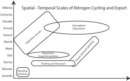
Figure 1.1 Characteristic space-time scales for biogeochemical processes ... 12
Figure 1.2 Simplified version of the nitrogen cycle. ... 13
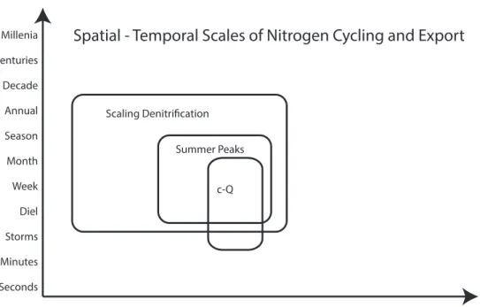
Figure 1.3 Spatial and temporal template for dissertation chapters. ... 13
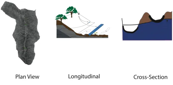
Figure 1.4. Three views of watershed ecohydrology presented in this dissertation. ... 14
Figure 2.1. LiDAR derived shaded relief image of the Pond Branch watershed ... 52
Figure 2.2. Upper and Lower Riparian Transect cross-sections with sensor locations ... 53
Figure 2.3. Topographic Wetness Index of the Pond Branch watershed. ... 54
Figure 2.4. Riparian hummock and hollow delineation near the upper riparian transect computed from TWI thresholds ... 55
Figure 2.5. The percent of riparian pixels defined as a hollow based on varying thresholds of topographic wetness index values ... 56
Figure 2.6. Soil oxygen concentrations for different landscape positions for WY 2011 at each of the three data logger locations ... 57
Figure 2.7. Cumulative percent oxygen plots for riparian hollow, toeslope and hillslope hummock landscape positions. ... 58
Figure 2.8. N2 fluxes in soil cores from upland, hillslope hollow, riparian hummock and riparian hollow landscape positions ... 59
Figure 2.9. N20 fluxes in soil cores from upland, hillslope hollow, riparian hummock and riparian hollow landscape positions ... 60
Figure 2.10. Model of daily N2 flux for riparian hollow, toeslope and hillslope hollow landscape positions ... 61
Figure 2.11. Scalar model of net nitrification-denitrification as a function of soil moisture for sandy loam soils ... 62
Figure 3.1. Conceptual model of summer season nitrate sources. ... 97
Figure 3.2. LiDAR derived shaded relief image of the Pond Branch watershed ... 98
Pond Branch bottomland. ... 99
Figure 3.4. Bi-weekly NO3 concentrations from weekly BES grab samples ... 100
Figure 3.5. Longitudinal stream samples ... 101
Figure 3.6. Nitrate concentrations collected at a groundwater seep and the outlet ... 102
Figure 3.7 Stream nitrate and stage measurements at 15-minute resolution over a 4 day period at baseflow ... 103
Figure 3.8. Nitrate concentrations versus day of year in 2010- 2011 in tension lysimeters in riparian and upland locations in the Pond Branch watershed ... 104
Figure 3.9. Average daily soil oxygen concentrations measured in toeslope, riparian hummock, and riparian hollow landscape positions Dec 18, 2011 – Oct 11, 2012 ... 105
Figure 3.10. Soil oxygen concentrations measured hourly in toeslope, riparian hummock, and riparian hollow landscape positions from June 18 – July 8, 2011 ... 106
Figure 3.11. A conceptual model of how seasonal and diel (transpiration-induced) water table fluctuations provide the biogeochemical conditions to produce and transport nitrate from the riparian zone to the stream during the growing season ... 107
Figure 4.1. Map of Pond Branch watershed, MD within the larger Baisman Run Watershed ... 130
Figure 4.2. Locally weighted regression (LOESS) fit of nitrate-N concentrations (mg/L) for each year (1998 – 2012) based on weekly grab samples. ... 131
Figure 4.3. High resolution nitrate concentration data from 2011 in relation to long-term weekly grab sample concentrations and long-term LOESS fit. ... 132
Figure 4.4. Discharge, nitrate concentrations, and mass flux from June 22 – 26, 2011; an ascending limb that accounted for the majority of the seasonal increase in nitrate concentration and flux for the year. ... 133
Figure 4.5. Soil oxygen concentrations in toeslope, riparian hummock and riparian hollow landscape positions from June 20 – July 6, 2011. ... 134
Figure 4.7. High resolution nitrate concentration versus discharge from
June 20 – 26, 2011. ... 136
Figure 4.8. High resolution nitrate concentration versus stage from
July 13 - 20, 2011. ... 137 Figure 4.9. High resolution nitrate concentration versus stage from
July 29 – August 10, 2011. ... 138
Figure 4.10. High resolution nitrate concentration versus stage from
September 18 - 27, 2011. ... 139 Figure 4.11. A new conceptual model for controls of stream
nitrate concentrations. ... 140
Figure 5.1 Hydroclimate (precipitation and temperature) and nitrogen deposition inputs are filtered through the
LIST OF TABLES
Table 2.1. Denitrification N2 fluxes, soil nitrate concentrations, in situ and potential net N mineralization and nitrification, and microbial
respiration from cores collected from seven different landscape positions ... 49
Table 2.2. Equations relating denitrification N2 flux and incubation O2 levels ... 50
Table 2.3. Nitrogen inputs and outputs for the Pond Branch watershed for WY 2011 ... 51
Table 3.1. Mean Monthly Discharge at Pond Branch through the growing season ... 96
Table 5.1 Watershed Scale Nitrogen Mass Balance ... 155
CHAPTER 1. INTRODUCTION
Understanding the spatial and temporal heterogeneity of hydrological and
biogeochemical controls on nitrogen cycling and export is a major scientific challenge (Lohse et al., 2009). The heterogeneity in hydrological and biogeochemical processes are themselves controlled by the watershed geomorphology and the variability of the
geomorphic template. Stream water quality and quantity are integrated signals of different catchment hydrological and biogeochemical mechanisms, source areas, and flowpaths, all of which are highly nonlinear and can change over time. Changes can occur on timescales ranging from individual storm events to multiple years. My goal is to better understand the mechanisms by which forested watersheds retain and export water and nitrogen. This requires understanding the spatiotemporal variability in complex and interdependent processes. Hydrologic controls on these processes include groundwater levels, soil moisture content, connectivity, and residence times along flowpaths. These processes have characteristic space-time scales that can be useful for hydrological
modeling (Blöschl and Sivapalan, 1995). Understanding nitrogen cycling and export also requires knowing the biogeochemical controls along these flowpaths. Biogeochemical controls of terrestrial nitrogen cycling include microbially-mediated transformations that are functions of energy (labile carbon), reactant concentrations, and soil oxygen,
moisture, and temperature ranges. Because each of these controls is highly variable in space and time (Figure 1.1), it is important to develop appropriate measurements and models that account for this heterogeneity.
General Background Nitrogen Cycle
The major biological nitrogen cycle processes in a forested watershed include the following: (Figure 1.2):
• Biological fixation- conversion of dinitrogen gas to ammonia • Assimilation- Incorporation of inorganic nitrogen into amino acids • Mineralization/Ammonification- production of ammonia by microbial
decomposition
• Nitrification- aerobic production of nitrate from ammonium
• Denitrification- anaerobic reduction of nitrate to nitrous oxide and dinitrogen gas Less common biological processes include:
• Dissimililatory nitrate reduction to ammonium (DNRA)- anaerobic conversion of nitrate to ammonia
• Anammox- anaerobic ammonium oxidation of nitrate produces dinitrogen gas
Physical processes include:
• Sorption and desorption – physical process of binding between bulk phase (liquid or gas) and a surface (soil)
• Volatilization- ammonia gas lost from soil to the atmosphere
My work considers the major biological processes, other processes may warrant further investigation in future research at Pond Branch.
Hydrologic controls
Groundwater levels have been found to be a primary control on nitrogen cycling and dynamics in riparian zones (Hefting et al., 2004). Hefting et al. found that across a set of European catchments with average water tables within 10cm of the soil surface,
below 30cm, nitrate accumulates as a result of nitrification. Less work has been done to assess if and how water table fluctuations within a watershed control nitrogen cycling. Soil moisture is the result of interactions among climate, vegetation, and soil and is an important controlling factor of nutrient cycling (Pastor and Post, 1986). Soil moisture can be an important driver of soil oxygen levels, plant nutrient uptake and water stress, and for sustaining microbial communities. Variations in soil moisture at the plot scale could enable coupled denitrification and nitrification. Nitrification could occur during drier oxygenated conditions and denitrification would occur when oxygen levels drop. Coupled nitrification and denitrification is especially plausible when nitrate availability limits denitrification. There is a lack of research on coupled nitrification-denitrification as a result of soil moisture variability.
At landscape scales, the geographic patterns of soil moisture are related to the hydrologic connectivity of a catchment (Western et al., 1997; James and Roulet, 2007) . Topography is an important control on soil moisture distributions, especially in non-storm periods or more humid catchments. Topography can also determine the strength of connectivity between hillslopes, riparian zones, and streams (Jencso et al., 2009). Highly connected portions of a watershed can receive or contribute disproportionate amounts of
throughflow or groundwater to riparian zones and streams. Many studies have noted the particular importance of riparian zones in controlling denitrification and potentially determining streamflow chemistry (Bishop et al., 2004).
Residence time distributions along flowpaths are an important control on
Biogeochemical controls
Biogeochemical controls on nitrogen cycling are complex and highly variable in space and time. Reaction rates are dependent upon a combination of microbial, plant, and environmental factors.
Environmental and soil factors are important controls on nitrogen cycling rates. Soil moisture and temperature drive the activity of microbial respiration (Pastor and Post, 1986); (Parton et al., 1996). Soil structure and texture can control how long soil water is available to microbes and the amount of microsites for reactions to take place. Perhaps the most important environmental control is soil oxygen levels, which have considerable control over the rates of nitrification, denitrification, and ammonification (Reddy and Patrick, 1975) (Hedin et al., 1998; Hill, 1996). Oxidation and reduction (redox) reactions are especially important processes that regulate nutrient cycling. Oxic vs. anoxic conditions have been viewed as thresholds for nitrification and denitrification reactions, but recent work has shown that these processes are coupled in many soil environments. Soil oxygen sensors in surficial soils were used to obtain a high temporal resolution dataset and determine the duration and magnitude of anoxic conditions.
Reactant availability (nitrate for denitrification or ammonium for nitrification) is
typically a controlling factor (Groffman et al., 2009). These reactants can be produced in situ or transported from upslope areas. In the absence of input or transformation, a given patch of soil will quickly become substrate limited. For example, denitrification in an anoxic region with in situ supplies of nitrate exhausted could only occur through production of new nitrate in the presence of variation in oxygen levels or transport of nitrate from connected patches. Introducing oxygen variability could produce nitrate via nitrification, then revert back to anoxic conditions for denitrification to proceed.
Secondly, precipitation-driven advection or some other sort of nitrate addition (e.g., fertilization, deposition) could also stimulate denitrification.
Microbial community composition is an important control on nitrogen cycling.
et al., 2006). Rapid fluctuations in redox potential have also been found to alter
community structure (DeAngelis et al., 2010). Anaerobic heterotrophs can alter element cycles by reducing nitrate, iron, manganese, and sulfur.
An energy source for microbial respiration is also necessary. This is typically in the form of labile carbon, but other compounds such as reduced sulfur, reduced iron, or methane can be used. Laboratory measures of microbial respiration were used as a surrogate for carbon availability.
Vegetation can play an important role in the cycling of nitrogen. Different plant species have distinct carbon to nitrogen ratios. The leaves then impart that signature into litter. C:N ratios can effect how quickly nutrients are cycled, mineralization and nitrification rates, and how much is available for hydrologic transport (Lovett et al., 2004).
Geomorphic controls
The physical structure of a watershed imparts a fundamental control on where, when, and how long parts of the landscape can transmit, collect, and drain water. There are long-term feedbacks among the pedogenesis, climate drivers which include precipitation and evapotranspiration, and vegetation. Landscape topography and landscape position has long been seen an import control for hydrology and biogeochemistry (Gregory and Walling). The presence of riparian zones and frequently saturated areas such as
hillslope hollows are directly related to the frequency of advection of water and solutes. To an extent larger scale land forms co-evolve with vegetation and climate and set the stage for subsequent biogeochemical reactions. Additionally, the microscale
geomorphic template of watersheds is an important control for redox sensitive biogeochemical transformations.
Human Alteration of the N cycle
amount of reactive nitrogen globally by nearly two orders of magnitude from pre-industrial background levels (Galloway, 2003). Over the last century, there has been a corresponding and dramatic increase in N loading to receiving waters around the globe. Even N export from forests where N retention is relatively high is a significant fraction of overall stream flux. In the Chesapeake Bay, the largest estuary in the country, nearly 20% of the total nitrogen load is estimated to come from forests, despite comprising ~ 55% of the watershed area (Jantz et al., 2005).
There is great interest in the ability of forests to serve as “sinks” for atmospheric N, especially when excess N can stimulate primary production in estuaries which can then lead to widespread anoxic zones (Boesch et al. 2001, Conely et al. 2009). Understanding the mechanisms of how ecosystems serve as N sinks through assimilation, storage and denitrification is especially important given the changing spatial and temporal
distributions of N sources and trnsport vectors including: a) restoration strategies and watershed management plans which attempt to restore the form and function of forests), and b) the periods of time that transport and transform disproportionately high amounts of N (hot moments) could be altered by the changing climate. As temperatures increase, there could be higher rates of evapotranspiration and lower water tables leading to a decrease in denitrification. Additionally, there is mounting evidence for changes in the frequency of rainfall (Chou et al., 2012) including longer times between storms, and an increase in the intensity of extreme rainfall events (Westra et al., 2013).
Spatial and temporal scales of variability of hydrological and biogeochemical controls
Variability of hydrological and biogeochemical drivers can exist at all temporal and spatial scales. Disproportionate amounts of nitrogen can be transformed or transported during brief periods of time (hot moments) in discrete patches of the landscape (hot spots) (McClain et al., 2003). Because there are many intertwined controls,
Temporal variability of hydrological and biogeochemical controls can be very high at all time scales. At inter-annual scales, there are climatic differences in dry and wet years. Longer timescale variability may also relate to disturbance of ecosystem growth and succession (Aber et al., 1997; Schimel et al., 1996). There are profound differences in nitrogen cycling and export dynamics at seasonal timescales driven by forest cycles. Rates and fluxes can differ markedly between winter and summer months (Miller et al., 2009). In temperate forests, leaf senescence can dramatically increase labile carbon supplies and fuel denitrification (Groffman and Tiedje, 1989; Sebestyen et al., 2008). Plant uptake is typically highest during the summer growth months and lowest during leaf-off (Stoddard, 1994). Causes and sources of diurnal streamflow have been examined for more than 60 years (Troxell, 1936) and have been a recent focus for hydrologic (Bond et al., 2002; Wondzell et al., 2007) and biogeochemical (Rusjan and Mikoš, 2010) research. Episodic events such as rainfall events transport carbon and nitrogen to hot spots where microbial transformations occur. Event sampling of water, carbon, and nitrogen has been the focus of several studies revealing the importance of variable source areas (Inamdar et al., 2004) and groundwater seeps (Burns et al., 1998).
Spatial variability of hydrological and biogeochemical drivers can be highly
heterogeneous from watershed to microsite scales. At the catchment scale, the major spatial differences fall out along different landscape positions. In temperate forests, ridges, hillslope hollows, and riparian areas exhibit different frequencies of wetting. Understanding the extent and duration of wetting in these different topographic settings is also important for determining nitrogen cycling and export rates.
Variability and transport: plot and catchment scale hotspots
Accounting for both hydrologic variability and transport is required for understanding nitrogen cycling and export. Variability in hydrological and biogeochemical drivers is common at the plot scale on diurnal cycles or across space. Part of this dissertation investigates the integrated water table-soil oxygen condition across a range of
hydrologic regimes, include baseflow, typically considered a cold moment. In response to diurnal variations of soil moisture and oxygen, nitrification can proceed in aerobic environments producing nitrate for denitrification to occur when oxygen levels drop. Anoxic environments could occur in response to nightly decreases in soil oxygen values. In addition to within plot variations, there are larger differences among plots in different landscape positions. This reflects the geomorphic structure of watersheds and relates to the frequency of hydrologic flushing through different parts of the landscape. Catchment scale hotspots relate to the topography and connectivity that develops during
precipitation events and seasonal timescales. Considering plot and catchment scale variability is essential for adequate understanding.
Major Questions and Organization the Dissertation:
This dissertation seeks to advance understanding of nitrogen cycling and export by using distributed measurements and models to scale from cores to the catchment and from minutes to more than a decade. I examine the heterogeneity in water and nitrogen
dynamics across a range of spatial and temporal scales in each chapter (Figure 1.3). This work was conducted in Pond Branch, a small, forested watershed in the Piedmont
physiographic province in Maryland (USA). The sequence of individual chapters that address these multiscale puzzles are arranged along three major ways to view a catchment (sensu Leopold, 1994): 1) catchment and landscape scale in plan view, 2) longitudinal profile from highest and furthest point in the catchment, down the stream to the outlet, and 3) a cross section from western most ridge to eastern-most ridge, with a focus on the stream and near-stream zone (Figure 1.4).
Chapter 2 explores how nitrogen cycling regimes change in different landscape positions across seasons and develops a catchment scale denitrification estimate for an entire water year. In many forested catchments, despite large amounts of atmospheric N deposition, there are surprisingly high rates of retention. So, where does all the N go (van Breeman et al., 2002)? The focus of resolving this paradox at Pond Branch was to examine hot spots and hot moments of denitrification and scale denitrification estimates from cores to the catchment. A leading hypothesis is that most sampling and modeling approaches do not properly account for hydrologic processes in both space and time, and may miss a substantial amount of denitrification, the conversion of reactive nitrate and nitrite to nitrogen gases (nitric oxide, nitrous oxide, dinitrogen) (Kulkarni et al, 2008).
Chapter 3 investigates the role of diurnal fluctuations in riparian groundwater, soil moisture, and soil oxygen on summer peaks in streamwater nitrogen concentrations. Paradoxically, the majority of nitrate is exported via the stream at Pond Branch during the summer when the ecosystem should be taking it up. Unlike at some other
watersheds- groundwater is depleted in nitrate relative to the stream. Even if the source of summer nitrate is temperature driven mineralization and nitrification, which also peaks in summer- there is still a hydrological puzzle as the geographic sources of nitrate are surface soil- not a region that contributes to baseflow. One of the greatest challenges in watershed science is understanding how the cumulative effects of ecosystem and hydrologic processes occurring throughout terrestrial and in-stream flowpaths
Chapter 4 uses high-resolution concentration-discharge (c-Q) relationships to examine the evolution of c-Q patterns at storm to seasonal timescales. The paradox in this chapter is that nitrate c-Q patterns are different between those generated by long-term weekly grab samples and storm based c-Q in many other forested watersheds (Inamdar et al., 2004, Sebestyen et. al, 2009). Understanding how multiple processes occurring over different temporal and spatial scales control c-Q patterns is important for understanding how much nitrate will be exported during storm events and over the longer timescales.
Significance of Dissertation Scientific importance:
Controls on watershed nitrogen cycling are complex and multi-scale. Linking and integrating ecohydrologic processes across scales is a major scientific challenge (Baird and Wilby, 1999). Nitrogen biogeochemistry is an interesting theoretical example because of numerous nonlinearities that are mediated by biological and hydrological processes. Considering that a disproportionate amount of nitrogen cycling occurs in small portions of a soil core (Parkin, 1987) and small portions of a catchment (McClain et al., 2003), addressing larger scale (regional and river-basin) issues of nitrogen pollution requires improved understanding of controls across scales. A second scientific challenge is the ability to predict N cycling and export in unmonitored locations. Part of this
Societal importance:
Altering when and where N transformations and transport will occur requires a more comprehensive understanding that can be operationalized in different watersheds. A major goal of watershed management and pollution mitigation programs such as the total maximum daily load (TMDL) program is to ‘restore’ watershed form and function of disturbed watersheds towards that of forested watersheds. This typically involves trying to reconstruct the function of hot spots and hot moments. Developing resilient
management strategies that can provide retention and removal of reactive N have challenges in the spatial optimization of management strategies at a range of scales. Ecosystem services of N removal/retention may occur primarily as denitrification from hot spots and hot moments. The research presented here contributes to the following N management issues:
1. Critical Loads for atmospheric N deposition have been used to quantify soil and stream export thresholds, but depend heavily on the ability for a given watershed to retain, transform, and transport N loads.
2. Spatial optimization of watershed management practices is critical for efficient expenditures of limited resources.
3. Stream restoration and afforestation efforts aimed at restoring the ecosystem form also need to restore ecosystem function.
We note that N export at Pond Branch is very low and similar forest catchments are not a major N source to the Chesapeake Bay. However, this research can be put in the context of pollution sources and management approaches to improve ecosystem retention in other landscapes. The hope is that better understanding of the relationship between the
Figure 1.1 Characteristic space-time scales for biogeochemical processes. Pore Core Patch Catena Position
(Landscape)Catchment Physiographic Continent Planet Seconds
Minutes Millenia
Centuries
Storms Diel Week Month Season Decade
Annual
Spatial - Temporal Scales of Nitrogen Cycling and Export
Atmospheric Depostition
Respiration Evapotranspiration Vegeta
tion Gr owth
Flushing and Transport
Microbial Dynamics
Stream Net work Spir
Figure 1.2 Simplified version of the nitrogen cycle. Adapted from (Trimmer et al., 2003)
Figure 1.3 Spatial and temporal template for dissertation chapters. Scaling Denitification (Chapter 2), Summer Peaks (Chapter 3), and concentration-discharge (c-Q) patterns in Chapter 4.
Pore Core Patch Catena Position Catchment Physiographic Continent Planet
Seconds Minutes Millenia
Centuries
Storms Diel Week Month Season Decade
Annual
c-Q Summer Peaks Scaling Denitrification
REFERENCES
Aber, J. D., S. V. Ollinger, and C. T. Driscoll (1997), Modeling nitrogen saturation in forest ecosystems in response to land use and atmospheric deposition, Ecological Modelling, 101(1), 61-78.
Band, L. E., C. L. Tague, P. M. Groffman, and K. Belt (2001), Forest ecosystem
processes at the watershed scale: hydrological and ecological controls of nitrogen export., Hydrological Processes, 15(10), 2013-2028.
Bernhardt, E. S., et al. (2005), Can't See the Forest for the Stream? In-stream Processing and Terrestrial Nitrogen Exports, BioScience, 55(3), 219-230.
Bishop, K., J. Seibert, S. Köhler, and H. Laudon (2004), Resolving the Double Paradox of rapidly mobilized old water with highly variable responses in runoff chemistry, Hydrological Processes, 18(1), 185-189.
Blöschl, G., and M. Sivapalan (1995), Scale issues in hydrological modelling: A review, Hydrological Processes, 9(3-4), 251-290.
Bond, B. J., J. A. Jones, G. Moore, N. Phillips, D. Post, and J. J. McDonnell (2002), The zone of vegetation influence on baseflow revealed by diel patterns of streamflow and vegetation water use in a headwater basin., Hydrological Processes, 16, 1671-1677.
Boyer, E. W., R. B. Alexander, W. J. Parton, C. Li, K. Butterbach-Bahl, S. D. Donner, R. W. Skaggs, and S. J. D. Grosso (2006), Modeling Denitrification in Terrestrial and Aquatic Ecosystems at Regional Scales, Ecological Applications, 16(6), 2123-2142.
Burgin, A. J., P. M. Groffman, and D. N. Lewis (2010), Factors Regulating Denitrification in a Riparian Wetland, Soil Sci. Soc. Am. J., 74(5), 1826-1833.
Cleaves, E. T., A. E. Godfrey, and O. P. Bricker (1970), Geochemical Balance of a Small Watershed and Its Geomorphic Implications Geological Society of America Bulletin, 81(10), 3015-3032.
Creed, I. F., and L. E. Band (1998), Exploring functional similarity in the export of nitrate-N from forested catchments: A mechanistic modeling approach, Water Resources Research, 34(11), 3079-3093.
DeAngelis, K. M., W. L. Silver, A. W. Thompson, and M. K. Firestone (2010), Microbial communities acclimate to recurring changes in soil redox potential status, Environmental Microbiology, 12(12), 3137-3149.
Detty, J. M., and K. J. McGuire (2010), Threshold changes in storm runoff generation at a till-mantled headwater catchment, Water Resour. Res., 46(7), W07525.
Goodale, C., S. Thomas, G. Fredriksen, E. Elliott, K. Flinn, T. Butler, and M. Walter (2009), Unusual seasonal patterns and inferred processes of nitrogen retention in forested headwaters of the Upper Susquehanna River, Biogeochemistry, 93(3), 197-218.
Gregory, K. J., & Walling, D. E. (1976). Drainage basin form and process: A geomorphological approach.
Groffman, P., K. Butterbach-Bahl, R. Fulweiler, A. Gold, J. Morse, E. Stander, C. Tague, C. Tonitto, and P. Vidon (2009), Challenges to incorporating spatially and temporally explicit phenomena (hotspots and hot moments) in denitrification models,
Groffman, P. M., and J. M. Tiedje (1989), Denitrification in north temperate forest soils: Spatial and temporal patterns at the landscape and seasonal scales, Soil Biology and Biochemistry, 21(5), 613-620.
Groffman, P. M., N. J. Boulware, W. C. Zipperer, R. V. Pouyat, L. E. Band, and M. F.
Colosimo (2002), Soil Nitrogen Cycle Processes in Urban Riparian Zones, Environmental Science and Technology, 36(21), 4547-4552.
Groffman, P. M., M. A. Altabet, J. K. Böhlke, K. Butterbach-Bahl, M. B. David, M. K. Firestone, A. E. Giblin, T. M. Kana, L. P. Nielsen, and M. A. Voytek (2006), METHODS FOR MEASURING DENITRIFICATION: DIVERSE APPROACHES TO A
DIFFICULT PROBLEM, Ecological Applications, 16(6), 2091-2122.
Haga, H., Y. Matsumoto, J. Matsutani, M. Fujita, K. Nishida, and Y. Sakamoto (2005), Flow paths, rainfall properties, and antecedent soil moisture controlling lags to peak discharge in a granitic unchanneled catchment, Water Resour. Res., 41.
Hedin, L. O., J. von Fischer, N. E. Ostrum, B. P. Kennedy, M. G. Brown, and G. P. Robertson (1998), Thermodynamic constraints on nitrogen transformations and other biogeochemical processes at soil-stream interfaces., Ecology, 79(2), 684-703.
Hefting, M., J. C. Clément, D. Dowrick, A. C. Cosandey, S. Bernal, C. Cimpian, A. Tatur, T. P. Burt, and G. Pinay (2004), Water table elevation controls on soil nitrogen cycling in riparian wetlands along a European climatic gradient, Biogeochemistry, 67(1), 113-134.
Hill, A. R., and M. Cardaci (2004), Denitrification and Organic Carbon Availability in Riparian Wetland Soils and Subsurface Sediments, Soil Sci Soc Am J, 68(1), 320-325.
Inamdar, S. P., S. F. Christopher, and M. J. Mitchell (2004), Export mechanisms for dissolved organic carbon and nitrate during summer storm events in a glaciated forested catchment in New York, USA, Hydrological Processes, 18(14), 2651-2661.
James, A. L., and N. T. Roulet (2007), Investigating hydrologic connectivity and its association with threshold change in runoff response in a temperate forested watershed, Hydrological Processes, 21(25), 3391-3408.
Jencso, K. G., B. L. McGlynn, M. N. Gooseff, S. M. Wondzell, K. E. Bencala, and L. A. Marshall (2009), Hydrologic connectivity between landscapes and streams: Transferring reach‚Äê and plot‚Äêscale understanding to the catchment scale, Water Resour. Res., 45.
Kirchner, J. W. (2006), Getting the right answers for the right reasons: Linking measurements, analyses, and models to advance the science of hydrology, Water Resources Research, 42, doi:10.1029/2005WR004362.
Lohse, K. A., P. D. Brooks, J. C. McIntosh, T. Meixner, and T. E. Huxman (2009), Interactions Between Biogeochemistry and Hydrologic Systems, Annual Review of Environment and Resources, 34(1), 65-96.
Lovett, G. M., K. C. Weathers, M. A. Arthur, and J. C. Schultz (2004), Nitrogen Cycling in a Northern Hardwood Forest: Do Species Matter?, Biogeochemistry, 67(3), 289-308.
McClain, M. E., et al. (2003), Biogeochemical Hot Spots and Hot Moments at the Interface of Terrestrial and Aquatic Ecosystems, Ecosystems, 6(4), 301-312.
Miller, A., J. Schimel, J. Sickman, K. Skeen, T. Meixner, and J. Melack (2009), Seasonal variation in nitrogen uptake and turnover in two high-elevation soils: mineralization responses are site-dependent, Biogeochemistry, 93(3), 253-270.
Mulholland, P. J. (1992), Regulation of Nutrient Concentrations in a Temperate Forest Stream: Roles of Upland, Riparian, and Instream Processes, Limnology and
Oceanography, 37(7), 1512-1526.
Murdoch, P. S., D. A. Burns, and G. B. Lawrence (1998), Relation of Climate Change to the Acidification of Surface Waters by Nitrogen Deposition, Environmental Science and Technology, 32(11), 1642-1647.
Parkin, T. B. (1987), Soil Microsites as a Source of Denitrification Variability, Soil Sci. Soc. Am. J., 51(5), 1194-1199.
Parton, W. J., A. R. Mosier, D. S. Ojima, D. W. Valentine, D. S. Schimel, K. Weier, and A. E. Kulmala (1996), Generalized Model for N2 and N2O Production From Nitrification and Denitrification, Global Biogeochem. Cycles, 10(3), 401-412.
Pastor, J., and W. Post (1986), Influence of climate, soil moisture, and succession on forest carbon and nitrogen cycles, Biogeochemistry, 2(1), 3-27.
Reddy, K. R., and W. H. Patrick (1975), Effect of alternate aerobic and anaerobic conditions on redox potential, organic matter decomposition and nitrogen loss in a flooded soil, Soil Biology and Biochemistry, 7(2), 87-94.
Rusjan, S., and M. Mikoš (2010), Seasonal variability of diurnal in-stream nitrate concentration oscillations under hydrologically stable conditions, Biogeochemistry, 97(2), 123-140.
Schimel, D. S., B. H. Braswell, R. McKeown, D. S. Ojima, W. J. Parton, and W. Pulliam (1996), Climate and nitrogen controls on the geography and timescales of terrestrial biogeochemical cycling, Global Biogeochem. Cycles, 10(4), 677-692.
Sebestyen, S. D., E. W. Boyer, J. B. Shanley, C. Kendall, D. H. Doctor, G. R. Aiken, and N. Ohte (2008), Sources, transformations, and hydrological processes that control stream nitrate and dissolved organic matter concentrations during snowmelt in an upland forest, Water Resour. Res., 44(12), W12410.
Stoddard, J. L. (1994), Long-term changes in watershed retention of nitrogen. Its causes and aquatic consequences Advances in Chemistry.
Swank, W. T., and J. M. Vose (1997), Long-term nitrogen dynamics of Coweeta forested watersheds in the southeastern United States of America, Global Biogeochemical Cycles, 11(4), 657-671.
Tague, C., L. Band, S. Kenworthy, and D. Tenebaum (2010), Plot- and watershed-scale soil moisture variability in a humid Piedmont watershed, Water Resour. Res., 46(12), W12541.
Trimmer, M., J. C. Nicholls, and B. Deflandre (2003), Anaerobic Ammonium Oxidation Measured in Sediments along the Thames Estuary, United Kingdom, Appl. Environ. Microbiol., 69(11), 6447-6454.
Troxell, H. (1936), The diurnal fluctuation in the groundwater and flow of the Santa Ana River and its meaning, Transactions of the American Geophysical Union, 17, 496-504.
Wallenstein, M. D., D. D. Myrold, M. Firestone, and M. Voytek (2006), Environmental Controls on Denitrifying Communities and Denitrification Rates: Insights from
Molecular Methods, Ecological Applications, 16(6), 2143-2152.
Western, A. W., T. A. McMahon, R. B. Grayson, G. Bloschl, and G. R. Willgoose (1999), Observed spatial organization of soil moisture and its relation to terrain indices., Water Resources Research, 35(3), 797-810.
Leopold, L. B. (1994). A View of the River. Harvard University Press. 320pg.
Wondzell, S. M., M. N. Gooseff, and B. L. McGlynn (2007), Flow velocity and the hydrologic behavior of streams during baseflow, Geophys. Res. Lett., 34(L24404), doi:10.1029/2007GL031256.
CHAPTER 2: TOWARDS CLOSING THE WATERSHED NITROGEN BUDGET: SPATIAL AND TEMPORAL SCALING OF DENITRIFICATION
2.0 Preface
Denitrification is difficult to estimate at the catchment scale because of a) the spatial distribution soil oxygen/redox status, particularly in small hotspots, is difficult to map, b) the temporal variability of soil oxygen conditions can vary rapidly, and c) observational error of trying to measure N2 gas in the field given atmospheric contamination.
This chapter uses LiDAR topographic data to delineate small features in the riparian zone, soil oxygen sensors to capture temporal variability at sites spanning a topographic gradient and a novel laboratory technique to measure denitrification as N2 flux from soil cores at different oxygen conditions. Combining these three technological advances enables us to scale denitrification measurements from cores to the entire catchment at daily intervals for an entire water year.
The research in this chapter was conducted in collaboration with Peter Groffman, Cary Institute of Ecosystem Studies and Lawrence Band, University of North Carolina Chapel Hill. The following was published in the Journal of Geophysical
2.1 Introduction
Enhanced consideration of the hydrogeomorphic template of watersheds is critical to understanding watershed nitrogen budgets. We developed a framework to estimate the spatial distribution and temporal dynamics of soil moisture and soil oxygen in surficial soils to scale nitrogen transformations for a forested watershed (Pond Branch) in
Maryland, USA. We sampled soil cores in upland, hillslope hollow, riparian hollow, and riparian hummock landscape positions in different seasons for biogeochemical fluxes including measurement of N2 gas produced via denitrification. We extrapolated these rates in space and time with information derived from in situ soil oxygen and soil moisture probes to scale fluxes from plots to the catchment level. We addressed three questions: 1) How important are seasonal, daily and storm event variations in soil oxygen for denitrification? 2) How is denitrification spatially distributed through the watershed? And 3) How important is denitrification to the watershed nitrogen budget? We found that microtopography within the riparian zone is a significant influence on soil oxygen
dynamics and therefore redox sensitive biogeochemical processes such as denitrification. Riparian zone hollows (lower topographic positions) represented 0.5-1.0% of the
catchment area, but accounted for >99% of total denitrification. Interestingly, topography was a much stronger controller of oxygen than rainfall, which had little influence on temporal variation in soil oxygen levels. Spatial and temporal extrapolation of measured rates suggests that a minimum of 16 to 27% of atmospheric nitrogen
deposition is lost to denitrification. These results suggest that the importance of
denitrification in the nitrogen budget of forested watersheds depends fundamentally on the presence of landscape elements such as riparian hollows that function as “hotspots” of activity.
Understanding the processes determining nitrogen cycling in the environment is a major scientific challenge at multiple spatial and temporal scales (Galloway et al. 2003,
modeling approaches do not properly account for hydrologic processes in both space and time, and may miss a substantial amount of denitrification, the conversion of reactive nitrate and nitrite to nitrogen gases (nitric oxide, nitrous oxide, dinitrogen) (Kulkarni et al, 2008).
Denitrification is a function of available nitrate, soil oxygen concentration, temperature and a microbial energy source, e.g., dissolved organic carbon (DOC). This process is difficult to measure, especially in the field (Boyer et al, 2006). Laboratory-based measurements are difficult to extrapolate to the catchment scale in part because many sampling strategies tend to under-sample critical areas, and the analytical environment in the laboratory may be significantly different from field conditions (Groffman et al., 2006a, Wang et al. 2011). A particular challenge is that certain elements of landscape remove a disproportionately high amount of N (hot spots) in response to seasonal and event driven conditions (hot moments) (McClain et al. 2003). Denitrification exhibits spatial variability at scales ranging from soil pores (10-6 m2) to watersheds (105 m2) (Parkin 1987).
In forested catchments, geomorphic variability influences denitrification within landscape positions ranging from riparian to ridge tops (Vidon and Hill 2006). Areas with varying slopes and upslope contributing areas can have distinctly different patterns in saturation and biogeochemistry (Creed and Beal, 2008) with redox conditions varying along a catenary sequence. Areas that concentrate shallow subsurface stormflow and zones of deeper groundwater flowpath discharge that contribute to streamflow are called variable source areas (Dunne and Black, 1970). Variable source areas have been shown to be biogeochemically important (McClain et al., 2003, Inamdar and Mitchell 2006, Harms and Grimm, 2010) as these zones are more frequently anoxic and are likely to have DOC and nitrogen advected in from upslope. In humid watersheds, the relative importance of shallow subsurface flowpaths can often be captured by the topographic wetness index (TWI) (Beven and Kirkby 1979, Creed and Band 1998, Tague and Band, 2001), a
saturation frequency. Within riparian zones, hummocks (higher locations) are likely to saturate less frequently than hollows (lower locations) that are more likely to be inundated by rising water tables. Therefore, over very small length scales,
biogeochemical processing capacities can vary drastically. Relatively small changes in hydrologic conditions induced by microtopographic variations have been shown to control redox sensitive biogeochemical reactions in geochemical simulations (Frei et al., 2012), peatlands (Waddington and Roulet, 1993), and engineered wetlands (Wolf et al., 2011).
Temporal variability in factors controlling denitrification ranges from storm events (10-3 year) to inter-annual variations (101 year). The extent of temporal variability in
denitrification depends on the hydrogeomorphic context; in riparian zones, saturated regions can expand and contract across each of these time scales. Seasonal changes in denitrification are driven by water table fluctuations and are modified by temperature (Hefting et al., 2004). There are also longer term controls on denitrification rates that relate to a) climatic oscillations that produce wetter or drier conditions (Mengistu et al., 2012), b) changes in forest ecosystem processes such as decomposition of fallen trees and changes in vegetation community composition, and c) soil carbon pools and the lability of carbon.
The capacity for quantifying short-term controls on denitrification has improved with the development of sensors that can provide continuous measurements of soil moisture and oxygen (Burgin et al. 2010, Burgin and Groffman 2012) or water table. If these sensors can be deployed in a suitably comprehensive set of geomorphic positions they could provide a strong platform for spatial and temporal extrapolation of point measurements of denitrification to the catchment scale. These extrapolations are facilitated by establishing relationships between denitrification and soil oxygen, which can be accomplished with relatively new soil core incubation systems that allow for quantification of denitrification N2 and N2O production at different oxygen concentrations (Wang et al. 2011, Groffman and Burgin 2012).
denitrification (Band et al 2001, Tague 2009, Tague et al., 2010). In this study, we improved upon a previous nitrogen budget for this watershed (Groffman et al., 2004) by developing a space/time framework to scale denitrification and associated
biogeochemical fluxes in different landscape positions in different seasons to the
catchment level by combining denitrification measurements in soil cores with in situ soil oxygen and soil moisture data. We addressed three questions: 1) How important are seasonal, daily and storm event variations in soil oxygen for denitrification? 2) How is denitrification spatially distributed through the watershed? And 3) How important is denitrification to the watershed nitrogen budget?
2.2 Site Description
The Pond Branch watershed is a 37 ha subcatchment of the Baisman Run watershed in the Piedmont physiographic province of Maryland, USA (Figure 2.1) (Lat 39°28'49.1", long 76°41'15.0"). The 1st order stream flows south, with contributing hillslope areas that are dominantly east and west facing. It is the forested reference watershed of the
Baltimore Ecosystem Study (BES) Long-Term Ecological Research project (Groffman et al. 2004). Elevation ranges from 140-190m.
and hollows are used to describe relative high and low topographic positions in the near stream zone. The microtopographic variation is on the order of 10cm in the vertical dimension and the length scale is often about 0.5-1m. To those unfamiliar with Pond Branch, this has left some with the impression that these are self-enclosed depressions and monadnock-like hummocks. In part this is due to the prevalence of these terms in describing boreal peatlands (Bubier et al., 1992). However, there is also broad support for using these terms to describe microtopographic variation in riparian areas (Frei et al., 2010). This microtopographic variation is located within a broad valley-bottom, which has many characteristics of a riparian wetland. We posit that hummocks and hollows have formed through a combination of tree throw and channel avulsion over time. Therefore, these are often long-linear features, consistent with them being abandoned and/or ephemeral channels. In the very headwaters, within 30 m where the main channel is formed at the headcut, there are some hollows that terminate in groundwater seeps. What we do not know about these hummocks and hollows is the extent to which
2.2.1 Vegetation
Pond Branch is completely forested except for a 20 m wide grass-covered subsurface gasline transect which traverses the watershed. The forest is primarily dominated by Quercus spp. (oaks) and Carya spp. (hickory) with a stand age of approximately 90 years. There are locations, primarily near the outlet with an understory dominated by Kalmia spp. (laurel). In the riparian zones of Pond Branch, the dominant species is Liriodendron tulipifera (tulip poplar). Acer rubrum (red maple), Nyssa sylvatica (black gum), and Carpinus caroliana (ironwood) are also present. The average leaf area index is 4.3 based on 20 sample points within the watershed using a combination of LAI-2000 and Digital Hemispherical Photography measurements. There are some points in the riparian zone where there are gaps created from tree fall in the valley bottom. In some areas the dominant vegetation is skunk cabbage (Symplocarpus foetidus) and ferns. The Symplocarpus decay quickly in mid summer, leaving little to no trace of their prominence in riparian hollows from spring to early summer, a phenomena common with the species (Small, 1959). Detailed vegetation description can be found in Groffman et al. (2006b).
2.2.2 Climate and N deposition
Pond Branch is in a humid subtropical climate with approximately 1000mm of rainfall annually. Summers are warm with average maximum temperatures of 30°C. Winter temperatures can be cold with mean minimum temperatures of -4°C and snowfall can occur several times per year. Deposition in the Maryland Piedmont is approximately 10 +/- 4 kg N/ha/year (NADP, 2012). During our sampling period, Water Year 2011 spanned near drought conditions in July 2011 to large rainfalls during Hurricane Irene (28-Aug-2011) and Tropical Storm Lee (7 -Sept-2011). Irene delivered 86mm of rainfall and Tropical Storm Lee delivered 178mm over a three-day period (6-Sept to 8-Sept).
2.2.3 Land use history
The area was first inhabited in 1729 and logging in the area began in 1776 (Wolman, 1987). Large portions of this land were likely farmed in the eighteenth and nineteenth centuries. From the late 1840s-1857, a large iron-smelting furnace operated
was mined close to the furnace. In Pond Branch, the remnants of a stone shelter can be found to the southwest of the headcut where the channel begins, just upslope from a distinct groundwater spring. This was likely the base for a small farming operation that consisted of pasture and at least several acres of tobacco and vegetable crops to supply miners (MD Historical Trust Archives, 2002). Current vegetation is thought to have developed on farmland abandoned around 1920, which was the peak of deforestation in Baltimore County (Bain et al, 2012). Selective logging was last conducted in 1958 (Cleaves et al., 1970) and the gas line was installed in the mid 1960s.
2.2.4 Sampling sites
We discretized the watershed into a small number of landscape positions that represent the continuum of the variable source area, and have been shown to exhibit characteristic frequencies of saturation and redox variability. Soil core sampling was conducted in uplands, which saturate rarely, hillslope hollows, which can become saturated seasonally and during storm events (Dunne and Black, 1970), and riparian areas, which are
important with respect to streamflow generation and biogeochemical transformations (Burt and Pinay, 2005). Riparian zones were further delineated based on
microtopographic variation into binary categories of riparian hummocks and hollows. Because soil moisture variability is highest in riparian zones (Tague et al 2010), we decided to sample in two riparian transects located in contrasting geomorphic regions. One riparian transect was located in the upper portion of the watershed where the valley bottom is wide and there is marked microtopographic variability where multiple channels exist. The active channel is on the west side of the valley. What is now the secondary channel was the primary streambed prior to a tropical storm that felled a large tree 20m upstream of the transect in 2004 and re-rerouted flow to the west. There is an abandoned channel on the east side of the valley. Upland sites in the northern portion of the
ground surface. The hummocks in this transect are not as pronounced as in the upper transect potentially due to steeper side slopes that lead to higher sediment transport rates through the riparian zone. Upland cores in the southern portion of Pond Branch were taken to the west of the lower transect (Lower Uplands).
2.3 Methods
2.3.1 Sensor locations
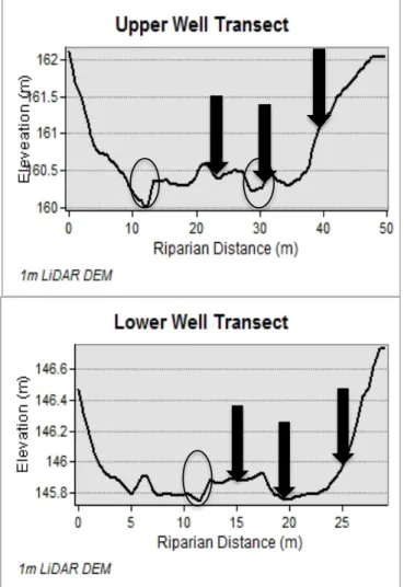
Soil moisture and soil oxygen sensors were installed at the upper and lower riparian transects and in a hillslope hollow (Figure 2.2). Four groundwater wells were installed in approximately 5m increments from the stream to the toeslope at each riparian transect. 1m deep wells 5m from either side of the stream were installed in 2001. The transect was expanded in 2009 with ~2m deep wells that were installed 10m from the 2001 channel in another riparian location and 15 m from the channel at the toeslope.
Soil oxygen sensors were installed at the upper riparian transect in March 2010. These sensors spanned the hillslope-riparian boundary and were placed in a riparian hummock, a riparian hollow, which is the secondary channel, and at the toeslope. Because there was little difference between hummock and toeslope values after 4 months of data collection, we moved the sensor from the hummock to an intermediate position in July of 2010 (Figure 2.3).
In the hillslope hollow adjacent to the upper transect, approximately 40m from the toeslope location, there were two pairs of soil oxygen and water content probes
positioned approximately 20m apart along the trough of the hollow. We collected data from August 2010 to March 2012.
The third datalogger location was in the lower riparian transect. That location had three pairs of soil oxygen and moisture sensors located in riparian hummock, riparian hollow, and toeslope locations. Data were collected at 15-minute intervals from December 2010 to March 2012.
2.3.2 Sensor data
oxygen in air. The diffusion-head sensors were buried vertically with the heads at 6cm depth. Reported sensor accuracy is < 0.002% O2 drift per day. Upon removal in March 2012, oxygen sensors showed no signs of biofouling and atmospheric measurements were within 1% of pre-deployment values. Soil moisture was recorded using Campbell
Scientific CS 616 (Campbell Scientific Inc., Logan, UT) water content reflectometer probes. Probes were installed vertically into the ground and measured the average water content of the top 20cm of soil. Both types of sensors were calibrated before deployment and set to collect soil oxygen and volumetric water content every 15 minutes (hourly at the upper riparian transect). Soil temperature was measured as part of the BES at hourly intervals in upland locations.
2.3.3 Soil nitrogen cycle measurements
Sets of duplicate 10cm long, 5cm wide soil cores were collected via hand auger to measure rates of N cycling in contrasting landscape positions in different seasons. The landscape positions sampled included: riparian hummock, riparian hollow, hillslope hollow, and upland. Cores were sampled in close proximity to the sensors in four different seasons (March, July, and November of 2010 and March, 2011) except at the upland locations where there were no sensors. Upland cores were collected proximal to long-term biogeochemistry plots where soil moisture was recorded monthly and soil temperature was continuously collected at hourly intervals.
Denitrification rates were measured with the N-Free Atmospheric Recirculation Method (NFARM) flow through core measurement system (Burgin et al., 2010, Burgin and Groffman 2012) at the Cary Institute of Ecosystem Studies. The NFARM system replaces air from the sample core with a synthetic atmosphere free of any nitrogen gas, making it easier to measure small changes in N2, a central challenge in measuring denitrification rates (Groffman et al. 2006). Each core was analyzed at 20°C for N2 and N2O fluxes under varying oxygen concentrations (5%, 0%, then10%).
incubation. In situ cores were incubated for approximately four weeks before being returned to the laboratory for analysis. Net nitrification rates were calculated as the increase in nitrate over the course of the incubation period. Net mineralization rates were calculated as the increase in inorganic N (ammonium plus nitrate) over the course of the incubation period. Amounts of ammonium and nitrate were determined by colorimetric analysis with a Lachat Flow Injection Analyzer (Lachat, Loveland, CO). Detection limits for nitrate and ammonium were 0.007 mg/L and 0.002 mg/L N, respectively. The
accuracy or average % recovery for nitrate and ammonium were 100.9 and 97.2%, respectively.
Potential net N mineralization and nitrification and microbial respiration were measured from the accumulation of NH4+ plus NO3- and NO3- alone during 10 day incubations of field moist, mixed soil in the laboratory (Groffman and Crawford 2003). Mineralization and nitrification rates were calculated as described above and respiration was calculated from the accumulation of CO2 over the course of the incubation period. CO2 was
analyzed by gas chromatography.
2.3.4 Water quality analysis
Weekly grab samples were collected at the outlet for the BES LTER site. In addition, longitudinal streamwater samples were collected from a large groundwater seep near the headwaters of the stream at bi-weekly to monthly intervals from April-October 2011. [NO3-] was analyzed on a Dionex Ion Chromatogram (Dionex Sunnyvale, CA).
2.3.5 Geospatial analysis
Terrain Analysis was conducted to determine the areal extent of hillslope hollows and riparian areas. The extent of the riparian zone was delineated based on field collected GPS points and a hillshaded digital elevation model (DEM). Hillslope hollows were delineated for total contributing area above points located on convergent flowpaths located just outside the riparian zone using a LiDAR generated 0.5m DEM. The
extent (perpendicular to the direction of flow) of hollows, the objective here was to more accurately capture the distribution of hummocks and hollows throughout the entire riparian area. Hollows were delineated by selecting a threshold TWI value that matched surveyed classifications using a 0.5m LiDAR DEM with a root mean square error of 0.11 in the vertical dimension (Tenenbaum et al., 2006). Accumulation of contributing
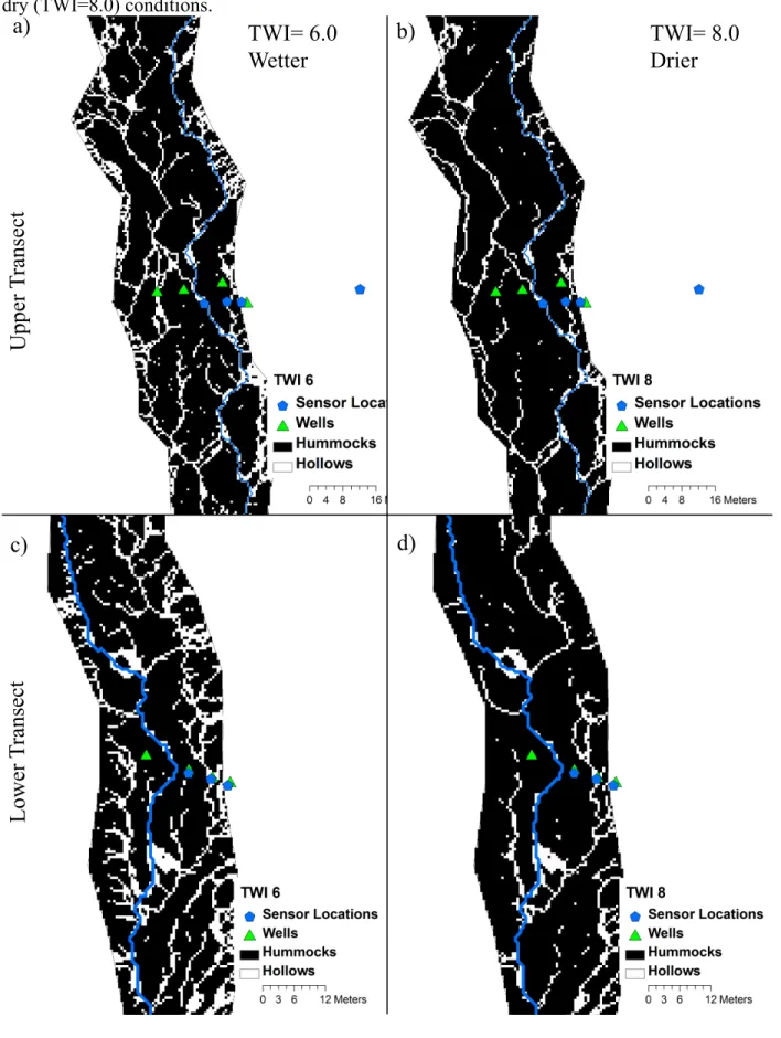
drainage areas were done by preprocessing the DEM for enclosed depressions (pits) using a breaching algorithm (Lindsay and Creed, 2005), and a routing algorithm that enables flow to be partitioned among all downslope patches (D∞) (Tarboton, 1997). Because the hummock and hollow sequences are derived largely from fluvial processes, breaching does not substantially alter the outcome of a binary classification. An auto-level was used in the field to measure elevations at least every 0.5m across valley bottom transects that spanned from toeslope to toeslope. This was then compared with a cross-section from the 0.5m LiDAR with minimal differences found (1 point out of 100 that was more than 10cm off). Based on field verification and surveys, the threshold between hummock and hollow was found to be at a TWI 7.0. Using the mean riparian value (TWI=4.7) as a threshold produced a far larger percentage of riparian hollows than the surveyed value (TWI =7). The difference between TWI thresholds of 6 and 8, span field conditions from wet (just after Hurricane Irene (28-Aug-2011 and Tropical Storm Lee (7-Sep-2011) to dry (July 2011 baseflow) (Figure 2.4). In this range of riparian TWI values, the change in riparian hollow area is not large, ranging from 11 to 18% of total riparian area (Figure 2.5).
2.3.6 Scaling to daily watershed fluxes
probes and oxygen concentrations in the NFARM setup. A Q10 function of 2 (Lloyd and Taylor, 1994) was used to adjust rates for in situ soil temperature. We used upland soil temperature for all landscape positions. Patch flux rates were then extrapolated to the watershed scale based on the total area of each patch type calculated from the terrain analysis.
𝐽= 𝑅∗ 𝜌∗ 𝑣 Equation 2.1
Where J = N2 Flux (g/m2/day), R is the NFARM N2 rate (g/g soil/day) ρ is bulk density (g/ cm3 ) * v is volume per square meter (cm3/m2) (using a 10cm soil horizon depth).
2.3.7 Statistical Analysis
Mean values and standard deviation of soil core parameters were calculated for duplicate cores collected in each of the 4 seasons. A two-way ANOVA was conducted to test for the differences in N2 flux between riparian hollow and all other locations and between riparian locations in the upper transects and the lower transect. Because of variance heterogeneity of N2 flux with oxygen concentration, we used weighted least squares regression. The ANOVA, weighted least squares, and quadratic regression analyses were performed using the software package R (R Development Core Team 2010).
2.4 Results 2.4.1 Soil oxygen
There were marked differences in soil oxygen concentrations among landscape positions and in some locations, across seasons and hydrologic conditions. Soil O2 probes in toeslope and hillslope hummock positions varied from 15 to 21% (Figure 2.6). Because these were so similar and high, we assumed that these sites respond similarly to upland locations. Soil oxygen concentrations in riparian hollows were at 0% for the majority of the year, but increased to a maximum of 11% in the upper transect hollow and 4% at the lower transect hollow during summer dry periods. The most variable sensor was at the upper transect and was located in an intermediate elevation between a hummock and hollow in a secondary channel along the east side of the valley bottom where
by high oxygen concentrations (hillslope hollows and toeslope locations), and one with higher variability (riparian hummocks/intermediate locations) (Figure 2.7). While the aerobic locations were typically at or near atmospheric oxygen concentrations, there were small (<7%) decreases during storms. Hurricane Irene (27-Aug) and especially Tropical Storm Lee (7-Sep) produced decreases in soil oxygen concentration, but never below 10% in aerobic soils.
2.4.2 Seasonal and spatial patterns in nitrogen dynamics
N2 flux rates from upland locations were low at all oxygen concentrations. Rates were highest (p < 0.001) from the riparian hollow cores with intermediate rates found in hillslope hollow cores (Table 2.1, Figure 2.8). N2O flux rates ranged from 0 to 0.029 µg/g/day and were considerably lower than N2 fluxes (0 – 6.0 µg/g/day) (Figure 2.9). Seasonal differences in soil core denitrification were smaller than variability among landscape positions. A two-way ANOVA using landscape position and sample month as main factors showed there was a significant difference in denitrification rates based on landscape position (F = 56.876, P < 0.001) while sample month was not a significant factor (F = 2.573, p < 0.06). A second two-way ANOVA showed that the lower riparian hollow had significantly higher denitrification rates than hummock and upland sites (F = 12.87, P < 0.001) and that differences in sample month were not significant (F = 2.27, P < 0.10). Denitrification rates were consistently higher at 5% O2 than at 0% or 10% O2 (Figure 2.8). The pattern was especially marked in the sites with the highest
denitrification rates (upper hollow, lower hollow, hillslope hollow). We fit quadratic functions between denitrification and O2 for each of these sites (Table 2). While variance of response increased with soil oxygen concentration, this appears to occur as a result of initial soil nitrate concentrations during the March 2010 snowmelt event.
Soil NO3- concentrations were low (< 0.01 g N/kg) for at all sites except during March 2010, which were sampled just after major snowmelt (Table 2.1). In situ net
(Table 2.1). Potential net nitrification ranged from -0.12 to 0.50 g N/kg with no significant differences among sites (Table 2.1).
2.4.3 Annual Potential Mineralization and Nitrification
Estimates of annual in situ net N mineralization and nitrification produced by combining rate and bulk density values in Table 1 and assuming a biologically active season of 270 days ranged from 1.34 to 13.0 g N/m2/y for net N mineralization and from 0.0 to 1.26 g N/m2/y for net nitrification. Estimates of annual potential net N mineralization and nitrification ranged from -3.85 to 8.79 g N/m2/y for net N mineralization and from 0.0 to 17.39 g N/m2/y for potential net nitrification. Potential microbial respiration ranged from 1.01 to 1.67g C/m2/d with no significant differences among sites.
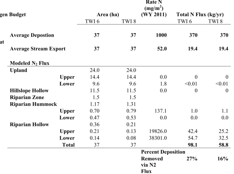
2.4.4 Scaled denitrification estimates
Estimates of daily N2 flux were produced from the quadratic equations relating denitrification to soil O2 (Figure 8) for each landscape position (Equation 1). Riparian hollows were the dominant source of denitrification in the watershed, although there was a small amount of denitrification in the riparian hummocks and at the lower riparian toeslope location during Tropical Storm Lee (Table 2.2). Riparian hollows had significant denitrification activity throughout the year. Upland locations and hillslope hollows did not produce any N2 flux because oxygen concentrations did not reach sufficiently low levels. The highest rates of denitrification (100-175 mg N/m2/day) occurred in riparian hollow cores when they become partially aerated (Figure 2.10).
2.4.5 Watershed nitrogen budget
hillslopes dramatically increases. Similarly, because only the lower upland probe saturated during Tropical Storm Lee, we maintained separate areas for upper (northern and upstream) uplands and lower (southern and downstream) uplands. Because the spatial extent of riparian hollows varies with the selected TWI threshold, we calculated
watershed scale fluxes based on the bracketed values (TWI of 6 under wet conditions and 8 under dry conditions) that we observed through frequent visits to the site under
hydrologic conditions ranging from drought to floods. Groundwater contributions to the overall nitrogen budget are small. Recurrent sampling of a groundwater seep just above the upper transect had low [NO3] of 0.026 mg/L(± 0.005) Cumulative N2 fluxes ranged from 59 to 98 Kg for WY2011 depending on the extent of riparian hollows (TWI of 6 vs. 8). This denitrification is equivalent to 16-27% of the 370 kg N/year that enters the watershed via atmospheric deposition (Table 2.3).
2.5 Discussion
2.5.1 A daily catchment scale budget of denitrification
We were able to combine intact core measurements of denitrification with data from in situ oxygen sensors and terrain analysis to produce estimates of watershed scale