SCENE RECONSTRUCTION BEYOND STRUCTURE-FROM-MOTION AND MULTI-VIEW STEREO
True Price
A dissertation submitted to the faculty at the University of North Carolina at Chapel Hill in partial fulfillment of the requirements for the degree of Doctor of Philosophy in the Department of
Computer Science.
Chapel Hill 2019
Approved by: Jan-Michael Frahm Henry Fuchs Tamara Berg Enrique Dunn
© 2019 True Price
ABSTRACT
True Price: Scene Reconstruction Beyond Structure-from-Motion and Multi-View Stereo (Under the direction of Jan-Michael Frahm)
Image-based 3D reconstruction has become a robust technology for recovering accurate and realistic models of real-world objects and scenes. A common pipeline for 3D reconstruction is to first apply Structure-from-Motion (SfM), which recovers relative poses for the input images and sparse geometry for the scene, and then apply Multi-view Stereo (MVS), which estimates a dense depthmap for each image. While this two-stage process is quite effective in many 3D modeling scenarios, there are limits to what can be reconstructed. This dissertation focuses on three particular scenarios where the SfM+MVS pipeline fails and introduces new approaches to accomplish each reconstruction task.
First, I introduce a novel method to recover dense surface reconstructions of endoscopic video. In this setting, SfM can generally provide sparse surface structure, but the lack of surface texture as well as complex, changing illumination often causes MVS to fail. To overcome these difficulties, I introduce a method that utilizes SfM both to guide surface reflectance estimation and to regularize shading-based depth reconstruction. I also introduce models of reflectance and illumination that improve the final result.
To Luci
Thank you for loving me, and thank you for being there.
In memory of Atul,
ACKNOWLEDGEMENTS
First, I would like to thank my adviser, Jan-Michael Frahm, who has given me so many diverse opportunities to expand my areas of expertise, work with amazing collaborators across many different domains, and challenge myself with supremely interesting research endeavors. This dissertation would not exist without Jan’s patience, commitment, and openness all these years. I would also like to thank the rest of my committee members, Henry Fuchs, Tamara Berg, Enrique Dunn, and Ricardo Mart´ın-Brualla, for their support and feedback. And, I would be remiss if I did not thank Steve Pizer and Julian Rosenman for their guidance, positivity, and unwavering support. I battled so much insecurity and doubt after my first year in graduate school — not that the feeling ever goes away completely, of course! — and I do not think I would have made it without the guidance of Steve, Julian, and Jan-Michael.
I have to extend huge thank you to all of the staff at UNC, as well. From IT staff like Murray Anderegg, Bil Hays, and John Sopko to administrators like Missy Wood, Jody Gregoritsch, and Denise Kenney, there are so many supportive individuals who have gone out of their way to ensure that everything runs smoothly (and, indeed, to keep me in line!). And a special thanks to Jim Mahaney, without whom several research projects would have been dead in the water.
Thanks to all of my co-workers and fellow interns at Organic Motion, Bosch, and Google. I was extremely lucky to get to work with such talented individuals on such exciting projects. These experiences were invaluable to my development as a professional. A special thanks to my mentors: Shaun Kime, Zhixin Yan, and Hugues Hoppe.
TABLE OF CONTENTS
LIST OF TABLES . . . xii
LIST OF FIGURES . . . xiii
LIST OF ABBREVIATIONS . . . xvii
CHAPTER 1: INTRODUCTION . . . 1
1.1 Thesis Statement . . . 4
1.2 Outline of Contributions . . . 4
CHAPTER 2: BACKGROUND AND RELATED WORK . . . 6
2.1 Shape-from-Shading and Shading-based Surface Reconstruction . . . 6
2.2 3D Reconstruction of Endoscopic Imagery. . . 9
2.2.1 Monocular SfM, MVS, and SLAM Techniques . . . 10
2.2.2 Shading-based Approaches and Reflectance Estimation Methods . . . 11
2.2.3 Stereo Endoscopy and Other Semi-Controlled Capture Scenarios . . . 12
2.2.4 Combined Sparse or Dense Reconstruction with Shading Estimation . . . 14
2.2.5 Template-based Reconstruction and Alignment of Pre-operative 3D Scans . . 14
2.2.6 Monocular Depth Estimation via Convolutional Neural Networks . . . 16
2.3 Modeling Transient Objects in Crowd-sourced Imagery . . . 17
2.4 Crowd Simulation in Virtual Representations of Real Environments . . . 19
CHAPTER 3: 3D RECONSTRUCTION OF ENDOSCOPIC VIDEO . . . 21
3.1 Background . . . 24
3.1.1 Reflectance Models . . . 24
3.1.3 Structure-from-Motion . . . 27
3.2 Method . . . 28
3.2.1 Initial PDE . . . 30
3.2.2 Regularization . . . 30
3.2.3 Solving the PDE . . . 32
3.2.3.1 Discretization . . . 32
3.2.3.2 Applying the Lax-Friedrichs Hamiltonian . . . 33
3.2.3.3 Fast Sweeping Scheme and Boundary Conditions . . . 34
3.2.4 Computingσx i,j andσ y i,j for Arbitrary BRDFs . . . 35
3.2.5 Image-weighted Finite Differences . . . 37
3.2.6 Reflectance Model . . . 38
3.2.6.1 BRDF Basis . . . 38
3.2.6.2 Proposed Reflectance Model . . . 39
3.2.6.3 Relation to Other Reflectance Models . . . 40
3.2.7 Iterative Update Scheme . . . 42
3.2.7.1 Warping . . . 43
3.2.7.2 Reflectance Model Estimation . . . 43
3.2.7.3 SfS with Estimated BRDF . . . 44
3.2.7.4 Iteration . . . 44
3.2.8 Accounting for Interreflections in Real Endoscopic Scenarios . . . 46
3.3 Evaluation . . . 48
3.3.1 Comparison of BRDF Fits . . . 48
3.3.2 Ground-truth Geometric Evaluation . . . 52
3.3.3 Results on Patient Data . . . 54
3.4 Discussion . . . 54
4.1 Approach . . . 62
4.1.1 Person Detection and Gravity Estimation . . . 62
4.1.2 Voting-based Scale Estimation . . . 65
4.1.3 Scale Refinement, Height Estimation, and Ground Surface Estimation . . . 68
4.1.4 Ground Surface Reconstruction . . . 72
4.1.5 Visualization . . . 72
4.2 Evaluation . . . 73
4.3 Ablative Analysis . . . 78
4.3.1 Visibility Constraint During Voting . . . 78
4.3.2 Effect of Scale Refinement Terms . . . 79
4.3.3 Effect of Parameters during Refinement . . . 79
4.3.4 Comparing Scale Voting and Scale Refinement . . . 80
4.4 Discussion . . . 80
CHAPTER 5: LIVING 3D RECONSTRUCTIONS . . . 82
5.1 Robust Surface Reconstruction . . . 84
5.1.1 Truncated Signed Distance Function Aggregation . . . 84
5.1.2 Regularizing the Distance Field . . . 87
5.1.3 Optimizing the Distance Field . . . 90
5.1.4 Gravity-aligned Surface Prior . . . 91
5.1.5 Scenario-specific Considerations and Implementation . . . 93
5.2 Triangle Color Estimation and Walkable Area Extraction . . . 94
5.3 Crowd Simulation and Visualization . . . 96
5.4 Results. . . 96
5.5 Discussion . . . 97
CHAPTER 6: CONCLUSION AND FUTURE WORK . . . 107
6.1.1 Extensions to Shading-based Endoscopic Reconstruction . . . 108 6.1.2 Extensions to 3D Reconstruction of Transient Objects and Living
3D Reconstructions . . . 110 APPENDIX A: DERIVATION OF ARTIFICIAL VISCOSITY VALUES IN SFS
LIST OF TABLES
Table 3.1 – Radiance fitting accuracy for MERL materials. For each material, the yellow cell marks the smallestK for which the proposed model
achieved a smaller error than the Phong model. . . 51 Table 3.2 – Accuracy of the proposed SfM+SfS approach for different reflectance
models on simulated and real data across 100 images. Example
render-ings are show in the right column. . . 55 Table 3.3 – Ablation analysis of the proposed method on ground-truth endoscopic
data withK = 2. . . 59 Table 3.4 – Accuracy of the proposed SfM+SfS approach on real endoscopic video
without accounting for surface interreflections. . . 59
Table 4.1 – Quantitative results on the proposed method for scale and placement. “% Error” gives the amount that the method over/under-estimated the
distance of one unit in the reconstruction. npandnc show the number
of placed detected people and photographers, respectively, recovered by
the method. . . 76 Table 4.2 – Ablative analysis on the importance of different parts of the proposed
algorithm. GT: Ground-truth scene scales (reconstruction units per meter). Initial/Final: Estimates from the voting and refinement stages. No Height/Visib.: Height/visibility terms removed from final optimiza-tion. ±10: With all parameters modified by ten percent. Red cells: Results where the estimated length of one unit in the reconstruction was
LIST OF FIGURES
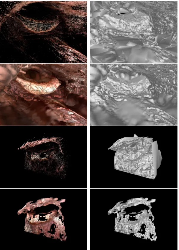
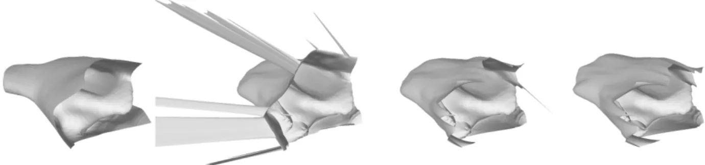
Figure 3.1 – Surface estimates using multi-view stereo reconstruction tend to be noisy and/or incomplete for endoscopic data. Top row: Fused point cloud obtained via MVS (Sch¨onberger et al., 2016) and an untextured surface reconstructed from this point cloud using a method based on the Delaunay tetrahedralization approach of Labatut et al. (2009). Second row: Textured and untextured views of the surface obtained using Poisson surface reconstruction (Kazhdan and Hoppe, 2013) on the MVS point cloud. Bottom two rows: Same results for a different
patient. . . 23 Figure 3.2 – An endoscopogram is constructed via non-rigid registration of multiple
SfMS reconstructions of individual video frames. . . 24 Figure 3.3 – Structure-from-Motion results for endoscopic video. Individual 3D
sur-face points (colored dots) and camera poses (blue) are jointly recovered.
. . . 28 Figure 3.4 – Diagram of the proposed iterative approach for dense surface
recon-struction of a single video frame. . . 29 Figure 3.5 – Compared to the ground-truth surface (left), the boundary conditions
suggested by Kao et al. (2004) can lead to strong artifacts on the edges of the image for endoscopic applications (second from left). A minor change to these conditions can correct for this, although problematic artifacts can still occur (second from right), which can be alleviated by
limiting the maximum surface slope along the image boundary (right). . . 36 Figure 3.6 – The 16 basis functions used in the proposed reflectance model with
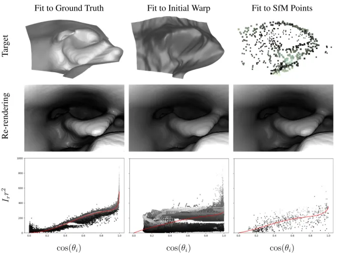
Figure 3.7 – Example fitting results for theK = 5model, using the ground-truth surface (left), warped surface (middle), and sparse SfM points (right) on a synthetic image. The top row shows the initial surfaces and points use for the fitting; these target values are scattered in the graphs in the bottom row, with each value colored by its observed intensity for visualization. The red curves in the bottom row plot the reflectance function η(θi;Θ)whose parameters Θhave been robustly fit to the
plotted points. The middle row shows a re-rendering of the ground-truth surface using these fit functions. Fitting to the SfM points alone is more reliable than fitting to the entire warped surface, which may contain errors in depth as well as incosθi. In this example, the
near-specular effects of the material are better captured by the fit using the
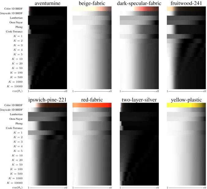
SfM points. . . 45 Figure 3.8 – Estimated 1D radiance functions for different materials from the MERL
database (Matusik et al., 2003). The top row of each image shows the color radiance,cos(θi)BRDFλ(θi), and the second row shows the
luminance equivalent. Subsequent rows show least-square fits to the
luminance function for different BRDF models. . . 49 Figure 3.9 – Visual comparison of surfaces generated by the proposed approach for
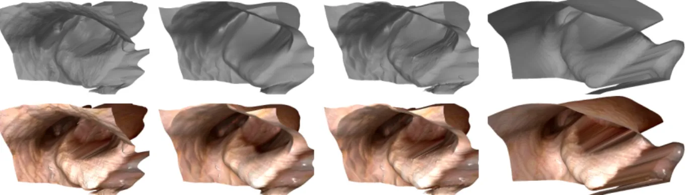
an image from a ground-truth dataset. Top/bottom rows: Visualization of the surface without/with texture from the original image. Columns from left to right: (1) using a Lambertian BRDF, (2) using the proposed BRDF (K = 2) without image-weighted derivatives, (3) using the proposed BRDF (K = 2) with image-weighted derivatives, and (4) the ground-truth surface. Note the oversmoothing along occlusion boundaries in column (2) versus column (3) and the flattened curve of
the epiglottis in column (1). . . 53 Figure 3.10 – Example results for three images from a live endoscopic video. Left:
Original image. Right: Surface estimated from the image using the
proposed algorithm. . . 56 Figure 3.11 – Example results for three images from a live endoscopic video. Left:
Original image. Right: Surface estimated from the image using the
proposed algorithm. . . 57 Figure 3.12 – Example results for three images from a live endoscopic video. Left:
Original image. Right: Surface estimated from the image using the
proposed algorithm. . . 58
Figure 4.2 – To accurately localize 2D ground points for detected people, a planar torso model in 3D (left) is first fit to detected 2D neck, shoulder, and
hip joints (middle-left). Right: Coordinate axes for the planar model. . . 65
Figure 4.3 – Scale scoring curve for a model of the Pantheon. The peak is chosen as the initial scale estimate. . . 68
Figure 4.4 – Overhead views (left) and sample renderings with ground and person avatars (middle) for the proposed method. Examples of real photos are shown on the right. The green dots in the overhead views show person placements, with cameras as red dots and detected people as green dots. Black dots show static structure. From top: Dubrovnik, Croatia; the Pantheon; San Marco Plaza, Venice; and the area around the Colosseum and Roman Forum in Rome. . . 74
Figure 4.5 – Overhead visualizations of person placements (left) versus aerial views from Google Earth (right). From top to bottom: Buckingham Palace, the Palace of Westminster, the Sacr´e Cœur in Paris, Trafalgar Square, and Trevi Fountain. . . 77
Figure 4.6 – Result of the scale voting scheme with (blue) and without (orange) the visibility constraint. The ground-truth scale is near 0.01 reconstruction units per meter. . . 78
Figure 4.7 – Ratio of the estimated neck distances||Ni||to the visibility threshold vi(s) for the ground-truth scale (GT), and for larger/smaller scales. Values are sorted and clipped to[0.5,1.5]. . . 79
Figure 5.1 – Left: A scene mesh generated by point cloud fusion from MVS depthmaps and Delaunay tetrahedralization with visibility optimization (Sch¨onberger et al., 2016). Middle: Mesh for the same approach, with 3D ground points of detected people added to the point cloud. Right: Scene mesh generated by the proposed method. . . 83
Figure 5.2 – Initial labeled ground triangles (white) and additional triangles added after the proposed region-growing approach (red). . . 96
Figure 5.3 – Qualitative, ablative comparison of scene reconstruction results for the Tower of London under the proposed implementation at a voxel resolution of 1m. . . 98
Figure 5.4 – Reconstruction of Buckingham Palace. . . 99
Figure 5.5 – Reconstruction of the Castel Sant’Angelo in Rome. . . 100
Figure 5.7 – Reconstruction of the Old Town Square in Prague. . . 102
Figure 5.8 – Reconstruction of the Piazza San Marco in Venice. . . 103
Figure 5.9 – Reconstruction of the Sacr´e Cœur Basilica in Paris. . . 104
Figure 5.10 – Reconstruction of the Tower of London. . . 105
LIST OF ABBREVIATIONS
BRDF Bidirectional Reflectance Distribution Function
GT Ground Truth
LF Lax-Friedrichs
MVS Multi-View Stereo
PDE Partial Differential Equation SfM Structure-from-Motion
SfMS Shape-from-Motion-and-Shading
SfS Shape-from-Shading
TSDF Truncated Signed Distance Function
CHAPTER 1: INTRODUCTION
The observable world is made up of tangible materials with well-defined physical properties and spatial relationships. For example, we could identify a building as being covered in brick and having a specific length, width, and height in meters. The action ofobservingsuch an object, however, is an indirect process. For instance, an observer such as the human eye or a pinhole camera does not “see” a brick building in a three-dimensional sense, but rather collects information about the intensity and distribution of visible light rays irradiating and then reflecting from the building’s surface towards the observer. This is the driving problem of 3D reconstruction in computer vision: Given that an image only provides us with a 2D slice of visible light rays, how can we recover the underlying 3D surfaces that effected the image?
images; these approaches attempt to learn shape constraints automatically from 2D appearance by training on a large number of images, given ground-truth depth maps or corresponding stereo image views (Eigen et al., 2014; Garg et al., 2016; Godard et al., 2017; Zhou et al., 2017; Li and Snavely, 2018).
Multi-image reconstruction methods seek to recover the underlying surfaces of an environment using images taken from multiple vantage points within the space. Approaches in this vein typically consist of a “sparse, then dense” pipeline, although many variations exist for different reconstruction scenarios. The most general “sparse” reconstruction approach is known as Structure-from-Motion (SfM) (Pollefeys et al., 2004; Snavely et al., 2006, 2008; Frahm et al., 2010; Agarwal et al., 2011; Crandall et al., 2011; Wu, 2013; Wilson and Snavely, 2014; Heinly et al., 2015; Sch¨onberger and Frahm, 2016).1 Given a set of images, SfM aims to jointly recover camera intrinsics, relative
image poses, and the 3D position for corresponding points in the individual images. The method is “sparse” because, rather than obtaining a surface with fixed fiducial sampling in the 3D world or 2D pixel space, points on the 3D structure are determined only for locations in the images with highly distinguishable 2D appearance. SfM is typically used as a preprocessing step for “dense” multi-image reconstruction techniques such as multi-view stereo (MVS) (Furukawa and Ponce, 2010; Furukawa et al., 2010, 2015; Sch¨onberger et al., 2016). Like SfS, MVS recovers a depth map for each individual image. However, instead of using strong assumptions on illumination and surface conditions, MVS utilizes the fact that an image point will have similar appearance in nearby viewpoints if it is lifted into 3D and then reprojected into the other view. The correct underlying surface for an image, therefore, is determined by maximizing appearance similarity after reprojection. After multiple depth maps are obtained via MVS, a final model of the scene can be recovered by fusing and meshing these individual surfaces within the global space of the reconstruction (Curless and Levoy, 1996; Labatut et al., 2009; Jancosek and Pajdla, 2011; Sch¨onberger et al., 2016).
1
All three methods – SfS, SfM, and MVS – and their variants have limitations that impair or prohibit reconstruction in certain scenarios. For example, the equations governing SfS may be difficult to model for sufficiently complex surfaces and lighting conditions, and in any case, the underlying material reflectance properties must be well defined. SfM and MVS, on the other hand, strictly assume that the underlying 3D surfaces are stationary in all images; they are unable to handle dynamic objects. Although non-rigid SfM (NRSfM) with monocular (Bregler et al., 2000; Xiao et al., 2004; Akhter et al., 2009; Garg et al., 2013; Russell et al., 2014) and multi-view (Zheng et al., 2015; Ji et al., 2016; Innmann et al., 2019) formulations2 have proven successful in certain reconstruction scenarios, rigid and non-rigid methods alike are strongly limited by the distinguishability of the underlying surface appearance and by the conditions in which the images were taken. For instance, homogeneous regions in images lack distinguishing texture and thus are difficult to reliably identify between images, which reduces reconstructability. Even for potentially well-textured surfaces, appearance can change due to the time of day or weather, and surfaces like the ground may only be captured from unfavorable angles in the majority of images; these imaging conditions frequently occur in Internet photo-collections (Kuhn et al., 2017). For dynamic object reconstruction, temporal sampling also comes into play, as existing approaches like NRSfM require the temporal order of images to be known and well-sampled. This works for reconstructing objects in video sequences, but for objects that are only imaged once, such as pedestrians in a temporally sparse photo-collection, it is necessary to develop methods that do not assume temporal contiguity. Finally, due to the properties of perspective projection, all reconstruction approaches are only accurate up to scale without additional prior knowledge on the expected size of imaged objects.
In this dissertation, I address 3D reconstruction scenarios with imaging conditions that are unfavorable due to an inability to leverage temporal consistency and/or due to insufficient surface texture for discriminative dense multi-view correspondence identification. Tackling these challeng-ing reconstruction problems requires significant and novel adaptions to the traditional approaches listed above. Details of the individual research thrusts that support this thesis are provided below.
2
1.1 Thesis Statement
In 3D reconstruction scenarios where the typical conditions of structure-from-motion and multi-view stereo are violated for specific objects or surfaces, more complete 3D representations can be obtained through additional processing that combines multi-view reasoning and scenario-specific constraints.
1.2 Outline of Contributions
The body of work in this dissertation covers multiple scenarios in 3D computer vision that traditional robust modeling techniques cannot handle:
3D Reconstruction of Endoscopic Video: I introduce a new approach for reconstructing dynamic,
poorly textured surfaces inside the human body. To overcome the difficulties in this 3D modeling scenario, my method employs a combination of sparse 3D modeling, shading constraints, and integrated regression of surface reflectance parameters. This work, detailed in Chapter 3, has been partly described in several publications (Zhao et al., 2015, 2016; Wang et al., 2017). Chapter 3 also contains expanded research regarding the approach, detailing new aspects of the formulation and optimization that lead to improved accuracy.
3D Reconstruction of Transient Objects: I propose a novel approach for augmenting 3D
CHAPTER 2: BACKGROUND AND RELATED WORK
The three following chapters of this dissertation generally fall into two major categories: performing 3D reconstruction on endoscopic video data using shading and structure, and modeling humans in 3D environments reconstructed from Internet photo-collections. In the following sections, I provide a broad general background of endoscopic reconstruction and outline approaches related to 3D reconstruction and human modeling in large-scale datasets.
2.1 Shape-from-Shading and Shading-based Surface Reconstruction
While older methods exist for SfS under general illumination and reflectance, for example the work of Zheng and Chellappa (1991) and Tsai and Shah (1994), these methods have long been known to perform poorly even given synthetic data, partially due to simplified assumptions of reflectance, lighting, and camera projection (Zhang et al., 1999). Traditional PDE formulations of SfS assume a Lambertian reflectance model for the scene (Visentini-Scarzanella et al., 2012), which may be a poor assumption for real-world data (Zhang et al., 1999; Ahmed and Farag, 2006). Some work has investigated non-Lambertian models for the SfS PDE formulation. Ahmed and Farag (2006) introduce a SfS method for the Oren-Nayar reflectance model, which describes reflectance for rough diffuse surfaces; the authors later demonstrated an approach for the Ward reflectance model (Ahmed and Farag, 2007). Vogel et al. (2009) present a method for SfS on Phong-type surfaces, which is itself an extension of the Lambertian model with added ambient and specular terms. Qu´eau et al. (2017) formulated a SfS PDE for scenes exhibiting known natural illumination and albedo. For endoscopic applications, I propose a reflectance model that subsumes the Lambertian and Phong models and, in general, is suitable for surfaces with arbitrary reflectance properties. To avoid a need to know the reflectance modela priori, I also introduce an approach for using Structure-from-Motion (SfM) to bootstrap reflectance model estimation and guide the SfS solution.
Smith (2011) utilize silhouette constraints to avoid the requirement of an explicit reflectance map. Both of these methods utilize the fact that diffuse surfaces act as low-order filters of the environment illumination, and thus the illumination can be approximated using low-order spherical harmonics.
Deep learning methods have much promise in robustly modeling the complex shading behaviors found in real-world applications of the inverse graphics problem. In particular, Li et al. (2018) recently introduced a convolutional neural network approach for jointly estimating albedo, specular roughness, surface normal, and depth for an object captured in a single flash-illuminated image. The approach also estimates environment illumination for the image and introduces an internal network architecture to recover images formed from multiple bounces of light off of the surface; an analytical rendering layer is used to produce the direct illumination image based on the regressed surface parameters. The network applies a multi-stage refinement of estimated parameters to achieve state-of-the-art recovery of shape and reflectance parameters from a single image.
2.2 3D Reconstruction of Endoscopic Imagery
In Chapter 3 of this thesis, I motivate endoscopic surface reconstruction for 3D review during treatment planning. That is, given an endoscopic video, use an offline reconstruction process to build a textured surface model of the target area that a physician can for enhanced visualization, video review, or procedure post-analysis. In addition to treatment planning, the literature is rife with methods that target goals for augmented reality and real-time 3D applications during surgery. I address the general themes and research areas in this section.
To provide some historical context, methods for achieving 3D reconstruction of endoscopic imagery have existed for at least three decades, dating back at least to the early work of Badiqu´e et al. (1988) that investigated correlation-based matching and 3D visualization for stereoscopic endoscopy. The work of Oda et al. (1994, 1995a) was perhaps the first to outline a full approach for 3D reconstruction from monocular endoscopic video. Similar to the standard pipeline of today’s reconstruction methods, this method introduced a SfM-type sparse reconstruction approach with inter-frame feature tracking and proposed a method for patch-based multi-view depthmap estimation, with later extensions to estimate the scale of the reconstruction based on light intensity (Oda et al., 1995b). Perhaps the earliest applications of SfS for endoscopy were introduced by Deguchi (1996), Okatani and Deguchi (1997), and Yeung et al. (1999), who used a method for estimating equal-depth contours to recover shape from a single endoscopic image assuming a known — but material-agnostic — 1D Bidirectional Reflectance Distribution Function (BRDF). The first two works actually utilize multi-view information as part of the method, initializing the estimation using a sparse, multi-frame surface estimation algorithm (Deguchi et al., 1994). The third work is the first that I know of to empirically measure a BRDF for use in endoscopic SfS.
Still other methods —e.g., Shape-from-Template algorithms — have combined these approaches with pre-operative CT scans that serve as a shape prior for reconstruction or as a target space for reconstruction alignment. Finally, a number of alternative capture strategies such as range imaging and depth-from-focus have been proposed.
2.2.1 Monocular SfM, MVS, and SLAM Techniques
The vast majority of endoscopic procedures are carried out using monocular (single-view) endoscopes, and thus many methods have established monocular approaches to 3D reconstruction that seamlessly integrate with existing treatment planning and surgical workflows (Maier-Hein et al., 2013). Burschka et al. (2005) proposed a SLAM approach for sinus surgery that obtained a sparse surface reconstruction entirely from monocular endoscopic video. Reconstruction scale was obtained via rigid alignment to a CT scan. Other sparse SLAM approaches for monocular endoscopy include the work of Grasa et al. (2011, 2013), which leveraged extended Kalman filters to improve reconstruction accuracy for handheld endoscopic video capture; the work of Marcinczak and Grigat (2014), which adopted a photometric, volumetric approach (Newcombe et al., 2011) that accounts for surface specularities in its photometric cost; and the work of Chen et al. (2018), which applied intraoperative meshing to the reconstructed point cloud with a goal of real-time 3D visualization. Marmol et al. (2018) introduced a keypoint-based SLAM approach for anthroscopy in minimally invasive surgery scenarios; this approach was later extended to perform dense PatchMatch-based MVS (Bleyer et al., 2011) on SLAM keyframes to form a dense global reconstruction (Marmol et al., 2019). Mahmoud et al. (2019) also recently introduced a monocular SLAM system with dense multi-view depth estimation for selected keyframes.
scan was then aligned to this sparse result to compute a 2D/3D registration. Several approaches have proposed to obtain a reconstruction solely from SfM and then perform single-frame or global surface reconstruction from the resulting point cloud Thormahlen et al. (2002); Sun et al. (2013); Lurie et al. (2017). However, these methods are strongly dependent on the completeness and accuracy of the SfM result. Considering newer technologies for external 6-DoF tracking of the endoscopic device, Garbey et al. (2018) assessed sparse surface reconstruction for laparoscopic scenarios where the absolute camera pose is known.
2.2.2 Shading-based Approaches and Reflectance Estimation Methods
As mentioned above, single-image shape-from-shading approaches have long been applied to endoscopic imagery. For example, Tankus et al. (2005) demonstrated some of the first SfS results on medical images following the introduction of the perspective PDE formulation for SfS. Visentini-Scarzanella et al. (2012) applied Lambertian SfS on endoscopic images with a non-co-located light source and proposed an approach for scale recovery by triangulating surface specularities. Wu et al. (2010) introduced a multi-view surface reconstruction approach leveraging Lambertian shading and known camera motion in the context of bone reconstruction. Their approach first performs single-view SfS on individual images, aligns these individual surfaces, and progressively introduces multi-view surface consistency constraints to refine and fix the estimated SfS depthmaps. I further discuss multi-view extensions of shading-based surface estimation in a later subsection.
render the CT surface from novel views. Nunes et al. (2017) similarly estimate the BRDF of a liver using a video-aligned CT scan after manual non-rigid 2D/3D alignment.
Finally, one quite different single-frame depth estimation method that is worth mentioning is the approach of Hong et al. (2009, 2014), which is specifically tailored for the 3D reconstruction of colonoscopic images. This approach explicitly models the “tube with folds” anatomy the colon and uses reasoning about light intensity to compute slant directions. However, the approach does not generalize to other anatomical structures.
2.2.3 Stereo Endoscopy and Other Semi-Controlled Capture Scenarios
Many methods have focused on reconstruction using binocular stereo endoscopes, which recover per-frame depth using photometric matching between a synchronized pair of cameras; this synchronized matching leads to a much more controlled reconstruction problem Mountney et al. (2010). Stereo approaches have frequently been combined with SfM- or SLAM-type approaches for complete surface reconstruction, and 3D stereoscopic endoscopy has recently shown potential for improving treatment outcomes versus traditional monocular endoscopy (Albrecht et al., 2016; Egi et al., 2016; Best, 2019; Bickerton et al., 2019). Considering multi-view reconstruction approaches, one early SfM-type approach from Kitoh et al. (1998) proposed to use a stereo endoscope for accurate scale estimation. Later efforts include the work of Lau et al. (2004) that proposed a method using stereo endoscope observations to monitor cardiac deformations caused by heatbeats and respiration. Mountney et al. (2006) introduced the first (sparse) stereoendoscopic SLAM approach for minimally invasive surgery; further work introduced coarse surface stitching from the sparse reconstruction (Mountney and Yang, 2009) and an altered SLAM approach to compensate for the periodic motion caused by respiration (Mountney and Yang, 2010). A number of other stereo SLAM approaches have been introduced since this initial work, targeting areas such as robust tracking in rigid Chang et al. (2014) and deforming (Lin et al., 2013) environments.
complete surface reconstruction, which can be used in a stereoscopic SLAM system (Reichard et al., 2016). Motivated towards real-time AR surgery applications, Chen et al. (2017) also proposed a stereo SLAM approach with depthmap fusion. Recently, Song et al. (2018) introduced a real-time stereo SLAM approach that is able to handle deforming surfaces and demonstrated aligned depthmaps for a number of endoscopic video sequences. Apart for multi-view reconstruction approaches, a number of works have explored improving, post-processing, and evaluating stereo depthmap estimation algorithms for endoscope-specific applications, particularly with a goal of overcoming the inherent difficulties of stereo reconstruction for low-texture surfaces (R¨ohl et al., 2011; Stoyanov et al., 2010; Chang et al., 2013; Parchami and Mariottini, 2014; Totz et al., 2014; Wang et al., 2018; Zampokas et al., 2018).
Lin et al. (2016) and Bernhardt et al. (2017) for further discussion on active and stereo endoscopic reconstruction methods.
2.2.4 Combined Sparse or Dense Reconstruction with Shading Estimation
A number of works have explored the combination of shading models with multi-view recon-struction methods. Kaufman and Wang (2008) proposed to use SfM to obtain camera motion and Lambertian SfS to obtain per-frame depth; however, the authors reported that the success of depthmap fusion in their method was hindered by inaccuracies in the SfS estimates. Tokgozoglu et al. (2012) used multi-view stereo to derive a low-frequency model of the upper airway, then applied Lambertian SfS on albedo-normalized images to endow the existing surface with higher-resolution shape. Turan et al. (2017) achieved non-rigid SLAM by using SfS to estimate per-frame depth combined with inter-frame point tracking and depthmap-to-fused-model surface registration. These authors later introduced a camera tracking method that performs per-frame depth estimation using Lambertian SfS and then feeds the resulting RGB-D image into a recurrent neural network to regress 6-DoF camera motion (Turan et al., 2018). Several other works have explored shading-based alignment of pre-operative 3D scans to endoscopic imagery. I discuss these approaches in the following subsection.
2.2.5 Template-based Reconstruction and Alignment of Pre-operative 3D Scans
two-stage process of texture-based alignment followed by shading-based refinement; the CT texture is obtained from the previous video frame (assuming an initial alignment), and shading is refined by rendering the CT surface and minimizing the overall squared intensity difference. Later work expanded this approach to include image-based tracking with alignment to the CT scan (Mori et al., 2002). Helferty and Higgins (2002) used a preoperative CT scan as a geometry proxy for camera tracking in bronchoscopy under rigid surface assumptions. Assuming an initial alignment of the CT to the video is available, this method estimates the relative camera motion between frames via an optical flow (i.e., intensity matching) formulation that utilizes the 2D motion constraints induced by project of the CT surface. The method was later extended to use an alignment procedure assuming Lambertian shading (Helferty et al., 2007) and was used to perform image-based texturing of the CT mesh (Rai and Higgins, 2006).
Rigid registration was also used by Vagvolgyi et al. (2008) to align single-frame stereo endoscope depth estimates to a CT mesh. Mirota et al. (2009) proposed to use a trimmed iterative closest point approach to rigidly align a preoperative CT scan to a 3D point cloud created using an SfM-type type approach for endoscopic video (Wang et al., 2008). Bernhardt et al. (2015) performed rigid 3-DoF camera-to-CT-surface alignment assuming local Lambertian shading and albedo in the image; this approach is in contrast to other shading-based alignment approaches that assume reflectance properties hold globally across the image. Billings and Taylor (2015) introduced an iterative alignment procedure to rigidly align two oriented point clouds. Sinha et al. (2018) extended this work to deformably register a surface representation of the nasal cavity and sinuses to a meshed SfM point cloud recovered from endoscopic video; unlike the methods mentioned above, this approach uses a shape space learned from extracted CT surfaces and does not require a patient-specific CT scan.
subsequently adjusted to match. Others have proposed methods for deformable registration of a CT preoperative scan to sparse stereo-based reconstructions (Haouchine et al., 2014), partial surfaces Song et al. (2016), and time-of-flight endoscopic imagery (dos Santos et al., 2014).
2.2.6 Monocular Depth Estimation via Convolutional Neural Networks
The recent explosion of convolutional neural networks for image processing has encouraged interesting alternatives to classical approaches for 3D reconstruction, including for endoscopies. Reiter et al. (2016) proposed an interesting approach to train a patienti-specific neural network that regresses per-pixel depth and normal information solely as a function of position in the image and pixel color. This technique bypasses explicit surface reflectance and illumination modeling, which avoids the common pitfalls of pure shading-based modeling. However, the approach requires careful 3D alignment of the endoscopic video frames to a preoperative CT scan for each specific patient in order to train against a ground-truth surface, and it is unclear how well the method would generalize between patients or to environments where direct CT registration is impossible. Mahmoodet al. (Mahmood and Durr, 2018; Mahmood et al., 2018) perform direct monocular depth estimation using a convolutional neural network with refinement via a conditional random field. A similar approach was taken by Visentini-Scarzanella et al. (2017), who learn to regress depth from virtual CT images and, to apply this network to real imagery, train a separate network to re-render real images to look like virtual CT images. Training this second network again requires 2D/3D registration of a CT surface to its corresponding real endoscopic video sequence.
depth estimation. Having such a fallback is quite useful when processing endoscopic video. This is because an endoscopic video may only contain short snippets of “good” imagery due to, for example, constant patient motion. Since some parts of the anatomy may therefore only be glimpsed very briefly, it may be necessary to drop temporal constraints for these frames in order to reconstruct them.
2.3 Modeling Transient Objects in Crowd-sourced Imagery
There has been a strong interest in automatically obtaining 3D reconstructions from crowd-sourced images. The seminal work of Snavelyet al. (Snavely et al., 2006, 2008) demonstrated the feasibility of reconstruction from Internet photos, and later systems robustified the reconstruction methods and tackled increasingly larger scenes and photo-collections. Today, state-of-the-art systems are able to provide highly detailed 3D models of thousands of sites around the world from one-hundred million user-uploaded images (Heinly et al., 2015; Sch¨onberger et al., 2016). However, the resulting models are only reconstructed up to an unknown scale factor and only represent the static parts of the scenes. Transient objects such as humans are inherently missing in such reconstructions.
explored increasing robustness by additionally incorporating vanishing points from the static scene. For general crowd modeling in multi-view synchronized systems (Wang, 2013), a large number of methods (e.g. (Ge and Collins, 2010; Fleuret et al., 2008; Otsuka and Mukawa, 2004; Focken and Stiefelhagen, 2002; Black et al., 2002)) exist to triangulate and track people in the camera space, potentially without explicit correspondences (Liu et al., 2013) or a knowledge of the system calibration (Guan et al., 2016). All of these works, however, either assume that the temporal domain is densely sampled or only perform a calibration task for a single camera. Multi-view reconstructions from internet photo-collections, in contrast, consist of potentially tens of thousands of unique, temporally disjoint images.
Finally, Bulbul and Dahyot (Bulbul and Dahyot, 2016) introduced a method for obtaining representations of transient objects in map representations such as OpenStreetMap (OSM). In contrast to large-scale 3D reconstructions from unordered Internet photo-collections, OSM provides both a to-scale, geo-localized environment model and a coarse ground surface representation. The authors used social media photos with geo-localization metadata to place human avatars into the map. To obtain the camera position of a social media image, they registered the image to nearby Google StreetView (GSV) images based on its known geo-location. People in the images were placed onto the map’s ground surface at a distance from the camera estimated by the size of their face in the image. For visualization, realistic poses and configurations for virtual people were introduced, and the authors also simulated crowd flow for the agents to move from different photograph locations within the OSM environment. While this approach places humans into 3D environments, the method relies on a large amount of data (scene scale, OSM models, GPS data, social media timestamps, and GSV imagery) that is typically unavailable for general large-scale 3D reconstructions.
2.4 Crowd Simulation in Virtual Representations of Real Environments
CHAPTER 3: 3D RECONSTRUCTION OF ENDOSCOPIC VIDEO
Endoscopy is a common medical procedure wherein a camera with a light attached is inserted into the body, allowing physicians to gain a direct view of the internal surfaces of a patient without resorting to strongly invasive methods. Endoscopic medical vision applications constitute a steadily growing field of 3D computer vision research with much potential to improve patient outcomes without significant alterations to existing physician workflows. For example, a doctor performing laparoscopic surgery uses video to as a navigational aid during the procedure. By performing online 3D reconstruction on this video as it is captured, medical vision technologies can augment the surgeon’s spatial reasoning during the procedure.
can exceed 40 minutes in length, which prohibits review to determine whether growths were missed or potentially unobserved.
Constructing an endoscopogram, however, is a challenging task for several reasons, especially in the case of nasopharyngoscopy. For one, the inside surfaces of the throat are stationary for only very short time windows due to the patient breathing and swallowing. This makes traditional SfM techniques difficult to leverage, since the relative camera motion is quite slight relative to surface; from experience, sparse point triangulation is generally possible but quite prone to noise. Compounding this, the throat surfaces are quite homogeneous in appearance, which limits the amount of feature points that can be reliably matched between video frames; this is unfavorable for NRSfM approaches, which typically rely onad hoc point clusterings to build a dynamic motion model. The homogeneous textures and poor triangulation angles also make MVS depth estimates quite noisy, resulting in degraded surface estimates (Fig. 3.1).
Given these difficulties for multi-image reconstruction methods, single-image methods like SfS seem to be a reliable alternative, since they are agnostic to texture homogeneity, camera motion, and surface dynamics. Unfortunately, the near-surface lighting conditions in nasopharyngoscopy make it impossible to derive a global model of illumination/material reflectance that can be applied for all video frames. A successful SfS approach must be able to refine illumination properties on a frame-by-frame basis.
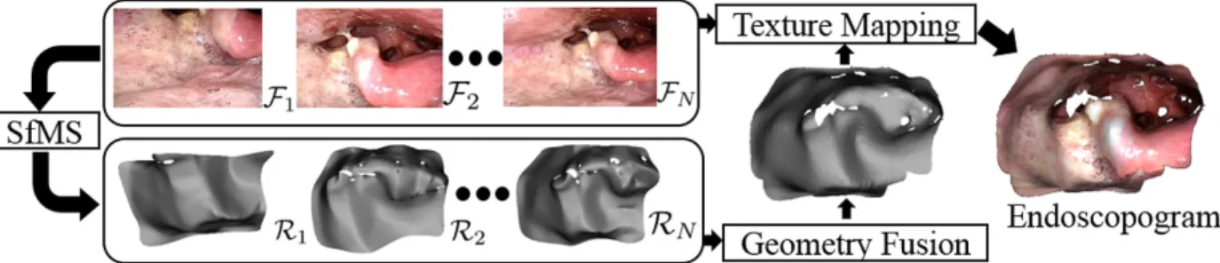
Figure 3.2: An endoscopogram is constructed via non-rigid registration of multiple SfMS recon-structions of individual video frames.
between the previous SfS surface and the shading constraints that arise under the newly estimated illumination/reflectance model. I also propose a new, generalized reflectance model that better accounts for the illumination conditions present in endoscopy, compared to the Lambertian model typically adopted for SfS. Moreover, I propose a simple approach for modeling light interreflections within the endoscopic space that are not accounted for in traditional SfS approaches, and I show that this can substantially improve the accuracy of the depth estimated by SfMS.
Fig. 3.2 outlines the overall process of constructing the final endoscopogram. Once depthmaps have been computed using SfMS for a set of endoscopic video frames, a final endoscopogram can be formed via non-rigid registration of the individual surfaces. This more complete surface can then itself be non-rigidly aligned to the CT surface for visualization within the original treatment planning space. Details of these fusion and registration procedures are described in Zhao et al. (2015), Zhao et al. (2016), and Zhao (2017).
3.1 Background
3.1.1 Reflectance Models
The amount of light reflecting off a surface can be modeled by a wavelength-dependent Bidirec-tional Reflectance Distribution Function (BRDF) that describes the ratio of the radiance of light reaching the observerIλr to the irradiance of the light hitting the surfaceEλr(Cook and Torrance,
given as a function of four variables: the angles(θi, φi)between the incident light beam and the
normal, and the reflected light angles(θr, φr)with the normal; that is,
BRDFλ(θi, φi, θr, φr) =
Iλr
Eλi
, (3.1)
whereλrepresents light wavelength. In the following, the wavelength dependence of the BRDF is implicitly assumed.
The irradiance for an incoming beam of light is itself a function ofθi and the distancerto the
light source:
Ei =Ii
A
r2 cosθi, (3.2)
whereIi is the light source intensity andArelates to the projected area of the light source.
For the case of endoscopy, two simplifying assumptions about the BRDF can be made that help the overall modeling of the problem. The first assumption is that the BRDF exhibits surface isotropy, which constrains it to only depend on the relative azimuth,∆φ=|φi−φr|, rather than the
angles, themselves (Koenderink et al., 1996). While this sacrifices some generality, it provides a good approximation for surfaces with low anisotropy. Second, it is assumed that the light source is approximately located at the camera center relative to the scene, which is a reasonable model for many endoscopic devices. In this case, the incident and reflected light angles are the same,i.e. (θi, φi) = (θr, φr). Under these assumptions, the observed radiance simplifies to
Ir(r, θi) =Ii
A
r2 cos(θi)BRDF(θi). (3.3)
3.1.2 Surface Model for Shape-from-Shading
to 3D locations on a surface viewed by the camera. Under perspective projection,
f(x, y) =z(x, y)
x y 1 , (3.4)
wherez(x, y) >0is a mapping from the image plane to depth along the camera’s viewing axis. The distancerfrom the surface to the camera center is
r(x, y) =kf(x, y)k=z(x, y)px2+y2+ 1, (3.5)
and the normal to the surface is defined by the cross product between thexandyderivatives off:
n(x, y) =fx×fy =z
−zx
−zy
xzx+yzy +z
. (3.6)
The lighting conditions of the endoscope allow us to assume that the scene is illuminated by a single light source located at the optical center of the camera. In this case, the light direction vector for a point in the image is the unit vectorˆl(x, y) = √ 1
x2+y2+1(x, y,1). The cosine of the
angleθi(x, y)between the normal and light direction vectors is then equal to their dot product:
cosθi =nˆ·ˆl=
z
q
(x2+y2+ 1) z2
x+z2y + (xzx+yzy+z)2
,
(3.7)
Prados and Faugeras (2005) note that Eq. (3.7) can be simplified using the change of variables v(x, y) = lnz(x, y):
ˆ
n·ˆl= q 1
(x2+y2+ 1) v2
x+v2y+ (xvx+yvy+ 1)2
.
(3.8)
This transformation allows us to separate terms involvingvfrom those involving its derivatives in our shading model, which is important for PDE formulations of the SfS model.
3.1.3 Structure-from-Motion
As mentioned previously, Structure-from-Motion (SfM) (Hartley and Zisserman, 2003; Pollefeys et al., 2004; Sch¨onberger and Frahm, 2016) is the simultaneous estimation of camera motion and 3D scene structure from multiple images taken at different viewpoints. Typical SfM methods produce a sparse scene representation by first detecting and matching local features in a series of input images, which are the individual frames of the endoscope video in our application. Then, starting from an initial two-view reconstruction, these methods incrementally estimate both camera poses and scene structure. The scene structure is parameterized by a set of 3D points projecting to corresponding 2D image features.
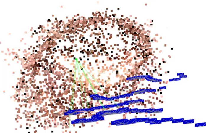
In the case of endoscopy, the motivation for using SfM is that it provides a (sparse) prior on depth, which supplies adequate constraints for surface geometry and reflectance estimation. Because SfM uses rich feature descriptors to identify image correspondences, compared to the weaker photo-consistency metrics of multi-view approaches, experience shows that SfM produces substantially more reliable, albeit sparse and typically noisy, geometry for endoscopic datasets. Fig. 3.3 shows an example SfM reconstruction of endoscopic data using several segments from the overall video.
Figure 3.3: Structure-from-Motion results for endoscopic video. Individual 3D surface points (colored dots) and camera poses (blue) are jointly recovered.
non-rigid SfM in future work. In the experiments on live endoscopy, rigid SfM is employed on small intervals of temporally neighboring frames with minimal surface deformation. When slight scene motion does occur in these images, SfM has proven to be fairly robust against distortion of the resulting sparse geometry. While this justifies the use of the approach for scenes with small deformation, the method could benefit from the development of robust sparse methods non-rigid modeling that work in difficult endoscopic scenarios, if they were able to provide more accurate sparse point triangulations.
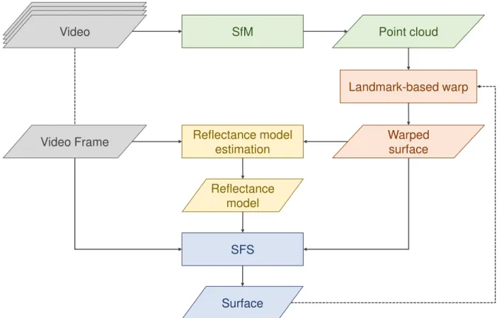
3.2 Method
Video Frame
Video Frame Video Frame Video Frame
Video SfM Point cloud
SFS
Warped surface
Reflectance model estimation
Reflectance model
Surface
Landmark-based warp
Figure 3.4: Diagram of the proposed iterative approach for dense surface reconstruction of a single video frame.
3.2.1 Initial PDE
Eq. (3.3) above models observed intensityIr(r(x, y), θi(x, y))for a generic, isotropic BRDF
with the assumption that the light source is colocated with the camera. In practice, the values of Ir are obtained directly from the input (grayscale) imageG,i.e.,Ir(r(x, y), θi(x, y)) = G(x, y).
Joining Eq. (3.3) with Eqs. (3.5) and (3.8) and multiplying byr2, we have
(x2+y2+ 1)Ge2v −IiAcos(θi)BRDF(θi) = 0 (3.9)
(notee2v = z2). The dependence ofG,v, andθ
i on(x, y)is implied. The ultimate goal of the
following formulation is to solve for log-depthv(and from this, to derive the depthz) at each point in the image.
To simplify the notation, denoteL(x, y) = (x2+y2+ 1)G(x, y). Also, at each point(x, y), let
η(vx, vy) = IiAcos(θi)BRDF(θi). (Recall thatθican itself be expressed as a function ofvx andvy,
according to Eq. (3.8).) Using these substitutions and adopting appropriate boundary conditions to handle the image domain, we can write Eq. (3.9) as a static PDE ofvand its derivatives:
Le2v−η(v
x, vy) = 0, (x, y)∈Ω
v(x, y) = ψ(x, y), (x, y)∈∂Ω,
(3.10)
where the dependence ofηandLonxandyis implied. ψ(x, y)defines boundary conditions for the PDE.
3.2.2 Regularization
feature point(xk, yk)with estimated depthzk, we would requirev(xk, yk) = lnzk. However, such
constraints are ineffective in the PDE formulation, as they have no effect on the solution outside of that 2D location (Horovitz and Kiryati, 2004). The 3D point cloud acquired via SfM can also potentially yield noisy or outlier depth measurements, especially for scenes where the camera motion is small, which results in larger depth uncertainty for 3D triangulation. Moreover, even minor surface deformations can further degrade triangulation accuracy in live endoscopy. Thus, it is inadvisable to fix the depths estimated by SfM to exact values.
Instead, assume there exists a current estimatefest(x, y)of the surface viewed by the camera. In
the iterative scheme introduced below,fest(x, y)is a warped surface that passes near the 3D SfM
points. A simple regularization is added to the SfS PDE (Eq. (3.10)) that constrains the solution to be similar to the estimated surface in high-confidence regions (i.e. regions where the warped surface agrees with the SfM feature points). This is captured in the following energy function:
E(v) =E0(v) +
Z
Ω
λ 2(e
v −z
est)
2
dx. (3.11)
The termE0(v)denotes an energy functional effecting the original SfS PDE,i.e., ∂E∂v0 =Le2v−
η(vx, vy). The function zest(x, y) is the (fixed) depth of the existing surface at a given image
coordinate, and the parameterλ(x, y) ≥ 0controls the influence of the regularization term. An approach for calculatingλ(x, y)is defined below, when the final iterative algorithm is introduced. The squared loss term is a design choice, of course; in principle, robust choices such as the absolute difference could be adopted, to help alleviate gross errors in the current estimated surface.
The minimum ofE(v)is a new PDE:
∂E ∂v =Le
2v
−η(vx, vy) +λ(ev−zest)ev
!
The associated PDE with boundary conditions can be written as
(L+λ)e2v−λz
estev−η(vx, vy) = 0 (x, y)∈Ω
v(x, y) = ψ(x, y). (x, y)∈∂Ω.
(3.13)
3.2.3 Solving the PDE
Ahmed and Farag (2006) introduced a fast-sweeping method for SfS with the Oren-Nayar reflectance model (Oren and Nayar, 1994), itself based on a method by Kao et al. (2004), that can be used to solve PDEs like the regularized equation introduced above. I adopt this solving scheme here and outline how it can be extended to any general 1D reflectance model. Their approach uses the Lax-Friedrichs (LF) Hamiltonian, which provides an artificial viscosity approximation for solving static Hamiltonian-Jacobi equations,i.e., functions of the formH(x,∇v(x)) = R(x). The LF Hamiltonian is advantageous in that it is able to handle non-convex, complex Hamiltonian equations. While time-independent PDEs like Eq. (3.13) are not Hamiltonian equations due to the reliance of the variablev, Ahmed and Farag (2006) demonstrated that the LF Hamiltonian can be effectively applied to these types of equations.
3.2.3.1 Discretization
Before explaining the LF solving scheme, it is necessary to first introduce some numerics that underlie the approximation of the PDE. Let the image space be uniformly discretized into columns xiand rowsyj with grid spacing∆xand∆y. Letvi,j be the log-depth at position(xi, yj). Denoting
p= ∂v
∂x andq = ∂v
∂y, the forward- and backward-difference approximations ofpcan be represented
as
p+i,j = 1
∆x(vi+1,j−vi,j) and p
−
i,j =
1
respectively, and similarly forq. Let
¯ pi,j =
p+i,j +p−i,j
2 and q¯=
qi,j+ +q−i,j
2 (3.15)
be the average of the finite differences, and let
¯
vxi,j = vi+1,j +vi−1,j
2 and v¯
y i,j =
vi,j+1+vi,j−1
2 (3.16)
be the average value of the grid elements adjacent tovi,j.
3.2.3.2 Applying the Lax-Friedrichs Hamiltonian
Consider a general static Hamiltonian equation H(x, y, p = vx, q = vy) = 0. To obtain
a solution of v that approximately satisfies this equation, the 2D Lax-Friedrichs Hamiltonian introduces artificial viscosity terms
σi,jx ≥ max p∈[A,B],q
∂H
∂p (xi, yj, p, q)
and σyi,j ≥ max
q∈[C,D],p
∂H
∂q (xi, yj, p, q)
(3.17)
that ensure stability of the solution scheme (Kao et al., 2004; Shu, 2007). In a global LF scheme, [A, B]and[C, D]cover the entire valid range ofpandq, respectively, whereas in a local LF scheme, [A, B] = [min(p+i,j, p−i,j),max(p+i,j, p−i,j)] and [C, D] = [min(q+i,j, q−i,j),max(qi,j+, qi,j−)]. See below for further discussion on these parameters. Implicitly assuming the dependence on (xi, yj), the
functionH is approximated by the LF Hamiltonian:
˜
HLF(vi,j, vi+1,j, vi−1,j, vi,j+1, vi,j−1) = H(¯pi,j,q¯i,j)+
σx i,j
∆x vi,j −¯v
x i,j +σ y i,j
∆y vi,j −¯v
y i,j
, (3.18)
where the “bar” terms are from Eqs. (3.15) and (3.16), above.1
1This is a slightly unconventional way of expressing the LF Hamiltonian, which is typically written with artificial
viscosity terms−σx
2(p +
−p−)and−σy
2 (q +
As mentioned before, Ahmed and Farag (2006) demonstrated that this augmentation can be applied to more general equations like the original PDE in Eq. (3.13). The PDE becomes
(L+λ)e2vi,j −λz
estevi,j −η(¯pi,j,q¯i,j) +
σx
i,j
∆x + σi,jy ∆y
vi,j −
σx i,j
∆x¯v
x i,j −
σi,jy ∆y¯v
y
i,j = 0, (3.19)
plus appropriate boundary conditions that are detailed below. In a similar vein to Ahmed and Farag (2006), we can solve for the new value ofvi,j using Newton’s root-finding method,i.e., expressing
the left side of the above equation in a generic form of
g(v) =ae2v−bev+cv−d, g′(v) = 2ae2v −bev+c, (3.20)
the value ofvis updated using the following equation until the solutiong(v) = 0is satisfied:
v :=v− g(v)
g′(v). (3.21)
3.2.3.3 Fast Sweeping Scheme and Boundary Conditions
Kao et al. (2004) and Ahmed and Farag (2006) both outline the general algorithm for fast sweeping using the LF Hamiltonian, so I detail it on a high level, here. For initialization, the log-depth valuesvi,j are set to a large positive constant. The algorithm then proceeds to iteratively
update these values to progressively closer depths, applying Eq. (3.21) to determine the new value for one vi,j at a time. Stable updates are maintained using diagonal “sweeps” that alternative
between bottom left to top right, bottom right to top left, top left to bottom right, and top right to bottom left. For example, in the top-left-to-bottom-right sweep, the value of a generalvi,j will be
updated using values ofvi−1,jandvi,j−1 that have already been updated in the current sweep and
values ofvi+1,jandvi,j+1that have yet to be updated. Updates are applied until the total change in
To avoid computational catastrophe on the borders of the image, where the 4-neighborhood structure needed for H˜LF is unavailable, Kao et al. (2004) propose boundary conditions to be
applied on the edge of the image after every sweep. On the left border (and similarly for other three borders), their approach computes a new value ofv0,junder two possible conditions: p+1,j =p−1,j
andp+1,j =−p−1,j. If the maximum of these new values is smaller than the current value ofv0,j,v0,j
is updated to this smaller value.
In practice, I have found that taking the maximum of the two values can often lead the solution to exhibit strongly incorrect geometry near the boundary, at least for endoscopic applications (Fig. 3.5). This is due to the ground-truth surface (which is essentially a tube) near the image boundary often being very oblique w.r.t the camera’s viewing direction. Instead, taking theminimumof the two values seems to offer generally better results — with an additional constraint that the surface slope at the boundary is not too large. The boundary condition is thus applied on the left border using
v0,j := min(max(min(2v1,j−v2,j, v2,j), v1,j−∆maxv )v0,j), (3.22)
where∆max
v is the change invcorresponding to a maximum allowed incident angle (e.g.,θi = 89.5◦)
at the image border. Similar boundary conditions are used for the other three image borders. Without the threshold on the maximum slope, sporadic artifacts can sometimes arise near the image boundaries due to specularities or dark regions (Fig. 3.5, third image). This value is somewhat sensitive – if the threshold is even85◦, I have found that the overall accuracy of the method can
suffer.
3.2.4 Computingσx
i,j andσ y
i,j for Arbitrary BRDFs
As mentioned previously,σx
i,j andσ y
i,j (Eq. (3.17)) can be chosen using either asglobal
param-eters or localparameters. The local LF scheme is generally preferred, since it exhibits smaller dissipation in the final LF solution due to the adaptive range in which the maximum is taken (Osher and Shu, 1991; Shu, 2007). In practice, however, values forσx
Figure 3.5: Compared to the ground-truth surface (left), the boundary conditions suggested by Kao et al. (2004) can lead to strong artifacts on the edges of the image for endoscopic applications (second from left). A minor change to these conditions can correct for this, although problematic artifacts can still occur (second from right), which can be alleviated by limiting the maximum surface slope along the image boundary (right).
at equality for both types of schemes, since the magnitude of the derivative must be evaluated over a range ofpandq, and at each pixel location. An alternative to finding this exact threshold is to instead find a reasonable upper bound that is relatively simple to compute. One way to approach this for SfS is to separate the 1D BRDF and surface representation — that is, treat the PDE as a function ofcos(θi)(cf. Eqs. (3.9) and (3.10)), and treatcos(θi)as a function ofx,y,p, andq(cf.
Eq. (3.8)).
To make this more clear, I next outline the computation forσx
i,j. The valueσ y
i,j has a similar
formulation. In the following, I useθ =θifor the incident light angle to avoid confusion with(i, j)
subscripts.
First, note that for the regularized SfS PDE H (Eq. 3.13), ∂H∂p = ∂η∂p, where again p = vx.
In Section 3.2.1, η(p, q) was formulated as a 2D function (ignoring the dependence on x and y) to clarify the PDE formulation; however, we can equivalently express it as a 1D function,
˜
have at pixel location(xi, yj)that
max
p∈[A,B],q
∂H
∂p (xi, yj, vi,j, p, q)
= max
p∈[A,B],q
∂η ∂cos(θ) ∂cos(θ)
∂p (xi, yj, p, q)
≤ max
p∈[A,B],q
∂η
∂cos(θ)(xi, yj, p, q)
max
p∈[A,B],q
∂cos(θ)
∂p (xi, yj, p, q)
≤ max
cos(θ)∈(0,Tx i,j]
∂η˜
∂cos(θ)(cos(θ))
max p,q ∂cos(θ)
∂p (xi, yj, p, q)
, (3.23) whereTx
i,j is the largest possible value ofcos(θ)givenp+i,j andp
−
i,j, for any value ofq. The lower
bound of zero arises because an arbitrarily large value ofqcan be chosen; the upper bound ofTx i,j
arises because the maximum value ofcos(θ)decreases monotonically withp. For the right term, I have found that a global range for|∂cos(θ)∂p |is more tractable to work with, so I have adopted it, here.
It turns out that bothTx
i,jand the second maximum are computable in closed form (see Appendix
A). The first maximum may or may not be easy to compute – for example, if the underlying BRDF model is assumed to be Lambertian, it is a constant, whereas other models may require a search of the entire range. For purposes of a general and efficient implementation, I use numeric differentiation to approximate
∂η ∂cos(θ)
for values of cos(θ)from 0 to 1, and I maintain a lookup
table of the cumulative maximum for any value ofTx i,j.
3.2.5 Image-weighted Finite Differences
The artificial viscosity introduced by the Lax-Friedrichs Hamiltonian can be quite dissipative (Osher and Fedkiw, 2003), meaning solution schemes involving the Hamiltonian will poorly approximate functions along discontinuities. For a surface function f(x, y) (Eq. (3.4)), such discontinuities occur along self-occlusion boundaries of the surface in the image. To address this issue, I propose a simple image-intensity-based weighting scheme forp¯i,j,q¯i,j,¯vi,jx , and¯v
y i,j that
More explicitly, consider the observed radianceIi,j for a pixel(xi, yj)normalized to the range
[0,1]. Define wxi,j± = exp
−Ii,j−Ii±1,j
σI
2
, and similarlywyi,j±. The parameterσI defines the
spread of the weighting, with smaller values placing a higher penalty on intensity differences (σI = 0.1for the experiments later in this chapter). The valuesp¯i,j andq¯i,j introduced above are
now redefined asp¯i,j = wx+1 i,j+w
x−
i,j
wx+i,jp+i,j+wi,jx−p−i,j
andq¯i,j = wy+1 i,j+w
y−
i,j
wi,jy+qi,j+ +wyi,j−qi,j−
. A similar weighting is applied for¯vx
i,j andv¯ y i,j.
3.2.6 Reflectance Model
The choice of reflectance model is key to achieving realistic SfS reconstructions. In the case of nasopharyngoscopy, the underlying surface consists of throat tissue covered by a thin layer of saliva. While throat tissue is generally Lambertian, meaning that reflected light intensity is a direct function ofcosθi (and thus the BRDF is a constant related to the surface albedo), the extra salivary coating
induces superficial reflections that significantly alter the overall reflectivity. Since these non-diffuse effects are signficantly different from those modeled by existing non-Lambertian SfS approaches (Ahmed and Farag, 2006; Vogel et al., 2009), I propose to instead model the saliva/tissue reflectance using a general basis for 1D BRDFs.
3.2.6.1 BRDF Basis
The proposed reflectance model is based on the set of BRDF basis functions introduced by Koenderink et al. (1996). These functions form a complete, orthonormal basis on the half-sphere derived via a mapping from the Zernike polynomials, which are defined on the unit disk. As-suming Helmholtz’s reciprocity2 and surface isotropy, the basis consists of a set of functions
Sl
nm(θi, θr,∆φir), where ∆φir =|φi−φr|,0 ≤ l ≤ m ≤ n ≤ N, and the quantites(n−l)and 2
(m−l)are even. N represents the order of the BRDF. The basis functions have the form
Snml (θi, θr,∆φir) = Θln(θi)Θlm(θr) + Θlm(θi)Θln(θr)
cosl∆φir. (3.24)
Here,Θb
a(θ)is proportional to the radial functionRba
√
2 sin θ2
, which itself takes the form of a terminating hypergeometric series. Θb
a(θ)can thus be expressed as a polynomial ofsin(θ2)with
powers ranging frombtoa:
Θba(θ) =
a
X
k=b
cksink
θ 2
, (3.25)
where the coefficientsck are proportional to coefficients of the terminating hypergeometric series.
(The exact value of ck is not important for this exposition, as it will later be combined with
parameters for the BRDF.) The final BRDF is a sum of the individual basis functions:
BRDF(θi, θr,∆φir) =
X
nml
cnmlSnml (θi, θr,∆φir), (3.26)
where the coefficientscnmlare parameters that dictate the specific BRDF.
3.2.6.2 Proposed Reflectance Model
The BRDF basis of Koenderink et al. (1996) can be adapted to produce a multi-lobe reflectance model for camera-centric SfS. First, taking the light source to be at the camera center, we have θi =θrand∆φir = 0. Combining with Eqs. (3.24) and (3.25), this gives
Snml (θi) = 2Θln(θi)Θlm(θi)
= 2
n
X
k=l
cksink
θ 2
! m
X
k=l
cksink
θ 2 ! = 2
c2l sin2l
θ 2
+ 2clcl+1sin2l+1
θ 2 +· · · = nm X k=2l
c′ksink