Variable Selection for Models with Missing Data
Ramon Israel Garcia
A dissertation submitted to the faculty of the University of North Carolina at Chapel Hill in partial fulfillment of the requirements for the degree of Doctor of Philosophy in the Department of Biostatistics.
Chapel Hill 2009
Approved by:
Joseph G. Ibrahim, Advisor
Hongtu Zhu, Advisor
R. Woodrow Setzer, Reader
Wei Sun, Reader
c
2009
Abstract
RAMON ISRAEL GARCIA: Variable Selection for Models with Missing Data.
(Under the direction of Joseph G. Ibrahim and Hongtu Zhu.)
Acknowledgments
Preface
About half way through the completion of my thesis, I started to think about the reason why I started to get my PhD in the first place. When I could not come up with a good reason, I started to wonder why anyone would want to get their PhD. After thinking about it for a while, I determined that there are three reasons why any person would want to get their PhD: 1) genuine interest in the subject matter, 2) money, and 3) prestige. In thinking about these reasons and how they pertain to me, I realized: 1) that I enjoy studying biostatistics but there are other things I also enjoy studying, 2) that money cannot buy me happiness, and 3) the flattery of others is not important. And so, I had come to the realization that my original motivation for obtaining my PhD was not as important to me as it once was. It was at this moment in writing my thesis that, my productivity slowed down to a crawl.
Table of Contents
iv
List of Tables x
List of Abbreviations xi
1 Introduction and literature review 1
2 Variable selection for regression models with missing data 4
2.1 Introduction . . . 4
2.2 Variable selection for regression models with missing data . . . 7
2.2.1 Model formulation . . . 7
2.3 Theoretical results . . . 13
2.4 Numerical studies . . . 16
2.4.1 Example 1: Simulation study . . . 16
2.4.2 Example 2: Melanoma data . . . 19
2.6 Appendix . . . 24
3 Variable selection in the cox regression model with covariates MAR 36 3.1 Introduction . . . 36
3.2 Variable selection for the Cox model with missing covariates . . . 39
3.2.1 Model formulation . . . 39
3.2.2 EM algorithm for maximizing the penalized likelihood . . . 41
3.2.3 Penalty parameter selection procedure . . . 44
3.3 Theoretical results . . . 46
3.4 Numerical studies . . . 49
3.4.1 Example 1: Simulation study . . . 49
3.4.2 Example 2: Veterans administration lung cancer data . . . 52
3.4.3 Example 3: Small lung cancer data . . . 53
3.5 Discussion . . . 54
3.6 Appendix . . . 56
4 Fixed and Random Effects Selection in Mixed Effects Models 70 4.1 Introduction . . . 70
4.2 Mixed effect selection for mixed effects models . . . 72
4.2.1 Model Formulation . . . 72
4.2.3 Penalty Parameter Selection Procedure . . . 76
4.3 Theoretical Results . . . 78
4.4 Numerical Studies . . . 81
4.4.1 Example 1: Simulation Study . . . 81
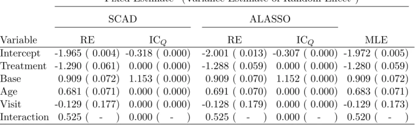
4.4.2 Example 2: Epilepsy Data . . . 84
4.5 Discussion . . . 87
4.6 Appendix . . . 88
List of Tables
2.1 Simulation results of linear regression model . . . 20
2.2 Estimates of Melanoma analysis . . . 22
2.3 Standard errors of penalized estimates . . . 34
3.1 Simulation results for Cox regression model . . . 52
3.2 Maximum penalized likelihood estimates of small lung cancer data . . . 54
3.3 Maximum penalized likelihood estimates of VA lung cancer data . . . . 69
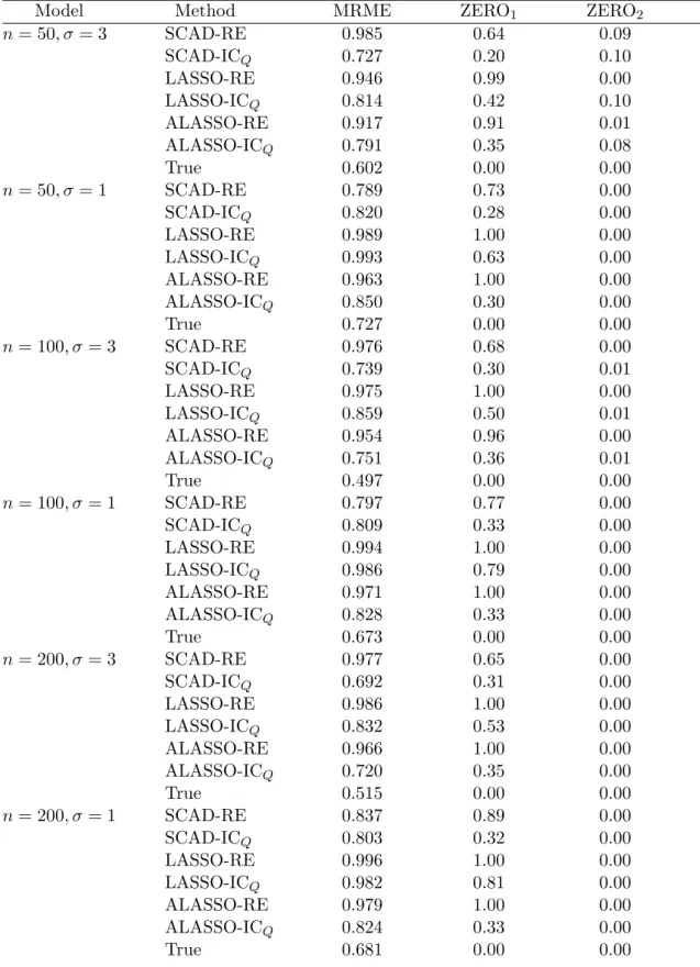
4.1 Simulation results of linear mixed effects models . . . 85
List of Abbreviations
AIC Akaike Information Criterion
ALASSO Adaptive Lasso
ALASSO-ICQ Maximum Penalized Likelihood Estimate using Adaptive Lasso Penalty Function and ICQ Penalty Estimate
ALASSO-RE Maximum Penalized Likelihood Estimate using Adaptive Lasso Penalty Function and Random Effects Penalty Estimate
BIC Bayesian Information Criterion
DIC Deviation Information Criterion
ECM Expectation Conditional Maximization
EM Expectation Maximization
GCV Generalized Cross Validation
LLA Local Linear Approximation
LQA Local Quadratic Approximation
MAR Missing at Random
MCMC Markov Chain Monte Carlo
ML Maximum Likelihood
MM Minorization-Maximization Algorithm
MME Mean Model Error
MPL Maximum Penalized Log-Likelihood
MRME Median Relative Model Error
NMAR Not Missing at Random
PL Penalized Likelihood
QOL Quality of Life
RE Random Effects Penalty Estimate
SCAD Smoothly Clipped Absolute Deviation
SCAD-ICQ Maximum Penalized Likelihood Estimate using SCAD Penalty Function and ICQ Penalty Estimate
SCAD-RE Maximum Penalized Likelihood Estimate using SCAD Penalty Function and Random Effects Penalty Estimate
SCLC Small Cell Lung Cancer
SIAS Simultaneous Impute and Select
SSVS Stochastic Search and Variable Selection
Chapter 1
Introduction and literature review
In the analysis of statistical models, one primary objective is to assess the impor-tance of certain prognostic factors such as age, gender, or race in predicting outcome. This objective is further complicated by the presence of missing data. Missing data are a common problem in various settings, including surveys, clinical trials, and longitu-dinal studies. Missing data may be present in the responses and/or covariates and in statistical models which include random effects or latent variables. Performing variable selection in statistical models for missing data problems raises several new statistical challenges, underscoring the need for methodological development.
An approach to variable selection is to use a selection procedure, such as forward or backward elimination, coupled with a selection criterion such as AIC and BIC based on the observed data log-likelihood, to select a small subset of ‘covariates’ that best predicts the outcome of interest. Such an approach, however, becomes infeasable even in the absence of missing data, because of the large number of possible models (Breimann, 1996; Fan and Li, 2001; Fan and Li, 2002).
Smoothly Clipped Absolute Deviation penalty (SCAD) (Fan and Li, 2001), least an-gle regression (Efron et al., 2003), Adaptive Lasso (ALASSO) (Zou, 2006), and group LASSO (Yuan and Li, 2006; Meier et al., 2008). These methods have been successfully applied to generalized linear models and robust linear regression (Fan and Li, 2001; Fan and Peng, 2004), semiparametric models including Cox’s proportional hazards model (Fan and Li, 2002, 2004; Cai et al., 2005; Zhang and Lu, 2007), and general regression models (Wang and Leng, 2007). Moreover, under an appropriate choice of the penalty parameter, the PL variable selection procedures can produce efficient estimates with or-acle properties (Fan and Li, 2001). The methods for selecting the penalty parameters consist of minimizing the penalty parameter with respect to some criterion. Com-monly used criteria include the generalized crossvalidation (GCV) and the Bayesian Information Criterion (BIC). It has been shown that BIC can identify the true model consistently, whereas GCV cannot (Wang et al. 2007; Wang and Leng, 2007). Ideally, one would like to use a criterion which results in appropriate choices of the penalty parameter so that the penalized likelihood estimates can possess oracle properties.
Thus, it is also critical to develop a new penalty selection criterion, which is easy-to-compute, for missing data problems. However, to the best of our knowledge, a general and easy-to-compute penalty and variable selection procedure is not currently available for missing data problems.
The aim of this dissertation is to develop a variable selection and a joint fixed and random effects selection procedure along with a penalty selection procedure using the SCAD and ALASSO penalties for a class of statistical models in missing data problems, including generalized linear models with missing covariates and/or responses, random effects models, latent variable models, and Cox’s proportional hazards model. We reformulate the penalty parameters in the SCAD and ALASSO as a hyperparameter of the regression coefficients, and then we use the EM algorithm to simultaneously optimize the penalized likelihood function and estimate the penalty parameters. In addition, we also develop an alternative method based on optimizing a new criterion, called the ICQ criterion (Ibrahim, Zhu and Tang, 2008), to select penalty parameters. The variable selection and penalty selection procedures developed here are very general and can be applied to numerous situations involving missing data and/or random effects and latent variables. Under some regularity conditions, we establish the asymptotic properties (e.g., oracle properties) of the maximum penalized likelihood estimator and the consistency of the ICQ based penalty selection procedure.
Chapter 2
Variable selection for regression
models with missing data
2.1
Introduction
penalized likelihood estimates can possess oracle properties. However, to the best of our knowledge, a general and easy-to-compute penalty and variable selection procedure is not currently available for missing data problems.
Missing data are a common problem in various settings, including surveys, clini-cal trials, and longitudinal studies. Responses and/or covariates may be missing, and statistical models for handling the missing data often depend on the missing data mech-anism, such as data not missing at random (NMAR), also referred to as nonignorable missingness. For example, when there are NMAR covariates, one must specify both the covariate distribution and the missing data mechanism in the likelihood function. These additional distributions bring additional parameters into the model, that need to be taken into consideration in model selection. It is common to use some model selec-tion criterion, such as AIC and BIC, based on the observed data log-likelihood to select a small set of variables. For instance, one might use AIC (or BIC) to select a small subset of ‘covariates’ that best predicts the outcome of interest. However, even in the absence of missing data, model selection criteria, such as AIC, can become infeasible for variable selection in linear regression models with a large number of covariates (Fan and Li (2001), Fan and Li (2002)). More discussion on the drawbacks of best subset selection can be found in Fan and Li (2001).
variables and calculate their estimates. Furthermore, computing the GCV and BIC to select the penalty parameter also requires computing the intractable likelihood func-tion and running an optimizafunc-tion algorithm for each penalty parameter, which can be computationally intensive for missing data problems. Thus, it is also critical to develop a new penalty selection criterion, that is easy-to-compute, in missing data problems.
The aim of this paper is to develop variable selection and penalty selection proce-dures, along with the SCAD and ALASSO penalties, for a class of statistical models in missing data problems, including generalized linear models with missing covariates and/or responses, random effects models, and latent variable models. We reformulate the penalty parameters in the SCAD and ALASSO as a hyperparameter in the model, and then we use the EM algorithm to simultaneously optimize the penalized likelihood function and estimate the penalty parameters. In addition, we also develop an alter-native method based on optimizing a new criterion, which we call the ICQ criterion, to select penalty parameters. The variable selection and penalty selection procedures developed here are very general and can be applied to numerous situations involving missing data and/or random effects and latent variables. Under some regularity condi-tions, we establish the asymptotic properties (e.g., oracle properties) of the penalized maximum likelihood estimator and the consistency of the ICQ-based penalty selection procedure.
2.4, a Melanoma dataset is analyzed with the proposed methodology. We conclude the paper with some discussion in Section 2.5.
2.2
Variable selection for regression models with
missing data
2.2.1
Model formulation
For notational simplicity, we focus on data with MAR or NMAR covariates; however, the methods developed below can be adapted to data with both missing responses and covariates (see Ibrahim, Chen, and Lipsitz (2001)). Suppose there are n independent observations (x1,z1, y1), . . . ,(xn,zn, yn), where yi is the response variable, zi is a q×1 vector of partially observed covariates, and xi is a (p−q)×1 vector of completely observed covariates. Let zm,i and zo,i, respectively, denote the missing and observed components ofzi. We use the q×1 random vector ri to indicate the missingness ofzi, where the kth componentrik = 1 when zik is observed and rik = 0 when zik is missing. We denote the complete and observed data of subject i by Dc,i and Do,i, respectively, and the entire complete and observed data byDc and Do, respectively.
When the covariates are NMAR, the complete data likelihood is the product of the joint distribution of (yi,zi,ri) given xi, denoted by f(yi,zi,ri|xi), which is typically specified as a product of three conditional distributions as
f(Dc) = n
Y
i=1
f(yi,zi,ri|xi,η) = n
Y
i=1
f(yi|xi,zi,β,τ)f(zi|xi,α)f(ri|yi,xi,zi,ξ), (2.1)
the missing data mechanism, f(ri|yi,xi,zi,ξ), can be ignored from (2.1).
As in generalized linear models (see McCullagh and Nelder (1989, Chap. 2)), we assume that the conditional distribution ofyigiven (xi,zi), denoted byf(yi|xi,zi, β,τ), satisfies
E[yi|xi,zi;β,τ] =µi =g((xTi ,z T
i)β), (2.2)
where τ denotes the additional parameters in f(yi|xi,zi,β,τ), g(·) is a known link function, and β= (β1, . . . , βp)T is a p×1 vector of regression coefficients. In practice, it is common to assume thatyi given (xi,zi) belongs to the exponential family, such as the binomial, normal, Poisson, etc... (Little and Schluchter (1985), and Ibrahim and Lipsitz (1996)).
We model the missing-data mechanism for NMAR covariates according to either a joint log-linear model forf(ri|yi,xi,zi,ξ) or a product of a sequence of one dimensional conditionals as in Ibrahim, Chen, and Lipsitz (1999). Finally, we assume that the covariate distribution f(zi|xi,α) is also modeled via a sequence of one-dimensional conditional distributions as in and Ibrahim, Chen, and Lipsitz (1999), and is given by
f(zi|xi,α) = f(ziq|zi(q−1),· · ·, zi1,xi,α)× · · ·f(zi1|xi,α),
where we assume a specific order of conditioning.
2.2. Penalized Likelihood for Variable Selection
In the variable selection problem, our objective is to identify nonzero components ofβ in (2.2) and simultaneously estimate parameters, while accounting for the missing covariate data. We propose to maximize the penalized likelihood function given by
P(η|λ) = n
X
i=1
logf(Do,i|η)−n p
X
j=1
where λ = (λ1, . . . , λp)T, λj is the penalty parameter corresponding to the j-th re-gression coefficient βj, and f(Do,i|η) =
R
f(yi,zi,ri|xi,η)dzm,i is the observed-data log-likelihood function of the i-th observation. The penalty function, pλj(·), is a
non-negative, nondecreasing, and differentiable function on (0,∞) (Fan and Li (2001) and Zou (2006)). These properties ensure that the maximization of (2.3) results in esti-mates of β which are shrunk to zero if they are small. The corresponding covariates of the estimates that are zero are the insignificant predictors of the response variable, whereas the estimates that are not zero correspond to those covariates which are statis-tically significant predictors. By maximizing (2.3), one can select significant predictors and estimate parameters simultaneously while accounting for the missing data. This approach is in sharp contrast to stepwise selection procedures and Bayesian procedures (George and McCulloch (1993), and Yang, Belin, and Boscardin (2005)), that ignore stochastic errors inherited in the selection phase during estimation of the ‘best’ model (Fan and Li (2002)).
In (2.3), the parameters τ, α, and ξ are not penalized, so they are not shrunk to zero even though their actual values may be small. In this sense, variable selection does not occur in the covariate distribution and the missing data mechanism. However, care must be taken in the specification of these distributions since certain specifications can lead to identifiability issues for estimating α,ξ, and thusβ.
iteration, given η(s), the E step is to evaluate the Q−function given by
Qλ(η|η(s))
= E[logf(Dc|η)|Do,η(s)]−n p
X
j=1
pλj(|βj|) = Q(η|η
(s))−n p
X
j=1
pλj(|βj|)
= Q1(β,τ|η(s))−n p
X
j=1
pλj(|βj|) +Q2(α|η
(s)) +Q
3(ξ|η(s)) = Q1,λ(β,τ|η(s)) +Q2(α|η(s)) +Q3(ξ|η(s)),
where
Q3(ξ|η(s)) =
Z n X
i=1
log[f(ri|yi,xi,zi,ξ)]f(zm,i|xi,zo,i, yi,ri,η(s))dzm,i,
Q2(α|η(s)) =
Z n X
i=1
log[f(zi|xi,α)]f(zm,i|xi,zo,i, yi,ri,η(s))dzm,i,
Q1,λ(β,τ|η(s)) =
Z n X
i=1
log[f(yi|xi,zi,β,τ)]f(zm,i|xi,zo,i, yi,ri,η(s))dzm,i
−n
p
X
j=1
pλj(|βj|).
The M step of the algorithm involves maximizing Q1,λ(β,τ|η(s)), Q2(α|η(s)), and
Q3(ξ|η(s)), independently. Maximizing Qλ(η|η(s)) with respect to (α,τ,ξ) can be done using standard maximization algorithms, such as Newton-Raphson (Little and Schluchter (1985), and Ibrahim and Lipsitz (1996)). However, it is difficult to maxi-mizeQ1,λ(β,τ(s)|η(s)) with respect toβ, because it is nondifferentiable and nonconcave (Zou and Li, 2007).
To maximizeQ1,λ(β,τ(s)|η(s)) with respect toβ, we approximateQ1(β,τ(s)|η(s)) us-ing a second order Taylor’s series expansion centered atβ(s). Using this approximation,
the local quadratic approximation algorithm (LQA) (Fan and Li (2001)), the best con-vex minorization-maximization algorithm (MM) (Hunter and Li (2005)), and the local linear approximation algorithm (LLA) (Zou and Li (2007)). We use the local linear approximation method to maximizeQ1,λ(β,τ(s)|η(s)), because it has been shown to re-duce the computational cost of maximizing penalized likelihoods (Zou and Li (2007)). Even though an approximation is used forQ1,λ(β,τ(s)|η(s)), the maximizer of this func-tion, denotedβ(s+1), will behave such that Q
1,λ(β(s+1),τ(s)|η(s))≥Q1,λ(β(s),τ(s)|η(s)). Therefore, using the ECM algorithm (Meng and Rubin (1993)), we can obtain aη(s+1) such that Qλ(η(s+1)|η(s))≥ Qλ(η(s)|η(s)), rather than directly maximizing Qλ(η|η(s)). We iterate this process until it converges to a value and denote the value at convergence by ˆηλ. Thus, ˆηλ maximizes the penalized observed data log-likelihood.
2.3. Penalty Selection Procedure
To ensure thatηbλ has oracle properties, the penalty parameterλhas to be appropri-ately selected. Two commonly used criteria for selecting the penalty parameter include the GCV and BIC criteria. These criteria cannot be easily computed in the presence of missing data because they are often functions of the missing data, and thus involve intractable integrals. Moreover, it has been shown that even for the linear model, the GCV can lead to significant overfitting (Wang, Li and Tsai (2007)).
We propose two methods to select the penalty parameter: an ICQ criterion and a random effects penalty estimation method. The ICQ criterion selects the optimalλ by minimizing
ICQ(λ) =−2Q(ηbλ|ηb0) + ˆcn(ηbλ),
whereηb0 = argmax
η
Pn
criterion; alternatively, we obtain a BIC-type criterion when ˆcn(η) = dim(η)×logn. Moreover, in the absence of missing data, we just obtain the usual AIC or BIC criteria. In practice, it is easy to compute ICQ for different λ because we only need samples fromf(zm,i|yi,xi,zo,i,ηb0) to approximate Q(ηbλ|ηb0) at each λ.
The random effects penalty estimator is calculated under the assumption that the regression coefficientsβ are distributed as random effects in a hierarchical model. The parameter λ can be regarded as a parameter in the distribution of β, denoted by
f(β|λ, n). Then, λ can be estimated by maximizing the marginal likelihood given by
Z n Y
i=1
Z
f(yi,zi,ri|xi,η)f(β|λ, n)dzm,idβ = n
Y
i=1
Z
f(Do,i|η)f(β|λ, n)dβ, (2.4)
where
f(β|λ, n) = p
Y
j=1
exp(−npλj(|βj|))/[C(λj, n)]
p, (2.5)
in which C(λj, n) is the normalizing constant of exp(−npλj(|βj|)). The resulting
es-timate of λ, denoted by ˆλRE, from the maximization of (2.4) is the random effects penalty estimator. The EM algorithm can be used to calculate ˆλRE by treating the regression coefficients as missing data in the marginal likelihood.
We consider the SCAD and ALASSO penalties as follows. For ALASSO,
pλj(|βj|) =λj|βj|
for j = 1,· · · , p. Typical values chosen are λj =λ0|βˆj|−γ, where ˆβj is the unpenalized ML estimate andγ >0 is a pre-specified positive scalar. In contrast, the SCAD penalty (Fan and Li, 2001) is a nonconcave function defined by pλ(0) = 0 and for|β|>0,
p0λ(|β|) =λ1(|β| ≤λ) + (aλ− |β|)+
where 1(·) denotes the indicator function,t+ denotes the positive part oft, anda= 3.7. Because the function exp(−npλ(|β|)) for the SCAD penalty is not proper, we use a truncated version ofpλ(|β|) to define the density f(β|λ, n). For SCAD, we have
f(β|λ, n)C(λ, n) =
exp(−nλ|β|), |β|< λ,
exp(n[|β|2−2aλ|β|+λ2]/[2(a−1)]), λ≤ |β| ≤aλ,
exp(−n(a+ 1)λ2/2), aλ≤ |β| ≤ |β|,¯
0, |β|>|β|,¯
where ¯β is arbitrarily large. For the ALASSO penalty, this truncation is not necessary because exp(−npλ(|β|)) is proper.
A closed form expression of ˆλRE is unavailable for both the ALASSO and SCAD penalties. But for the ALASSO penalty, a closed form expression of the conditional maximizer of the log-likelihood function with respect to λ is available. This allows a straightforward implementation of the ECM algorithm to estimate λ. For the SCAD penalty, we use the Newton Raphson algorithm along with the ECM algorithm to estimate ˆλRE.
2.3
Theoretical results
In this section, we establish the asymptotic theory of penalized likelihood estimators and the consistency of the penalty selection procedure based on ICQ. Suppose that
β =
βT(1),β(2)T
T
, where β(1) and β(2) are, respectively, p1×1 and p2×1 subvectors. Let β∗ = β∗T
(1),β
∗T (2)
T
denote the true value of β. Without loss of generality, we assume thatβ(2)∗ = 0 and each of the components of β(1) is not zero.
Thus,SF ={1, . . . , p} and ST ={1, . . . , p1} denote the full and true covariate models, respectively. If S misses at least one important covariate, S 6⊃ ST, then S is referred to as an underfitted model; however, ifS 6⊃ ST, then S is an overfitted model. Assume that we only consider the selected covariates in S. The unpenalized and penalized ML estimates of η, denoted by ηbS and ηbλ, respectively, are
b
ηS = argmax
η:βj6=0,∀j∈S
n
X
i=1
logf(D0,i|η) andηbλ = argmax
η
P(η|λ)
whereηbSF =ηb0.
Theorem 1. Under assumptions (C1) - (C7) stated in the appendix, we have (i) ηbλ−η∗ = Op(n−1/2) as n → ∞, where ηbλ =
ˆ
βT (1)λ,βˆ
T (2)λ,τˆ
T
λ ,αˆTλ,ξˆTλ
T
and η∗
is the true value of η;
(ii) Sparsity: P( ˆβ(2)λ = 0)→1; (iii) Asymptotic normality: βˆT
(1)λ,τˆ T
λ ,αˆTλ,ξˆTλ
T
is asymptotically normal with mean and covariance defined in the appendix.
The proof of Theorem 1 is given in the appendix. It states that, by choosing the penaltyλ, there exists a root-n estimator ofη,ηbλ, and that this estimator must posses the sparsity property, i.e. ˆβ(2)λ = 0. Theorem 1(iii) hasηbλ asymptotically normal. An
expression for the asymptotic covariance matrix of ηbλ can be obtained using Louis’s method (Louis (1982)). These estimates are given in the appendix.
We investigate whether the ICQ(λ) criterion can consistently select the correct model. For each λ∈Rp+, ˆβ
λ naturally defines a candidate model Sλ ={j : ˆβλ,j 6= 0}. Generally, Sλ can be either underfitted, overfitted, or true. Therefore, Rp+ can be partitioned into three mutually exclusive regions Rp+u = {λ ∈ Rp+ : Sλ 6⊃ ST},
converging to one. To select a better model, we first calculate
dICQ(λ2,λ1) = ICQ(λ2)−ICQ(λ1) = 2Q(ηbλ1|ηb0)−cˆn(ηbλ1)−2Q(ηbλ2|ηb0) + ˆcn(ηbλ2).
We assume Sλ2 ⊃ Sλ1 and choose the model resulting from using the penalty value λ1
(i.e., Sλ1), if dICQ(λ2,λ1)≥0, otherwise we choose modelSλ2.
Define δQ(λ1,λ2) = E[Q(ηS∗λ1|η
∗)]− E[Q(η∗ Sλ2|η
∗)], and δ
c(λ2,λ1) = ˆcn(ηbλ2)−
ˆ
cn(ηbλ1), in which η ∗
S is defined in the appendix.
Theorem 2. Under assumptions (C1) - (C7) in the appendix, we have following results. (a) If for allSλ 6⊃ ST, lim inf
n δQ(λ,0)/n >0 andδc(λ,0) =op(n), then dICQ(λ,0)> 0 in probability for all Sλ 6⊃ ST.
(b) If E[Q(ηS∗
λ1|ηb0)]−E[Q(η
∗
Sλ2|ηb0)] = Op(n
1/2) and Q(
b
ηλt|ηb0)−E[Q(η
∗
Sλt|ηb0)] =
Op(n1/2) for t= 1,2, then dICQ(λ2,λ1)>0 in probability asn−1/2δc(λ2,λ1) p
→ ∞. (c) If Q(ηbλ1|ηb0) −Q(ηbλ2|ηb0) = Op(1), then dICQ(λ2,λ1) > 0 in probability as
δc(λ2,λ1) p
→ ∞.
The proof of Theorem 2 is given in the appendix. Theorem 2 has some important implications. Theorem 2a shows that ICQ(λ) chooses all significant covariates with probability 1. Because S0 ⊂ Rpt ∪Rpo, the optimal model selected when minimizing ICQ(λ) will not select a λwithSλ 6⊃ ST because dICQ(λ,0)>0 in probability. There-fore, ICQ selects all significant covariates with probability tending to 1. Generally, the most commonly used ˆcn(η), such as 2dim(η), dim(η) log(n), andKlog log(n) (K >0), satisfy the condition δc(λ,0) = op(n). The condition lim inf
n n
−1δ
Q(λ,0) > 0 ensures that ICQ(λ) chooses a model with large E[Q(ηS∗|η∗)]. This condition is analogous to
underfit. Because n−1E[Q(η∗|η∗)]−n−1E[Q(η∗
S|η∗)] can be written as
n−1
n
X
i=1
logf(Do,i|η∗)−n−1 n
X
i=1
logf(Do,i|ηS∗)
+n−1E[H(η∗|η∗)]−n−1E[H(ηS∗|η∗)],
where
H(η|η1) =
Z n X
i=1
log[f(zm,i|xi,zo,i, yi,ri,η)]f(zm,i|xi,zo,i, yi,ri,η1)dzm,i,
it then follows from Jensen’s inequality thatn−1δ
Q(λ,0)≥0. Thus, if a modelS misses a significant covariate, it is reasonable to assume lim infnn−1δQ(λ,0) is greater than zero.
If λ1 and λ2 have the same averagen−1E[Q(ηS∗λ|η
∗)], that is,
lim infnn−1δQ(λ2,λ1) = 0, then Theorem 2 (b) and (c) indicate that ICQ(λ) picks out the smaller model Sλ1 when δc(λ2,λ1) increases to ∞ at a certain rate (e.g., log(n)).
For example, for the BIC-type criterion, δc(λ2,λ1) = [dim(ηbSλ2)−dim(ηbSλ1)] log(n)≥
log(n), since we assumeSλ2 ⊃ Sλ1. However, the AIC-type criterion ˆcn(η) = 2×dim(η)
does not satisfy this condition. Thus, similar to the standard AIC, ICQ with ˆcn(η) = 2×dim(η) tends to overfit.
2.4
Numerical studies
2.4.1
Example 1: Simulation study
effects and the ICQ penalty estimators, 2) compare the performance of the SCAD and ALASSO penalty functions, and 3) determine how the comparisons in 1) and 2) differ in the complete data and missing covariate settings.
To do this, we simulated datasets consisting of n observations from the model y = uTβ∗ +σwhere β∗ = (3,1.5,0,0,2,0,0,0)T and the components of u = (u1, . . . , u8), andare standard normal. The correlation betweenui anduj isρ|i−j|withρ=.5. This model was used in Fan and Li (2001). We considered three settings, (n = 40, σ = 3), (n = 40, σ = 1), and (n = 60, σ = 1). For each of them, two sets of 100 datasets were simulated, one with complete data and another with missing covariate data. For the datasets with missing data, the missing covariateszi = (u1i, u2i) were taken to be MAR and xi = (u3i, . . . , u8i) were completely observed. The covariate distribution is given by, [zi|xi]∼N2(µi,Σ) fori= 1, . . . , nwhereµi = (µ1i, µ2i),µsi =αs0+
P5
j=1αsjxisfor
s= 1,2 andΣis an unstructured 2×2 covariance matrix. The missing data mechanism used was f(ri1, ri2|yi,xi,φ) =f(ri1|ri2, yi,xi,φ1)f(ri2|yi,xi,φ2), where f(ri1|yi, xi,φ1) and f(ri2|ri1, yi, xi,φ2) are logistic regressions where the logistic regression parameters
φ1 and φ2 were selected such that 65% of the observations had complete data.
penalty we letλj =λ0, for allj, where in both casesλ0 was estimated using the penalty estimation methods.
In addition to the penalized estimates, the unpenalized ML estimate of the model selected by the simultaneously impute and select (SIAS) method of Yang, Belin, and Boscardin, (2005) was computed. SIAS implements the stochastic search variable se-lection (SSVS) method of George and McCulloch (1993) in the presence of missing covariates. SIAS is a fully Bayesian method which does not require model enumeration or computation of marginal likelihoods, so it may be easier to implement than other fully Bayesian methods. In the analysis of the datasets with no missing covariates, SIAS is equivalent to SSVS. Details of the implementation of SIAS are given in the appendix.
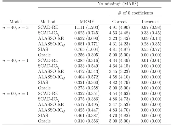
For each estimate ˆβλ, the model error, ME( ˆβλ) = ( ˆβλ−β∗)E(uuT)( ˆβλ−β∗), was computed and the ratio of the model error of the penalized ML estimate to that of the unpenalized ML estimate, ME( ˆβλ)/ME( ˆβ0), was computed. The median of these ratios over the 100 simulated datasets, denoted as MRME, is reported. The MRME of the true model, denoted as ‘oracle’, is also reported. In addition, the average number of zero coefficients correctly estimated to be zero and the average number of zero coefficients incorrectly estimated to be zero are reported. These are reported in the columns ‘Correct’ and ‘Incorrect’ respectively.
while values near the ‘oracle’ MRME value indicate optimal performance. The SCAD-RE performed poorly when the noise level was high, however, it is optimal when either the noise level is small or the sample size is large. The ALASSO-RE estimate had sub-stantial overfit since ‘Correct’ averaged significantly less than 5 indicating a tendency to not set insignificant coefficients to zero. The SIAS estimate performed as well as the unpenalized ML estimate when the noise level was large and covariates were missing, however it outperformed the ML estimate when either the noise level was high, the sample size was large, or all the covariates were fully observed. ‘Correct’ averages and ‘Incorrect’ averages that are both high indicate that the estimate is more likely to set coefficients to zero rather than not. This was the case with the SIAS and SCAD-RE estimates when the noise level was large. Comparing the analysis of no missing covari-ate data to the analysis with missing covaricovari-ate data shows that for all the estimcovari-ates, the estimation error increased, overfitting increased, and underfitting increased.
2.4.2
Example 2: Melanoma data
Table 2.1: Simulation results of linear regression model No missing1 (MAR2)
# of 0 coefficients
Model Method MRME Correct Incorrect
n= 40, σ = 3 SCAD-RE 1.111 (1.203) 4.91 (4.90) 0.97 (0.98) SCAD-ICQ 0.625 (0.745) 4.53 (4.48) 0.33 (0.45) ALASSO-RE 0.632 (0.690) 3.23 (3.42) 0.09 (0.13) ALASSO-ICQ 0.681 (0.771) 4.31 (4.23) 0.28 (0.35) SIAS 0.765 (1.004) 4.81 (4.87) 0.55 (0.77) Oracle 0.256 (0.305) 5.00 (5.00) 0.00 (0.00)
n= 40, σ = 1 SCAD-RE 0.285 (0.316) 4.34 (4.49) 0.01 (0.01) SCAD-ICQ 0.333 (0.549) 4.64 (4.15) 0.00 (0.00) ALASSO-RE 0.472 (0.543) 3.45 (3.23) 0.00 (0.00) ALASSO-ICQ 0.404 (0.572) 4.58 (4.10) 0.00 (0.00) SIAS 0.321 (0.360) 4.82 (4.79) 0.00 (0.00) Oracle 0.273 (0.258) 5.00 (5.00) 0.00 (0.00)
n= 60, σ = 1 SCAD-RE 0.322 (0.351) 4.54 (4.62) 0.00 (0.00) SCAD-ICQ 0.375 (0.386) 4.86 (4.73) 0.00 (0.00) ALASSO-RE 0.517 (0.495) 3.47 (3.53) 0.00 (0.00) ALASSO-ICQ 0.425 (0.447) 4.83 (4.70) 0.00 (0.00) SIAS 0.461 (0.387) 4.70 (4.82) 0.00 (0.00) Oracle 0.310 (0.356) 5.00 (5.00) 0.00 (0.00)
interferon and observation). From these six covariates, three had missing data while the rest of the covariates and the response variable were completely observed. The three covariates with missing data were Breslow thickness, size, and type. Logarithms of Breslow thickness and size were used in this analysis to achieve approximate normality of these covariates in the covariate distribution. The dataset had a total missing data fraction of 28.7%. The outcome variable, yi, was taken here to be binary, and was assigned a 1 if the patient had an overall survival greater than or equal to .55 years, and 0 otherwise. There were no censored cases that had an overall survival below .55 years.
and β = (β0, β1, . . . , β6). For the missing covariates, we assume they are MAR and have the covariate distribution
f(zi|xi;α) =f(zi3|zi1, zi2,xi;α3)f(zi1, zi2|xi;α1,α2)
for i= 1, . . . , n. Since xi is completely observed, it is conditioned on throughout. We take (zi1, zi2|xi) ∼ N2(µi,Σ), where µi = (µi1, µi2) and µis = αs0 +
P3
j=1αsjxij for
s = 1,2, i = 1, . . . , n, and Σ is an unstructured 2×2 covariance matrix. A logistic regression model was used for xi3 conditional on (zi1, zi2,xi). The same estimates as those computed in the simulations were computed. The statistical model used for the SIAS method is given in the appendix.
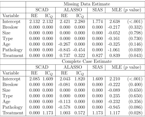
coefficient for treatment decreased from 1.117 in the complete case analysis to .839 in the missing data analysis. This change caused the SCAD-ICQ estimate to identify treatment as significant in the complete case analysis but not significant for the missing data analysis.
Table 2.2: Estimates of Melanoma analysis Missing Data Estimate
SCAD ALASSO SIAS MLE (p value)
Variable RE ICQ RE ICQ
Intercept 2.132 2.132 2.421 2.280 1.774 2.638 (<.001) Breslow 0.000 0.000 0.000 0.000 0.000 -0.217 (0.332) Size 0.000 0.000 0.000 0.000 0.000 -0.052 (0.798) Type 0.000 0.000 0.000 0.000 0.000 -0.161 (0.730) Age 0.000 0.000 -0.267 0.000 0.000 -0.325 (0.146) Pathology 0.000 0.000 -0.845 -0.454 0.000 -1.061 (0.039) Treatment 0.000 0.000 0.737 0.322 0.827 0.839 (0.043)
Complete Case Estimate
SCAD ALASSO SIAS MLE (p value)
Variable RE ICQ RE ICQ
Intercept 2.085 1.609 2.043 1.820 1.609 2.210 (<.001) Breslow 0.000 0.000 -0.081 0.000 0.000 -0.222 (0.400) Size 0.000 0.000 0.000 0.000 0.000 -0.089 (0.650) Type 0.000 0.000 0.000 0.000 0.000 0.235 (0.650) Age 0.000 0.000 -0.113 0.000 0.000 -0.232 (0.356) Pathology 0.000 0.000 -0.578 0.000 0.000 -0.945 (0.086) Treatment 0.000 1.173 1.003 0.572 1.173 1.117 (0.028)
2.5
Discussion
choice of ˆcn(η), the ICQ penalty estimate chooses all the significant predictors in prob-ability. Simulation results show that the SCAD penalty function with the random effects penalty estimate performs well when the noise level is small, whereas it per-forms poorly when the noise level is large. Overall, the SCAD performed better when it was used with the random effects penalty estimator whereas the ALASSO performed better when it was used with the ICQ criterion. The ALASSO penalty function with the random effects penalty estimate showed significant overfit in the finite sample sim-ulations and this overfit was also present in the Melanoma data analyses. The results of the Melanoma data analysis indicate that when predictors are not strongly significant, the results from penalized likelihood maximization may differ depending on the penalty functions and penalty selection methods which are used.
One of the disadvantages of penalized likelihood methods is that they do not provide a measure of model uncertainty, i.e. the probability of selecting each model in the model space. Other methods, such as Bayesian model averaging (Hoeting, Madigan, Raftery and Volinsky (1999) ), SIAS, or Bayesian methods in general provide estimates of posterior model probabilities. However, implementation of fully Bayesian methods can be difficult in many cases, since it requires specifying priors for all of the parameters in the response model, covariate distribution (and missing data mechanism under NMAR) which encompass all the models in the model space, as well as calculating marginal likelihoods and enumerating all the models in the model space. Alternatively, the SIAS method is easier to implement but, unlike penalized ML maximization, it does not give an estimate of the parameters of the ‘best’ model. Moreover, the results of the linear regression simulations indicated that the SCAD-RE estimate outperforms SIAS when either the noise level is small or the sample size is large.
such as generalized linear mixed models with nonignorable missing response and/or covariate data, semiparametric survival models with missing covariate data, such as the Cox model as well as frailty models, measurement error models, and partially linear models with missing covariates and/or responses. Throughout this paper, we made an implicit assumption that the response model does not depend on whether a covariate is observed or missing. That is, we have assumed a single response model for the covariate where it is missing or not. If we have a different response model for the observed and missing parts of the covariate, then the methods developed in this paper would not be able detect whether the missing part of a covariate is significant. In this scenario other statistical methods, such as propensity score methods, may be useful for handling this case (Kang and Schafer (2007)), but applying these methods to variable selection problems requires further developments both computationally and theoretically. We will formally investigate these issues in our future work.
2.6
Appendix
Assumptions for Proofs of Theorems 1 - 2 Even though the model `(η) = Pn
i=1`i(η) =
Pn
i=1logf(Do,i|η) may be misspeci-fied, White (1994) has shown that the unpenalized ML estimate converges to the value of η which minimizes E[Pn
i=1li(η)] =
Pn i=1
R
li(η)g(Do,i)dDo,i where g(·) is the true density. We denote the true value by η∗n = arg supηE[`(η)]. For simplicity, we fur-ther assume that E[∂ηli(η)] = 0 for all i and η∗ = η∗n, for all n. Similarly, we define
η∗Sn = argsupη:βj6=0,j∈SE[Q(η|η∗)] and let ηS∗n=ηS∗, for all n.
The following assumptions are needed to facilitate development of our methods, although they may not be the weakest possible conditions.
(C2) ηb0 →η∗ in probability.
(C3) For alli,li(η) is three-times continuously differentiable onΘandli(η),|∂jli(η)|2 and |∂j∂k∂lli(η)| are dominated by Bi(Do,i) for all j, k, l = 1,· · · , d where ∂j =
∂/∂ηj. We also require that the same smoothness condition also holds forh(Do,i;η) =
E[logf(zm,i|Do,i;η)|Do,i;η].
(C4) For each >0, there exists a finite K such that
sup n≥1
1
n
n
X
i=1
EBi(Do,i)1[Bi(Do,i)>K]
<
for all n.
(C5)
lim n→∞−
1
n
n
X
i=1
∂η2li(η∗) =A(η∗),
lim n→∞ 1 n n X i=1
∂ηli(η∗)∂ηli(η∗)T =B(η∗),
lim n→∞−
1
n
n
X
i=1
D20Q(ηS∗|η∗) = C(ηS∗|η∗),
lim n→∞ 1 n n X i=1
D10Q(ηS∗|η∗)D10Q(ηS∗|η∗)T =D(ηS∗|η∗),
whereA(η∗) andC(η∗S|η∗) are positive definite andDij denotes thei-th andj-th derivatives of the first and second component of theQ function respectively.
(C6) Define an = maxj
n
p0λ
jn(|β
∗
j|) :βj∗ 6= 0
o
, and bn = maxj
n
p00λ
jn(|β
∗
j|) :βj∗ 6= 0
o
.
1. maxj{λjn:βj∗ 6= 0}=op(1).
2. an =Op(n−1/2).
(C7) Define dn = minj{λjn :βj∗ = 0}.
1. For allj such thatβj∗ = 0, limn→∞λ−jn1lim infβ→0+p0λjn(β)>0 in probability.
2. n1/2d n
p
→ ∞.
Proof of Theorem 1a.
Given assumptions (C1) - (C6), then it follows from White (1994) that
n−1/2
n
X
i=1
∂ηli(η∗) D
→N(0,B(η∗)) (2.6)
and
n1/2(ηb0−η∗) D
→N 0,A(η∗)−1B(η∗)A(η∗)−1
. (2.7)
To showηbλ is a
√
n-consistent maximizer ofη∗, it is enough to show that
P sup
||u||=C
(
`(η∗+n−1/2u)−n
p
X
j=1
pλjn(|β
∗
j +n
−1/2u j|)
)
−`(η∗) +n
p
X
j=1
pλjn(|β
∗
j|)<0
!
converges to 1 for large C, since this implies there exists a local maximizer in the ball
expansion of the penalized likelihood function, we have
`(η∗+n−1/2u)−`(η∗)−n
p
X
j=1
pλjn(|β
∗
j +n
−1/2u j|) +n
p
X
j=1
pλjn(|β
∗
j|)
≤ `(η∗+n−1/2u)−`(η∗)−n
p1
X
j=1
pλjn(|β
∗
j +n
−1/2
uj|) +n p1
X
j=1
pλjn(|β
∗
j|)
= n−1/2uT∂η`(η∗)−
1 2u T −1 n∂ 2
η`(η
∗
)
u−n1/2
p1
X
j=1
h
p0λjn(|βj∗|)sgn(βj∗)uj
i −1 2 p1 X j=1 h
p00λjn(|βj∗|)u2j
i
+op(1)
≤ n−1/2uT∂η`(η∗)−
1 2u
TA(η∗
)u+√p1n1/2an||u1|| − 1
2|bn|||u1|| 2+o
p(1)
≤ n−1/2uT∂η`(η∗)−
1 2u
TA(η∗
)u+√p1n1/2an||u1||+op(1), (2.8)
where u= (uT1,uT2)T and u1 is a p1×1 vector. The second inequality in (2.8) follows because pλjn(0) = 0 and pλjn ≥ 0. The third inequality follows from condition (C5)
and the fact that Pp1
i=1|ui| ≤
√
p1(Ppi=11 u2i)1/2. The last inequality follows from (C6). Since the first and third terms in (2.8) are Op(1) by (2.6) and condition (C6) - 2, anduTA(η∗)uis bounded below by ||u||2×the smallest eigenvalue of A(η∗), then the
second term in (2.8) dominates the rest and all the terms can be made negative for large enoughC.
Proof of Theorem 1b.
Suppose that the conditions of Theorem 1a hold, and there exists an, ηbλ, which is a √n-consistent estimator of η∗. It suffices to show that for large n, the gradient of the penalized log likelihood function evaluated atηbλ, such that||ηbλ−η
∗||=O
penalized log likelihood function about η∗, we have
0=n−1/2
∂η`(ηbλ)−n ∂η ( p
X
j=1
pλjn(|βj|)
)
η=ηbλ
= n−1/2∂η`(η∗)−n1/2(ηbλ−η
∗ )T −1 n∂ 2
η`(η
∗
)
+Op(n−1)
−n1/2 ∂
η
( p X
j=1
pλjn(|βj|)
)
η=ηbλ = Op(1)−n1/2 ∂η
( p X
j=1
pλjn(|βjλ|)
)
η=ηbλ
(2.9)
where the last equality follows from n−1/2∂
η`(η∗) = n1/2(ηbλ −η
∗)T
−∂2
η`(η∗)/n
=
Op(1). Therefore, for j = p1 + 1, . . . p, the gradient with respect to βj of the second term of (2.9), is −sgn( ˆβj)n1/2λjn[λ−jn1p0λjn(|
ˆ
βj|)]. Since ||βˆ(2)λ|| =op(1), λ−jn1p0λjn(|
ˆ
βj|) is greater than zero for largen, it follows that (2.9) is dominated by the term−sgn( ˆβj)n1/2dn. Sincen1/2d
n p
→ ∞, it must be the case that ˆβjλ = 0 for j =p1+ 1, . . . , p, otherwise the gradient could be made large in absolute value and could not possibly be equal to zero.
Proof of Theorem 1c.
Given conditions (C1) - (C7), Theorems 1a and 1b apply. Thus, there exists a ˆ
βλ =
ˆ
βT (1)λ,0
TT, and ˆη λ =
ˆ
βT
λ,τˆλT,αˆTλ,ξˆλT
T
which is a √n local maximizer of (6). Let β∗ = β∗T
(1),0
TT, γ∗ = β∗T (1),τ
∗T,α∗T,ξ∗TT, γ = βT (1),τ
T,αT,ξTT, ˆ
γλ =
ˆ
βT
(1)λ,τˆλT,αˆTλ,ξˆλT
T
, and ˜l(γ) = l((βT
A((βT (1),0,τ
T,αT,ξT)) and similiarly define ˜B. Let,
h1 β(1)
= (p0λ1(|β1|)sgn(|β1|), . . . , p0λp1(|βp1|)sgn(|βp1|))
T,
G1 β(1)
= diagp00λ1(|β1|), . . . , p00λp1(|βp1|)
,
h(γ∗) =
h1
β(1)∗
0
, G(γ
∗ ) = G1
β(1)∗ 0
0 0
,and
Σ(γ∗) =
h
˜
A(γ∗) +G(γ∗)
i−1
˜ B(γ∗)
h
˜
A(γ∗) +G(γ∗)
i−1
.
Then, using a Taylor’s series expansion, we have
0 = ∂γ˜l(bγλ)−n∂γ " p
X
j=1
pλj(|βλj|)
#
γ=γbλ = ∂γ˜l(γ∗)−nh(γ∗)−n(γbλ−γ
∗ )T −1 n∂ 2
γ˜l(γ
∗
) +G(γ∗)
+op(1)
= n−1/2∂γ˜l(γ∗)−n1/2h(γ∗)−n1/2(γbλ−γ
∗
)ThA(˜ γ∗) +G(γ∗)i+op(1),
which indicates
n1/2
b
γλ−γ∗+
h
˜
A(γ∗) +G(γ∗)i
−1 h(γ∗)
D
=n−1/2hA(˜ γ∗) +G(γ∗)i
−1
∂γl(γ∗),
and therefore
n1/2
b
γλ−γ∗+
h
˜
A(γ∗) +G(γ∗)i
−1 h(γ∗)
D
→N(0,Σ(γ∗)).
For the SCAD penalty with λjn = λn, if λn = op(1), n1/2λn p
→ ∞ and conditions (C1) - (C5) are satisfied, then the oracle properties of Theorem 1 hold. For the ALASSO penalty, withλjn=λn|βˆj|−1 where ˆβj is the unpenalized ML estimate,λn=Op(n−1/2),
nλn p
penalty function and specification ofλjn, the rates ofλjn which characterize the oracle properties, may be different.
Under the assumptions of Theorem 1 for the SCAD and ALASSO penalty functions, h(η∗)→0, therefore the asymptotic covariance matrix of ˆγλisn−1Σ(γ∗). Using Louis’s formula (Louis (1982)), an estimate ofΣ(γ∗) is,
Var(ˆγλ)≈n−1[ ˆA(ˆγλ) +G(ˆγλ)]−1B(ˆˆ γλ) [A(ˆγλ) +G(ˆγλ)]
−1
, (2.10)
where
˙
Qi(γ∗|γ∗) = ∂γ
Z
logf(Dc,i;γ,β(2) =0)f(zm,i|Do,i;γ∗,β(2) =0)dzm,i
γ=γ∗
,
ˆ
B(γ∗) = n−1
n
X
i=1 ˙
Qi(γ∗|γ∗) ˙Qi(γ∗|γ∗)T, ˙
Q(γ∗|γ∗) = ∂γQ((β(1),0,τ,α,ξ)|γ∗,β(2) =0)
γ=γ∗
¨
Q(γ∗|γ∗) = ∂γ2Q((β(1),0,τ,α,ξ)|γ∗,β(2) =0)
γ=γ∗,and
ˆ
A(γ∗) = −n−1Q¨(γ∗|
γ∗) +n−1Q˙(γ∗|η∗) ˙Q(γ∗|γ∗)T
−n−1E[(∂γlogf(Dc;γ,β(2) =0))⊕|Do;γ∗,β(2) =0]
γ=γ∗
wherev⊕ =vvT.
Proof of Theorem 2a.
To prove Theorem 2, we first show that for ηtn p
→ηt, t= 1,2,
Q(η1n|η2n)−Q(η1|η2) = op(n)
E[Q(η1n|η2n)]−E[Q(η1|η2)] = op(n)
Q(η1n|η2n)−E[Q(η1|η2)] = op(n). (2.11)
in probability to 0 for all η1,η2 ∈Θ. Furthermore, because conditions (C3) and (C4) satisfy the W-LIP assumption of Lemma 2 of Andrews (1992), we obtain the uniform continuity and stochastic continuity of E[Q(η1|η2)] and [Q(η1|η2)−E(Q(η1|η2))]/n respectively. Because the stochastic continuity and pointwise convergence properties satisfy the assumptions of Theorem 3 of Andrews (1992), we have
sup (η1,η2)∈Θ×Θ
1
n|Q(η1|η2)−E[Q(η1|η2)]|
p
→0, (2.12)
which implies (2.11).
We also need to show that the hypothetical estimator
¯
ηS = argsupη:βj6=0,j∈SQ(η|η ∗
)
is a √n-consistent estimator of ηS∗. To prove this, it is enough to show that
P
"
sup
||u||=C
Q(ηS∗ +n−1/2u|η∗)≤Q(ηS∗|η∗)
#
≥1−
for largeC, since this implies there exists a local maximizer in the ball{η+n−1/2u;||u|| ≤
C} and thus ||η¯S −ηS∗|| = Op(n−1/2). Taking a Taylor’s series expansion of the first component of the Qfunction, we have
Q(ηS∗ +n−1/2u|η∗)−Q(ηS∗|η∗) = n−1/2uTD10Q(η∗S|η∗)− 1
2u T
−1 nD
20Q(η∗ S|η∗)
u+op(1)
= n−1/2uTD10Q(η∗S|η∗)− 1
2u TC(η∗
S|η ∗
)u+op(1). (2.13)
(2.13) can be made negative for large enough C. Let ηeSλ = argsup
η:βj=0,j∈Sλ
Q(η|ηb0). Sinceηb0
p
→η∗ and ¯ηSλ
p
→η∗S
λ, we have
1
ndICQ(λ,0) =
1
n(ICQ(λ)−ICQ(0))
= 1
n [2Q(ηb0|ηb0)−2Q(ηbλ|ηb0) + ˆcn(ηbλ)−ˆcn(ηb0)]
≥ 2
n [Q(ηb0|ηb0)−Q(ηeSλ|ηb0)] +op(1)
= 2
n [Q(ηb0|ηb0)−Q(ηeSλ|η
∗
)] +op(1)
≥ 2
n [Q(ηb0|ηb0)−Q( ¯ηSλ|η
∗
)] +op(1)
= 2
nE[Q(η
∗|
η∗)]−EQ ηS∗
λ|η
∗
+op(1)
≥ 2
n S6⊃SminT
{E[Q(η∗|η∗)]−E[Q(ηS∗|η∗)]}+op(1),
where the second and fourth inequalities follow because Q(ηbλ|ηb0) ≤ Q(ηeSλ|ηb0) and
Q(ηeSλ|η
∗)≤Q( ¯η Sλ|η
∗) for all λ and the third and fifth equalities follow from (2.11).
Therefore, we have
P r
inf
λ∈Rpu
ICQ(λ)>ICQ(0)
→1,
Proof of Theorem 2b.
Under the assumptions of Theorem 2b, we have
n−1/2δQ(λ2,λ1) = n−1/2(ICQ(λ2)−ICQ(λ1)) = 2n−1/2(Q(ηbλ1|ηb0)−2Q(ηbλ2|ηb0)) +n
−1/2(ˆc(
b
ηλ2)−cˆ(ηbλ1))
= 2n−1/2Q(ηbλ1|ηb0)−E[Q(η
∗ Sλ1|ηb0)]
−2n−1/2Q(ηbλ2|ηb0)−E[Q(η
∗ Sλ2|ηb0)]
+2n−1/2
E[Q(η∗Sλ
2|ηb0)]−E[Q(η ∗ Sλ1|ηb0)]
+n−1/2δc(λ2,λ1) = Op(1) +n−1/2δc21
p
→ ∞.
Thus ICQ(λ2) > ICQ(λ1) in probability, which yields Theorem 2b. Proof of Theorem 2c is similar to that of Theorem 2b.
Statistical model for application of SIAS method to linear regression simu-lations.
To implement SIAS, we assume the response model isyi ∼N(uTiβ, σ2), the covariate distribution is ui ∼ N(µu,Σu) for i = 1, . . . , n and the missing covariates are MAR. For the prior distribution of all the parameters we assume
π(β,γ, σ2,µu,Σu) = p
Y
j=1
{π(βj|γj)π(γj)}π(σ2)π(µu|Σu)π(Σu)
where µu|Σu ∼ N8(0, δ−1Σu), Σu−1 ∼ Wishart(r,I8), σ−2 ∼ Gamma(ν/2, νω/2), βj ∼ (1−γj)N(0, t2j) + γjN(0, c2jt2j) and γj ∼ Bernoulli(1/2). The hyper-parameters were selected to reflect a lack of prior information on the parameters, i.e. δ = ν = ω =
.001, r = 8. For the values of tj and cj, we use those suggested by George and McCulloch (1993) where (σ2
βj/t
2
j, c2j) = (1,5),(1,10),(10,100),(10,300) and σβ2j was
We performed 5,000 simulations after a burn-in period of 5000 iterations. The pos-terior probability ofγwas calculated from the posterior simulations and the model with the highest probability was selected as the ‘best’ model. The results of (σ2
βj/t
2
j, c2j) = (1,10) are presented since it gives the best model with the highest posterior probability.
Simulation results evaluating performance of standard errors of penalized estimates for linear regression simulations
Table 2.3: Standard errors of penalized estimates
Method βˆ1 βˆ2 βˆ5
SD SDm SDmad SD SDm SDmad SD SDm SDmad SCAD-RE .138 .164 .042 .170 .187 .039 .160 .180 .039 SCAD-ICQ .141 .161 .039 .178 .180 .048 .163 .175 .038 ALASSO-RE .157 .161 .031 .183 .180 .035 .165 .173 .036 ALASSO-ICQ .139 .164 .039 .198 .185 .037 .166 .176 .038 Oracle .138 .155 .036 .179 .157 .040 .147 .139 .028
In order to test the accuracy of the asymptotic error formula (2.10), we estimated the standard errors of the significant coefficients,β1,β3, andβ5 for the linear regression model using n= 60, σ = 1 with the covariates missing at random. The median of the absolute deviations |βˆjλ −βj∗| divided by .6745, denoted by SD, of the 100 penalized estimates can be regarded as the true standard error. The median of the estimated standard errors is denoted as SDm. The median absolute deviation error divided by .6745, denoted SDmad, measures the overall performance of the standard error formula. The results, which are presented in Table 2.3, indicate that the standard error estimate does a good job of estimating the true standard error. All of the SDmad values were less than .05.
Statistical model for application of SIAS method to Melanoma data
γi = (1, zi, xi)Tβ, andβ = (β0, β1, . . . , β6)T. We assume the covariates are MAR with the following covariate distribution
f(zi|xi;α) =f(zi3|zi1, zi2,xi;α3)f(zi1, zi2|xi;α1,α2)
fori= 1, . . . , n. Since xi are completely observed, they are conditioned on throughout. We take a (zi1, zi2|xi)∼N2(µi,Σ), whereµi = (µi1, µi2) andµis =αs0+
P3
j=1αsjxij for
s= 1,2,i= 1, . . . , nandΣis an unstructured 2×2 covariance matrix. We also assume a logistic regression model for xi3 conditional on (zi1, zi2,xi) with with E(yi|xi,β) = exp(ψi)/(1 + exp(ψi)), where ψi = (1, zi1, zi2,xi)Tϕ, and ϕ = (ϕ0, ϕ1, . . . , ϕ5)T. Let
νj = (α1j, α2j)T for j = 0, . . . ,3. For the prior distribution, we assume
π(β,ϕ, ν0, . . . , ν3,Σ) = p
Y
j=1
{π(βj|γj)π(γj)} 5
Y
l=0
π(ϕl) 3
Y
k=0
π(νk|Σ)π(Σ),
where ϕl ∼ N(0, δ−1) for l = 0, . . . ,5, νk|Σ ∼ N2(0, δ−1Σ) for k = 0, . . . ,3, Σ−1 ∼ Wishart(r,I2), βj ∼ (1−γj)N(0, t2j) + γjN(0, c2jt2j) and γj ∼ Bernoulli(1/2) for j = 1, . . . ,6.
The hyperparameters were selected to reflect lack of prior information on the pa-rameters, i.e. δ =.001, r = 2. We set (σ2
βj/t
2
Chapter 3
Variable selection in the cox
regression model with covariates
MAR
3.1
Introduction
available in a closed form and is very difficult to approximate accurately. Since these likelihood calculations are necessary for each of the models under consideration, model selection criteria based approaches can become infeasible for variable selection (Fan and Li, 2001; Fan and Li, 2002). Alternatively, penalized likelihood methods (Fan and Li, 2001), which perform variable selection and estimation simultaneously, do not require these likelihood calculations for each of the models under consideration.
for general statistical models including the Cox regression model. Also, this criterion needs to be well defined (Celeux et al., 2006) in the presence of missing data and should incorporate the parameters of the covariate distribution which will need to be specified due to the presence of missing covariate data. To the best of our knowledge, a well defined criterion and easy-to-compute penalty estimate are not currently available for the Cox regression model with missing covariate data.
The aim of this paper is to develop a variable selection procedure and a consistent penalty estimation criterion based on the SCAD and ALASSO penalties for the Cox re-gression model with missing at random (MAR) covariates. We reformulate the penalty parameters in the SCAD and ALASSO penalty functions as hyperparameters of the regression coefficients. Then, we use the expectation-maximization (EM) algorithm to simultaneously optimize the penalized likelihood function and estimate the penalty parameters. In addition, we also develop an alternative method based on the ICQ cri-terion to select penalty parameters. Under some regularity conditions, we establish the asymptotic properties of the maximum penalized likelihood (MPL) estimator and consistency of the ICQ-based penalty estimation method.
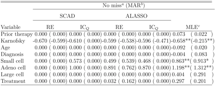
missing covariates using a sequence of one-dimensional conditional distributions as in Ibrahim, Lipsitz and Chen (1999), which we discuss in detail in Section 2.1. Our objective in the analysis of the LCCC 9719 dataset was to select the most important predictors of SCLC progression and estimate the parameters of the best model. These selection and estimation processes can be done simultaneously by combining one of the two penalty functions, SCAD or ALASSO, with one of the two penalty estimates, these being the random effects penalty estimate or the ICQ penalty estimate.
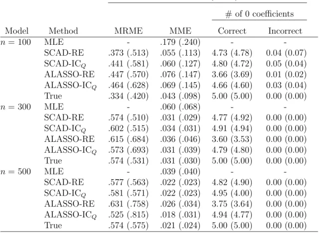
The rest of the paper is organized as follows. Section 2 gives the general development of maximizing the penalized likelihood function and estimating penalty parameters. In Section 3, we characterize the asymptotic properties of the MPL estimator and ICQ penalty selection procedures. Section 4 presents a simulation study which examines the finite sample performance of the MPL estimates and gives analyses of two lung cancer data sets. We conclude the paper with some discussion in Section 5.
3.2
Variable selection for the Cox model with
miss-ing covariates
3.2.1
Model formulation
the observed data and complete data respectively, for theith observation. Throughout this article, we assume that the covariates are MAR, i.e., the probability of a missing covariate does not depend on any of the observed covariate values (Little and Rubin, 2002). We also assume that the parameters of the missing data mechanism are distinct from the sampling model, so that the missing data mechanism need not be modeled in the complete data likelihood. We specify the joint distribution of (yi, δi,zi|xi) as a product of two conditional distributions,
f(yi, δi,zi|xi;θ) =f(yi, δi|zi,xi;θ)f(zi|xi;θ),
where θ includes all the unknown parameters. The generic label f(u1|u2) is used to denote the conditional distribution of u1 given u2. We assume that the parameters of the distribution of the censoring times are distinct from those of the distribution of the survival times and that the distribution of the censoring times is independent of the unobserved covariates. Under these assumptions, the conditional distribution of (yi, δi) given (zi,xi) can be written as
f(yi, δi|zi,xi;θ) = ft(yi|zi,xi;θ)δiSt(yi|zi,xi;θ)1−δifc(yi|xi)1−δiSc(yi|xi)δi, whereft, St, fc, and Sc are the density and survival functions of the survival time and censoring time, respectively.
We assume a proportional hazards model (Cox, 1975) for the failure times, which assumes that the hazard of subject i at failure time yi is λ(yi) exp((zTi ,xTi )β),where
as
f(yi, δi|zi,xi;β,Λ) ∝ λ(yi)δiexpδi(zTi ,xTi )βexp
n
−Λ(yi)e(z
T i,xTi)β
o
, (3.1)
where Λ(t) =Rt
0λ(u)du is the cumulative baseline hazard function. Note that we have ignored all terms that are independent of (β,Λ) and xi. Finally, following Ibrahim, Lipsitz and Chen (1999), we write the distribution of zi given xi as
f(zi|xi;α) =f(zi,q|zi,(q−1),· · · , zi,1,xi;α)× · · · ×f(zi,1|xi;α).
whereα are the parameters corresponding to the covariate distribution.
3.2.2
EM algorithm for maximizing the penalized likelihood
In the variable selection problem, our objective is to identify nonzero components ofβ
in (3.1) and simultaneously estimate all other parameters while accounting for missing covariates. We propose to maximize the penalized likelihood function, given by
`(θ)−n
p
X
j=1
φτj(|βj|) =
n
X
i=1
`i(θ)−n p
X
j=1
φτj(|βj|), (3.2)
where θ = (β,α,Λ), `i(θ) = log
R
f(yi, δi,zi|xi;θ)dzi,m is the observed-data log-likelihood for theith observation,τj is the penalty parameter corresponding to thej-th regression coefficient, and the penalty function,φτj(·), is a nonnegative, nondecreasing,
Because the observed-data log-likelihood function usually involves intractable inte-gration, we develop a Monte Carlo EM algorithm to compute the MPL estimator of
θ, denoted by θbτ, for each τ = (τ1, . . . , τp). Let Dc and Do denote the complete and
observed data for all subjects, respectively, and letLc(θ|Dc) = logf(Dc|θ) denote the complete-data log-likelihood function. At thes-th iteration, given θ(s), the E step is to evaluate the penalized Q-function
Qτ(θ|θ(s)) = Q(θ|θ(s))−n p
X
j=1
φτj(|βj|), (3.3)
where
Q(θ|θ(s)) = E{Lc(θ|Dc)|Do,θ(s)}=Q1(β,Λ|θ(s)) +Q2(α|θ(s)),
Q1(β,Λ|θ(s)) = n
X
i=1
Z
logf(yi, δi|zi,xi;β,Λ)f(zi,m|di,o;θ(s))dzi,m, and (3.4)
Q2(α|θ(s)) = n
X
i=1
Z
logf(zi|xi;α)f(zi,m|di,o;θ(s))dzi,m. (3.5)
Since the integrals in (3.4) and (3.5) are often intractable, we approximate these inte-grals by taking a Markov chain Monte Carlo (MCMC) sample of sizeLfrom the density
f(zi,m|di,o;θ(s)) (See Herring and Ibrahim, 2001). Let z (s,l) i = (z
(s,l)
i,m,zi,o), wherez (s,l) i,m is the l-th simulated value at the s-th iteration of the algorithm. The integrals in (3.4) and (3.5) can be approximated as
Q1(β,Λ|θ(s)) ≈ n
X
i=1
"
δilog{λ(yi)}+ 1
L
L
X
l=1
δi(z (s,l)T i ,x
T i )β
− 1 L
L
X
l=1
Λ(yi) exp
n
(z(s,l)Ti ,xTi)βo
#
,
Q2(τ|θ(s)) ≈ 1 L n X i=1 L X l=1
The M step involves maximizing Qτ(θ|θ(s)) with respect to (β,α,Λ). Rather than estimate the absolutely continuous function Λ(t), t ≥ 0, we estimate an increasing stepwise version of Λ. This involves maximizing with respect to (β,α) and the pa-rameters {Λ(xi) : δi = 1 for i= 1, . . . n}. Using this parametrization, the maximizers of Qτ(θ|θ(s)) are given by
β(s+1) = argmax
β
PQ1,τ(β|θ(s)),
α(s+1) = argmax
α
( n X
i=1
L−1
L
X
l=1
logf(z(s,l)i |xi;α)
)
,
λ(s+1)(yi) = δi
X
u∈R(xi)
1
L
L
X
l=1
exp(z(s,l)Tu ,xTu)β(s+1)
−1
,
Λ(s+1)(yi) = n
X
u=1
λ(yu)(s+1)1{yu ≤yi, δu = 1},
where
PQ1,τ(β|θ(s)) = PQ1(β|θ(s))−n
p
X
j=1
φτj(|βj|), and
PQ1(β|θ(s)) = n X i=1 1 L L X l=1
δi(z (s,l)T i ,x
T i )β−
n
X
i=1
δilog
X
u∈R(yi)
1
L
L
X
l=1
exp(z(s,l)Tu xTu)β
.
Maximizing Q2(α|θ(s)) with respect to α is straightforward and can be done using a standard optimization algorithm, such as the Newton-Raphson algorithm (Little and Schluchter, 1985; Schluchter and Jackson, 1989). Maximizing PQ1,τ(β|θ(s)) with re-spect to β, however, is very difficult since PQ1,τ(β|θ(s)) is a nondifferentiable and nonconcave function of β (Zou and Li, 2007).
expression for this approximation is given in the appendix document. Using this ap-proximation, PQ1,τ(β|θ(s)) resembles a penalized weighted least squares regression, so algorithms for minimizing penalized least squares can be used. Such algorithms include the local quadratic approximation algorithm (LQA) (Fan and Li, 2001) and the local linear approximation (LLA) algorithm (Zou and Li, 2008). We use the LLA algorithm because it reduces the computational cost of penalized maximizations (Zou and Li, 2008).
Using the approximation of PQ1(β|θ(s)), letβ(s+1)be the maximizer of PQ
1,τ(β|θ(s)). Since an approximation is used for PQ1(β|θ(s)),β(s+1) may not necessarily be the max-imizer ofQ1,τ(β|θ(s)). Following the ECM algorithm (Meng and Rubin, 1993), a value
θ(s+1) can be produced, such that Qτ(θ(s+1)|θ(s)) ≥ Qτ(θ(s)|θ(s)) rather than directly maximizing Qτ(θ|θ(s)). Therefore, we only need to obtain a β(s+1) which satisfies
Q1,τ(β(s+1)|θ(s)) ≥ Q1,τ(β(s)|θ(s)). This process is iterated until convergence and the value at convergence is denoted as θbτ. The value θbτ maximizes the penalized observed
data log likelihood function.
3.2.3
Penalty parameter selection procedure
To ensure thatθbτ has good properties, the penalty parameterτ has to be appropriately
selected. Two commonly used criteria for selection of the penalty parameter include the GCV and BIC criteria. These criteria cannot be easily computed in the presence of missing data, because they are functions of observed data quantities whose expressions require intractable integrals. Moreover, it has been shown in Wang et al. (2007) that even in the simple linear model, the GCV criterion can lead to significant overfit.
2009) selects the optimal τ by minimizing
ICQ(τ) = −2Q(θbτ|θb0) +cn(θbτ),
where θb0 = argmax
θ
`(θ) and cn(θ) is a function of the data and the fitted model. For instance, ifcn equals twice the total number of parameters, then we obtain an AIC-type criterion; alternatively, we obtain a BIC-type criterion when cn(θ) = dim(θ)×logn. Moreover, in the absence of missing data, ICQ(τ) reduces to the usual AIC or BIC criteria. As in the EM algorithm, we can draw a set of samples fromf(zi,m|di,o;θb0) for
i= 1, . . . , n in order to to estimateQ(θbτ|θb0) for any τ.
The random effects penalty estimator is calculated under the assumption that the regression coefficientsβ are distributed as random effects in a hierarchical model. The parameter τ can be regarded as a parameter in the distribution of β, denoted by
f(β|τ, n). Then, τ can be estimated by maximizing the marginal likelihood with respect to (α,Λ,τ), which is given by
Z n Y
i=1
Z
f(yi, δi,zi|xi;θ)f(β|τ, n)dzi,mdβ= n
Y
i=1
Z
f(di,o|θ)f(β|τ, n)dβ, (3.7)
wheref(β|τ, n) is defined by
f(β|τ, n) = p
Y
j=1
exp{−nφτj(|βj|)}/[C(τj, n)],
and C(τj, n) is the normalizing constant off(β|τj, n). The resulting estimate of τ, de-noted byτbRE, from the maximization of (3.12), is the random effects penalty estimator. Treating the regression coefficients as missing data, the EM algorithm can be used to calculate τbRE.