The Impact of Public Smoking Bans on Tobacco Consumption Behavior and
Environmental Tobacco Smoke Exposure in Argentina
By: Michael Catalano
Honors Thesis
Economics Department
The University of North Carolina at Chapel Hill
April 2016
Abstract
Acknowledgements
1
Introduction
Tobacco consumption represents the leading preventable cause of death and disease worldwide and one of the most significant global public health concerns, accounting for almost 6 million deaths annually (WHO, 2011). Due to strong international evidence of the serious short- and long-term health impacts of tobacco consumption, many developed nations have taken legislative action over the past few decades aimed to reduce consumption and reduce exposure of nonsmokers to environmental tobacco smoke (ETS). The mechanisms implemented include increased taxation, restrictions on advertising and distribution, the introduction of educational programs, and bans on smoking in public places. It is important to analyze the potential impact of each of these various policy changes on both short and long-term smoking behavior and health in order to determine the most effective methods of reducing consumption.
passed individual legislation that restricted public smoking to varying degrees, but it was not until 2011 that Argentina passed its first national tobacco control law, which extended a comprehensive public smoking ban to all 23 provinces (Georgetown Law, 2011).
effects of such bans on either consumption or secondhand smoke exposure, I incorporate and discuss the impact on both, for each has significant short and long-term health implications.1
My empirical analysis that controls for individual explanatory variables and time and province fixed effects predicts changes in consumption behavior that differ from what has been found in some previous economic studies. While many studies observe strong declines in both smoking prevalence and intensity among specific demographic groups after the implementation of bans, we see very slight reductions in consumption in Argentina, and even an increase for individuals with particular characteristics. Full and partial smoking bans appear to have no immediate effect on smoking prevalence among the general population, but a reduction in prevalence is associated with a full ban that has been in place for several years, indicating that it may take time for smoking behavior to respond or for the ban to be fully enforced. This effect is especially pronounced among young, wealthy males. The reduction in prevalence is associated with a decline in the number of individuals starting to smoke, rather than an increase in the number of individuals quitting smoking. In fact, there is some evidence that the bans may increase the cigarette consumption of current heavy smokers. A full provincial ban has no significant effect on the quantity of cigarettes smoked by individual smokers, and a partial provincial ban that allows smoking in designated areas is found to significantly increase smoking intensity among heavy smokers. These results imply that a full policy may reduce the number of individuals smoking, but a partial policy may be negatively affecting the behavior of heavy smokers. The effects on ETS exposure are more pronounced. Full public smoking bans are
1It is important to note that due to the unavailability of longitudinal survey data in Argentina, I am required to take an approach different than the majority of the previous literature on the effects of tobacco control policy—while many studies rely on panel data for such analyses, I analyze repeated cross-sectional data. Panel data are preferred in analyses of tobacco consumption due to the addictive nature of cigarettes and the dynamic decision- making
associated with a significant decline in non-smokers’ exposure to secondhand smoke, especially among the same demographic of young, wealthy males. My findings provide empirical evidence of the benefits associated with full public smoking bans and the potential harm caused by partial smoking bans, indicating that provincial policymakers should work to ratify and implement the full smoking bans outlined in the National Tobacco Control Law.
Section 2 of this thesis discusses the relevant literature in economics and public health on the impact of public smoking bans, both globally and within Argentina. Background of the recent history of tobacco legislation in Argentina is presented in Section 3. Section 4 provides a robust theoretical model of an individual’s smoking decisions and the factors that affect this decision, including the various forms of public smoking bans. After presenting the theoretical model, I introduce the repeated cross-sectional data source, describe dependent variables, and discuss the application of these data to theory in Section 5. I apply the concepts from theory and the available data to an empirical model and methodology, discussed in detail in Section 6. The results of the empirical analyses are presented and discussed in Section 7, and Section 8 concludes.
2
Literature Review
demand for cigarettes and to provide strong evidence that the passage of excise taxes could significantly reduce smoking levels. Later studies modified Lewit and Coate’s approach and analyzed how other factors affect the price elasticity of demand of cigarettes, and therefore the potential effectiveness of taxation. Wasserman et al. (1991) looked at price changes and demand shifts in the context of other tobacco control regulations and determined that other analyses may have overestimated the price elasticity of demand—their more robust analysis found a price elasticity of demand ranging from -0.02 in 1974 to -0.23 in 1985. Other studies have also incorporated the effects of addiction on demand. Becker et al. (1988) developed the first dynamic rational addiction model, a now widely referenced model that is based on the idea that past consumption is very strongly correlated with current consumption. Their model and empirical work indicate that addicts do not respond strongly to temporary and short-term price changes. Gilleskie and Strumpf (2005) expand upon this idea and find evidence that individuals with past cigarette consumption are likely to be less sensitive to cigarette price changes in the short-run than those that have never smoked. They conclude that price increases through taxation will have a greater aggregate effect in the long run than in the short run as individuals reduce consumption and move to the non-smoking, price-sensitive group.
group to a “control” group that does not face the treatment. When there is time and state variation in the implementation of tobacco control policies, difference-in-difference models allow the comparison of individuals within the states under legislation to those in the “control” states over time. Jones et al. (2015) used a series of difference-in-difference fixed effects models on panel data of tobacco consumption in the UK, and they found no significant change in smoking prevalence or cigarette consumption on an aggregate level after a public smoking ban was implemented, although significant changes were found amongst specific demographic groups. Anger et al. (2011) also used a difference-in-difference model to determine that public smoking bans did not have a significant effect on overall tobacco consumption in Germany; however, they significantly reduced consumption amongst those who frequent bars and pubs. Boes et al. (2015) conducted a similar analysis on smoking bans in Switzerland and concluded that they do significantly reduce smoking rates, but these reductions only begin to emerge one year after the ban. This study indicates the importance of accounting for time since the passage of the law.
Like Gilleskie and Strumpf (2005), Chaloupka et al. (1992) incorporated addictive behavior in cigarette consumption (i.e., the effects of tolerance, reinforcement, and withdrawal) in their analysis of the passage of public smoking bans in the United States. Using instrumental variable procedures to account for the endogeneity of past and future consumption, they found that the passage of basic public smoking bans significantly reduced average cigarette consumption among males in the United States, but it had no significant effect on women’s consumption.
cigarette prices on adult cigarette consumption in the United States uses cross-sectional data collected by the Centers for Disease Control and Prevention (CDC). While controlling for individual characteristics and state and time fixed effects, Taurus uses a two-part technique to separately model smoking prevalence and smoking intensity. The former is estimated with a probit specification, and the latter is estimated with a generalized linear model (GLM) with log-link and Gaussian distribution. The GLM is used because the smoking intensity variable is logarithmically transformed, and this method provides estimates interpretable on the original scale without having to manually retransform it. Smoking bans are characterized by a three-point scale representing varying strengths of enforcement. He finds a negative price elasticity of demand of -0.072, implying that taxation could significantly reduce consumption. However, his estimates predict that, although public smoking bans reduce average smoking intensity by up to 5.18 percent, they have very little impact on smoking prevalence.
exposure, but they may actually increase the exposure of nonsmokers to secondhand smoke by displacing smokers to private places. By analyzing cotinine levels to indicate exposure to cigarette smoke, they found that young children were actually more exposed to ETS after the implementation of the public smoking ban, a surprising and disheartening result.
Despite strong international interest, there has been limited economic analysis of tobacco consumption and control in Argentina. However, Konfino et al. (2014) published a public health analysis that predicted the long-term health impact of Argentina’s national tobacco control law. The prediction was based on available data from before the law, but it did not make use of data collected after the law’s passing. Rather, it relied on estimates from previous public health literature to predict changes in consumption levels. Like many other public health research papers, this type of analysis predicts a significant reduction in tobacco consumption and strong health benefits—it suggests a decline of 7500 coronary heart disease (CHD) related deaths by 2020, a reduction of about 3 percent per year. This estimated reduction is significantly greater than the results of previous economic studies in other nations, and my findings indicate that such significant health benefits are unlikely.
3
Public Smoking Bans
settings among public places or in specific rooms or open-air areas within venues. In order to account for policy implementation in this analysis, it is important to acknowledge the varying levels of restrictions and clearly differentiate between partial bans and full bans, for they affect both smokers and nonsmokers differently. For example, if smoking is prohibited in the main room of a bar or restaurant, but there is a designated room for smokers, it is much less likely that an individual will refrain from smoking than if there is no place to smoke, i.e. the loss of utility that an individual smoker attending that venue faces is expected to be lower than it would be if there was no place to smoke. There is also the potential for peer-effects that may influence smokers to smoke more by grouping them together and making the practice seem more socially acceptable. These concepts, as well as the decisions that smokers face in the presence of the bans, are expanded upon in the description of the theoretical model in Section 4.
The National Tobacco Control Law was passed in 2011 with the intention of imposing a comprehensive public smoking ban nationally; however, the implementation of the law did not actually require that all remaining provinces enact and enforce these bans. Rather, it was a strongly encouraged policy, but it was only required to be enforced if ratified by the individual provinces. The policy represents a strong change in national attitudes towards smoking, and it may have encouraged some bars and restaurants across the country to begin banning smoking. Yet, after its passage in 2011, only four provinces ratified it (and four additional provinces passed their own public smoking bans).2 A major reason for such a limited number of ratifying
provinces is the fact that many already had strong policies in place; however, seven provinces with regulations weaker than those imposed by the national law and five provinces that were
2 Two of the four provinces that ratified the national law actually had their own provincial smoking bans in place at
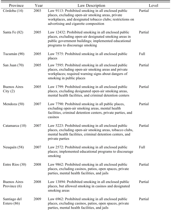
completely lacking regulations have yet to ratify the law. By 2013, between the subnational laws and the ratifications, 18 provinces and the capital city of Buenos Aires were covered by some level of smoking restrictions. The levels of public smoking restrictions and a description of exceptions to the law in various provinces are outlined in Appendix Table A1.
The series and progression of province-level smoking bans between 2004 and 2011 can be compared to those that were passed on city and state-levels in the United States beginning in 1980. Aspen, Colorado became the first city in the United States to require smoke-free restaurants in 1987, and San Luis Obispo, California became the first city in the world to ban smoking in all public buildings in 1990. Other cities and states followed this trend, and by 2012, 28 states and the District of Columbia had passed comprehensive smoke-free legislation (American Lung Association). A number of studies have been conducted on smoke-free legislation within the United States, which can serve as a useful and interesting comparison and potential check for external validity.
demographic statistics, and run a logistic regression on an indicator of the presence of a partial (or full) ban. I determine that there is no significant relationship between a province’s initial level of tobacco consumption in 2005 and its decision to implement either full or partial public smoking bans. The results of this regression are outlined in Appendix Table A2. This finding implies that the implementation of province-level policies was exogenous and can be thought of as randomly assigned; there is no need to worry about endogenous program placement.
4
Theoretical Framework
The theoretical model for this study captures the decision-making process of a smoker and the effect of public smoking bans on this decision-making process. Each period t, it is assumed that an individual receives utility from consuming cigarettes (Ct) and from consuming
other goods (Yt), with a utility function of u(Yt,Ct,St,Xt,εt). Because cigarettes are addictive
goods, it is important to take into account the effects of reinforcement, tolerance, and withdrawal; that is, the individual’s utility from smoking today depends on past smoking behavior up to the current period, or the addictive stock, St (Matsumoto, 2014). Exogenous
individual demographic and health characteristics (Xt), including age, gender, education,
household size, and BMI, may also impact the smoking decision. The error term εt represents
unobserved preferences or preference shifters that affect the utility of smoking.
utility from smoking in a social setting rather than at home or alone. In order to avoid modeling an individual’s decisions regarding location and time of smoking (because such detailed data are not available), the theory captures the disutility of a smoking ban generally by allowing the utility of smoking to depend on the type of smoking ban (i.e., full or partial). That is, the utility preference-ordering conditional on the type of ban is:
(1) where a full, comprehensive public smoking ban is represented by Btf, and a partial ban (meaning
that smoking is allowed in certain types of places or in designated smoking rooms) is represented by Btp.3
While bans impose these time and discomfort costs on smokers that result in lower indirect utility, it is possible that individual utility of smoking may be positively influenced or reinforced by designated smoking areas that increase the ratio of smokers to non-smokers. Peer effects have been most extensively explored in classroom settings between students but have recently become an area of inquiry in the field of health economics. For example, Fowler and Christakis (2008) explored peer effects and obesity using data from the Framingham Heart Study. They found that not only do obese individuals form social clusters, but an individual’s risk of becoming obese actually increases if he or she has a friend that becomes obese. Nakajima (2007) and Powell et al. (2005) investigated peer effects in youth smoking, and both studies found the existence of large and significant positive effects on smoking initiation. Based on this information, we assume that peer effects may play a role in smoking behavior in the presence of partial smoking bans—if smokers congregate in designated areas or rooms, they may actually
3 Note that this particular utility preference ordering represents a smoker; for a nonsmoker that frequents bars,
restaurants, and other public venues, exposure to secondhand smoke would likely present disutility, and the utility preference ordering would be the opposite of that shown here.
u(Yt,Ct,St,εt|Bt f
=1,Btp
=0)≤u(Yt,Ct,St,εt|Bt f
=0,Btp
=1)≤u(Yt,Ct,St,εt|Bt f
=0,Btp
smoke more than if they were in the main room of the bar with nonsmokers. In the designated areas their behavior may be more socially acceptable and reinforced.4
Each individual’s consumption is constrained by household income and the prices of cigarettes, PtC, and all composite goods, PtY, in the particular time period. An individual allocates
income to cigarettes, Ct, and all other goods, Yt:
(2) where the individual’s employment status is represented by Et, earned income is represented by It
if he or she works (i.e., Et=1), and non-earned income is denoted Nt.
The individual’s utility from smoking depends on his addictive stock, which evolves as follows:
(3)
where δt and γt represent the depreciation of current addictive stock and the effect of current
smoking levels on the next period’s addictive stock, respectively. As mentioned previously, addictive stock affects an individual’s utility through the effects of reinforcement, tolerance, and withdrawal. Reinforcement occurs when greater levels of past consumption of cigarettes and a corresponding increase in addictive stock cause the marginal utility of smoking and the desire for present consumption to increase. That is:
∂2u
∂S∂C>0
Simultaneously, the body becomes accustomed to increasing levels of consumption, and a physical process known as tolerance occurs, during which the individual must consume a greater
4
Based on this reasoning, positive peer effects will be minimal in the presence of full smoking bans.
Nt+ItEt =PtCC t+Pt
YY t
St+1=δtSt+γtCt
Vc(St,εt)=u(Yt,Ct =c,St,Xt,εt|Bt f
,Bt p
)+βE[max
c' Vc'(St+1,εt+1) |Ct=c] ∀t,c=0,1,...,C
quantity of cigarettes to achieve the same effect (i.e., greater levels of past consumption lowers current utility):
∂u
∂S<0
Finally, as the individual continues to consume cigarettes and his addictive stock grows, a physical dependence is generated. This dependence creates a withdrawal effect, through which the individual faces disutility when decreasing consumption:
∂u
∂C >0
This withdrawal effect makes it difficult for an individual to reduce consumption and ultimately quit smoking, and it explains why smokers are often insensitive to price increases and very rarely decrease consumption rapidly.
Based on these factors, an individual makes cigarette consumption decisions to maximize lifetime utility:
(4) where β represents a discount factor, and T is the end of life.
With an understanding of the evolution of the addictive stock, the individual’s budget constraint, and preferences including the implications of various levels of policy implementation on the utility an individual receives from smoking, the discounted present value of lifetime utility of each smoking level Ct =c in period t can be represented by the following recursive function:
(5) βtu(Yt
t=1
T
The error term εt is the alternative-specific error term capturing idiosyncratic utility of an
individual for each smoking alternative.5 The Bellman equation captures the lifetime value of a current smoking level Ct = c plus the discounted expected value of future optimal utility.6 The
discount factor is denoted β and characterizes how forward-looking an individual is in terms of smoking behavior (Gordon et al., 2015). This forward-thinking aspect is a vital component in the decision-making process, and it accounts for the effects of reinforcement and tolerance in cigarette addiction. Just as an increase in past consumption can increase the marginal utility of current consumption through reinforcement, an individual can also recognize that his level of current consumption will cause the marginal utility of future consumption to further increase. This may cause him to increase his current consumption. On the other hand, if an individual smokes heavily now and has a high level of addictive stock (i.e., a high level of tolerance), he may recognize that the utility he receives from the same level of consumption has declined and will continue to decline. This may cause him to restrict current consumption to increase future utility.7
The individual smoker’s problem is to select an optimal level of cigarette consumption today to maximize his expected lifetime utility. The derived demand for cigarettes is a function of the information available to an individual at the time of decision-making. That is:
P(Ct =c)=P(Vc(St,εt)>Vc'(St,εt)) ∀c'= f(St,Xt,Et,It,Nt,Pt C
,Pt Y
,Bt) (6) His behavior is influenced by the implementation of smoking bans in his province, among other things. His behavior also influences the utility and health of nonsmokers that spend time in
5 An example of a factor that could influence the error term ε
t is being unexpectedly diagnosed with bronchitis
today, which will cause the individual to receive lower utility from smoking in this period.
6 It is assumed that individuals believe whatever current smoking ban exists in their province today will exist in the
future. Changes in bans are surprises to individuals.
7 It is also important to note the effects of withdrawal here; an individual may wish to reduce his current levels of
proximity to the individual. The data and my empirical framework provide a means of quantifying and exploring the demand determinants and exposure consequences. Theory suggests that the implementation of public smoking bans will affect behavior by lowering the probability of consuming a particular quantity of cigarettes, c. That is:
∂P(Ct =c)
∂Bt
<0
As mentioned previously, bans impose time and discomfort costs on smokers that lower the utility of cigarette consumption. Furthermore, it is expected that the reduction in consumption associated with this disutility will increase over time after the passage of a ban. This effect is captured by the addictive stock, which is expected to decline each period with declining consumption, and it highlights the importance of exploring the effects of the bans over time.8
5
Data
5.1 National Risk Factor Survey
In order to empirically model the individual’s smoking decisions under various levels of policy implementation in Argentina, I utilize the National Risk Factor Survey (ENFR- Encuesta Nacional de los Factores de Riesgo), a stratified random survey distributed by Argentina’s National Ministry of Health in 2005, 2009, and 2013 (Ministerio de Salud). The ENFR project was initiated in 2005 due to a lack of national-level information on the risk factors for cardiovascular disease, a leading cause of death in Argentina. The survey is based on a questionnaire proposed by the Pan American Health Organization (PAHO) and the World Health Organization (WHO), and it has been received well by the Argentinian population with response
8 Recall that peer effects and reinforcement effects may alter this expected disutility in the presence of partial
rates of 87 and 75 percent in the first two survey distributions, respectively. By collecting these data, the Ministry of Health desires to develop effective new health policies and improve health promotion and preventative care strategies on a national level (Ferrante et al., 2007). The questionnaires and codebooks are available for each year, and the only variation in variables is due to the addition of new questions in later survey years.
The survey responses provide a number of variables that describe cigarette consumption behavior, including whether an individual has ever smoked, whether he or she currently smokes, how long he or she has smoked, how often he or she smokes, and how many cigarettes he or she smokes per day.9 They serve as dependent variables in my analysis, and they allow for conditional analyses to be conducted; that is, we can model both the extensive and intensive margins of smoking. I also include as a dependent variable in my analysis a binary variable that indicates whether an individual reports being regularly exposed to ETS in public places. This variable allows us to explore the impact of public smoking bans on both general exposure to ETS and nonsmokers’ exposure to ETS. Each survey wave contains health and demographic information, including age, gender, education, household size, employment, income, BMI, health insurance coverage, and self-reported general health level, on over 32,000 individuals aged 18 and over from general urban areas (cities with greater than 5000 inhabitants) in all 23 provinces and the capital city of Buenos Aires.
There are certain limitations of the data that must be acknowledged. One such limitation is that all data are self-reported, which presents the possibility of bias in some of the responses, such as underreported cigarette consumption. However, this is less of a concern due to the fact
that I focus on changes in consumption rather than absolute levels of consumption. It is also important to note that the data are repeated cross-sections rather than a panel of individuals, making it difficult to account for the addictive and dynamic nature of cigarette consumption and to follow specific individuals through different stages of policy implementation. Regardless of the non-panel nature of the data, prices of cigarettes vary over time but do not vary at the province level. As a result, an econometrician cannot include both the price of cigarettes and a time trend, as they would be perfectly collinear. There are also potential issues with variables that may restrict the precision of estimates. The income variable, for example, is reported as a range, and the midpoint of each range is used to construct a continuous measure of income. Also, due to the unavailability of accurate inflation data to calculate real income, I use deviations from the mean of nominal income each year.
Despite these limitations, the ENFR presents unique advantages. First of all, because it contains data on individuals from all provinces, I am able to include province indicators in my analysis in order to pick up non-time-varying, province-level unobservables that might influence cigarette consumption. Furthermore, it is the most extensive and reliable dataset on health characteristics and behavior in Argentina. The survey responses are thorough, and only 13 of 108,489 observations have been dropped due to missingness or incorrectly entered data. The ENFR provides the best data available to make reliable estimates on the impact of public smoking bans in Argentina.
5.2 Descriptive Analysis and Construction of Key Variables
Individuals surveyed in the ENFR are asked if they have smoked cigarettes at any point their lives. Approximately 52 percent of all individuals surveyed responded affirmatively to this question. All individuals are then asked if they currently smoke cigarettes. On average, 28 percent of individuals report currently smoking over the three survey years, and 54 percent of the individuals that report smoking in the past are still current smokers. A breakdown of the smoking status of Argentina’s population, by year, is presented in Figure 1.
Figure 1: National smoking prevalence, by year
Note: We see a greater rise in the proportion of individuals that have never smoked, compared to the number of individuals that are former smokers, as the proportion of current smokers declines. Part of this unbalance is likely due to the cross-sectional nature of the data and the entrance of new individuals in the sample, but this could also represent the fact that older smokers are passing away and younger individuals are not beginning to smoke at the same rate.
Figure 2: Daily smoking quantity, occasional smokers and heavy smokers
Note: The distributions indicate that individual responses to the number of cigarettes smoked per day are clustered at intervals of 5, and more strongly at intervals of 10.
29.91% 46.51% 23.58% 27.65% 47.41% 24.94% 25.7% 49.1% 25.2% 2005 2009 2013 Current Smokers Never Smokers Former Smokers
Graphs by Survey Year
Smokers, Former Smokers, & Never Smokers, by Year
Smoking Status of Argentina's Population
0 1000 2000 3000 4000 F re q u e n cy
0 10 20 30 40 50
Cigarettes smoked per day Occasional Smokers Smoking Quantity 0 1000 2000 3000 4000 5000 F re q u e n cy
0 10 20 30 40 50
Figure 3: Daily smoking quantity, by gender and age
Finally, all individuals are asked a series of questions regarding ETS exposure, including whether or not they are regularly exposed to ETS in public places. Younger individuals tend to report the highest levels of ETS exposure, for they likely spend the most time in restaurants, bars, and other venues at which smoking is most prevalent. Approximately 46.9% of the overall population reports being regularly exposed to ETS; however, only 38.2% of nonsmokers report regular ETS exposure. This difference is presented graphically in Figure 4, and it implies that smokers spend more time around other smokers than nonsmokers do.
Figure 4: ETS Exposure, by age and smoking status
0 10 20 30 40 50
18-24 25-34 35-49 50-64 65+
All smokers, by gender & age Smoking Quantity Males Females 20 40 60 80 A ve ra g e Pe rce n ta g e o f In d ivi d u a ls Exp o se d t o ET S
18-24 25-34 35-49 50-64 65+
Age Range
Smokers Non-Smokers
By Age & Smoking Status
The summary statistics of the main demographic and health variables for the overall sample, current smokers, and current nonsmokers are displayed in Table 2. The average age of the sample is 44.3, males make up 43.5 percent of the surveyed individuals, about 4.4 percent of surveyed individuals are unemployed, and average monthly income is about AR$1823.10 There are some noticeable differences between the average characteristics of smokers and nonsmokers. Smokers tend to be younger—the average age of smokers in the sample is 39.5, while the average age of nonsmokers is 46.2. Males are also significantly more likely to smoke than females, and smokers are less likely to have completed university-level education. These variables are used in my empirical analysis to control for individual variation that might explain observed smoking behavior.
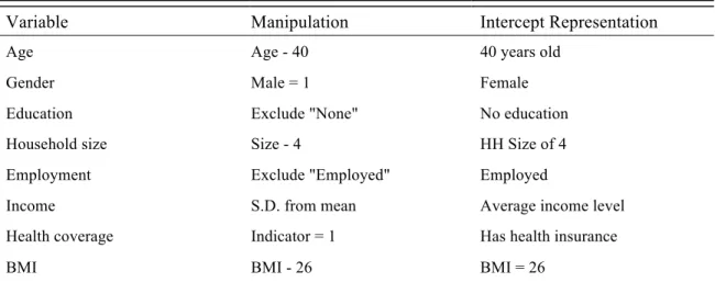
The independent variables are normalized in such a way that the constant term in each regression represents the expected smoking behavior of an individual with a particular set of characteristics: a 40 year-old female living in a household with four people in the province of Buenos Aires in 2005; she has completed secondary education, is employed, has the mean national income for each year (AR$858 in 2005, AR$2255 in 2009, and AR$2536 in 2013), has health insurance, and has a BMI of 26. The variable manipulation and my “normalized” individual are outlined in Appendix Table A3.
6
Empirical Framework
6.1 General Methodology
The solution to the individual’s optimization problem yields a demand function for smoking that depends on the arguments of the value function defined in Section 4. Specifically, we summarize the demand function for the number of cigarettes smoked per day and its arguments as:
(7) where Ct indicates the number of cigarettes consumed. Cigarette consumption is skewed right
with a corner solution at zero (Ct = 0), and a large proportion of the sample reports this zero level
of consumption (Figure A1, Appendix A). These individuals are, intuitively, nonsmokers. We desire to understand how these variables explain the probability of any use of cigarettes (i.e., P(Ct > 0)), as well as the level of current smoking conditional on having some level of
consumption (i.e., Ct | Ct > 0).
Exogenous demographic variables Xt described in Section 5 are included as controls in
the empirical analysis. Individual income It and non-earned income Nt are accounted for jointly
in the data, for the reported income represents overall household monthly income. Fixed province effects are contained in σp to account for variation in smoking prevalence and
consumption behavior between provinces, and time variation is controlled for through time fixed effects, σt. As mentioned previously, due to the lack of province-level variation in cigarette
prices and the three cross-sectional data points, price data PtC is perfectly collinear with time
fixed effects indicators. These indicators therefore pick up the effects of price changes, along with numerous other factors that influence changes in consumption over time. Finally, indicators for the presence of both partial and full smoking bans and variables that quantify the number of
Ct = f(St,Xt,Et,It,Nt,PtC,B
years since full or partial ban implementation are contained in Bt. The coefficients on these
variables allows for estimation of the immediate effects of the policy implementation and the effects of that policy over time.11
Theory suggests that one’s history of smoking, or the addictive stock St, impacts current
smoking behavior. Unfortunately, our data are cross sectional and do not include information on dynamic changes in smoking behavior. However, the data do include information on whether an individual has ever smoked in the past. We use this variable to separate current nonsmokers into never smokers or former smokers. When estimating whether or not an individual currently consumes any level of cigarettes, we can use the full sample or restrict it to those individuals who have smoked at some point in the past. We also know the age at which an individual began smoking, and we control for the age of initiation when explaining the level of consumption conditional on being a current smoker. Among current smokers of the same age, those who began smoking at a younger age are likely to have more years of smoking experience (i.e., a larger addictive stock).
The survey also asks individuals to report if they are occasional or heavy smokers. We define the regularity of smoking by the indicator Rt and assume that the same vector of
determinants explain regularity of smoking. That is:
P(Rt = j)= f(St,Xt,Et,It,Nt,Pt C
,Bt,σt,σp,εt), j=0,1, 2 (8) where regularity of smoking is never (j=0), occasionally (j=1), and everyday (j=2).
The bans were implemented in the hopes of minimizing secondhand smoke exposure in public places. I estimate the effects of the smoking bans on ETS exposure, as reported by individuals in the full sample. Exposure to ETS is modeled as:
P(Ot=1)= f(Xt,Et,It,Nt,Pt C
,Bt,σt,σp,εt) (9)
where Ot is a binary variable that indicates whether an individual is regularly exposed to
secondhand smoke in public places and serves as the dependent variable. I assume exposure depends on similar inputs of demographic characteristics, employment, income, cigarette prices, and policy implementation act as independent variables. Addictive stock is not included as an input. Obviously, individuals who smoke will experience more ETS as they are more likely to associate with others who smoke. I estimate the effect of public smoking bans on second-hand smoke exposure using the full sample (i.e., the general population) and nonsmokers specifically.
6.2 Conditional Regressions
There are two potential methods to account for endogenous selection in regression analysis—a multiple-part model based on conditional regressions, and a Heckman selection model. The Heckman selection model presents the opportunity to estimate potential smoking levels among the entire population rather than focusing only on smokers. However, the multiple-part model is used more often than the Heckman selection model when studying tobacco consumption for two primary reasons: researchers often want to quantify and predict actual smoking levels rather than potential smoking levels, and it is often difficult to find an exogenous factor that influences whether or not an individual is a smoker but does not affect the quantity that he or she smokes. Madden (2006) compared the results and the significance of these two models to describe tobacco consumption, and he found a two-part model to be stronger for both theoretical and statistical reasons. For the aforementioned reasons, I use a multiple-part model. Furthermore, I test a Heckman selection model without an exclusive restriction to model the probability of ever smoking jointly with the probability of currently smoking. Although the standard errors are inconsistent, I find the correlation coefficient, which measures the correlation between the errors of the two equations, to not be significantly different than zero. A similar strategy for current smoking participation and the level of smoking conditional on any smoking is used, and it does not converge.
alternative model could be used to explicitly model the correlation between the error terms, as done by Gilleskie and Strumpf (2005); this represents an avenue for further study.
6.3 Functional Form and Model Selection
My analysis begins by examining the effects of public smoking bans on smoking prevalence, using the binary current participation variable that indicates whether or not an individual smokes. Smoking prevalence is important to policymakers in Argentina because of the health implications associated with smoking. Numerous studies have found large and significant differences in both disease risk and life expectancy between smokers and nonsmokers. I measure determinants of smoking prevalence among both the general population and those individual with any smoking history prior to the survey. The regressions that are estimated using a standard logit model take the following form (in log odds):12
log[P(Ct>0)
P(Ct=0)
]=α0+a1Xt+a2Et+a3It+a4Nt+a5Pt C
+δBt+σt+σp+εt
(10)
log[P(Ct >0 |St>0) P(Ct =0 |St>0)
]=α0+a1Xt+a2Et+a3It+a4Nt+a5Pt C
+δBt+σt+σp+εt
where the first represents the probability of smoking any quantity of cigarettes in period t, and the second represents the probability of smoking any quantity of cigarettes in period t conditional on having smoked at some point in the past. I use a positive addictive stock variable to differentiate individuals with any smoking history from those who have never smoked a cigarette.
12 Note that Greek letters α, δ, σ, and ε differ across equations, but they are kept similar in the depiction of my
After determining the effects of smoking bans on the proportion of the population that smokes, I look more specifically at smoking intensity, or the level of smoking. I begin with an analysis of the regularity of smoking. I use a multinomial logit approach with a base outcome of not smoking at all (Rt = 0), and two alternate outcomes of smoking occasionally (Rt = 1) and
smoking heavily (Rt = 2). The coefficients estimated for these two outcomes represent the
relative likelihood that an individual is that “type” of smoker compared to the likelihood that the individual is a nonsmoker. The regressions take the following functional form:
log[P(Rt= j) P(Rt =0)
]=α0+a1Xt+a2Et+a3It+a4Nt+a5Pt C
+δBt+σt+σp+εt, j=1, 2
(11)
log[P(Rt= j|St >0)
P(Rt =0 |St>0)
]=α0+a1Xt+a2Et+a3It+a4Nt+a5Pt C
+δBt+σt+σp+εt, j=1, 2
As done with smoking prevalence, these equations are estimated using the general population and those individuals with a smoking history. The multinomial logit estimator allows for different marginal effects of explanatory variables on each regularity outcome.
In addition to observing participation and regularity, I observe the smoking intensity of individuals who choose to smoke currently. Health outcomes are known to differ across non-smokers and non-smokers, as well as among those who smoke at different levels, so the findings of this analysis have important health implications.13 For that reason, after evaluating the effect of the smoking bans on the proportion of the population that smokes and the proportions that smoke occasionally and heavily, I investigate the effect of the ban on smoking intensity among smokers. Due to the differences in behavior and addictive stock between those that smoke occasionally
and those that smoke everyday, I also estimate the effects of the policy on smoking intensity for occasional smokers and heavy smokers separately, as these individuals may react differently to the smoking bans. These regressions take the following form:
Ct|Ct>0=α0+a1Xt+a2Et+a3It+a4Nt+a5Pt C
+δBt+σt+σp+εt (12)
Ct|Rt =1=α0+a1Xt+a2Et+a3It+a4Nt+a5Pt C
+δBt+σt+σp+εt
Ct|Rt=2=α0+a1Xt+a2Et+a3It+a4Nt+a5Pt C
+δBt+σt+σp+εt
As mentioned previously, the number of cigarettes smoked per day is technically reported as a count variable, but it can be modeled as a continuous variable as well. In order to complete a robust analysis of the effects of smoking bans on smoking intensity, the variable is analyzed in both forms. I use an ordinary least squares (OLS) approach to model the smoking intensity variable, as well as its natural log, as continuous variables. I also conduct a quantile regression of the smoking intensity variable for all smokers to determine whether the public smoking bans have had different effects at different levels of smoking intensity. To explore the sensitivity of the estimated marginal effects of the ban to distributional assumptions, I also use a generalized linear model (GLM) with a gamma distribution. A gamma distribution is selected over a negative binomial distribution and Poisson distribution due to the nature of the data and the fit of each distribution. Figure A2 of the Appendix presents a visualization of each of these three distributions fitted using the actual smoking intensity data (conditional on being a current smoker) and plotted against it, and it is clear that the gamma distribution fits most closely.
presents significant and often underestimated health risks.14 While my previous analyses focus on modeling individual determinants of one’s own smoking behavior, this analysis investigates individual responses directly affected by the smoking behavior of other individuals. The binary dependent variable that indicates whether an individual reports being regularly exposed to ETS in public places (Ot) is analyzed using a standard logit model with the following form:
log[P(Ot=1)
P(Ot =0)]=α0+α1Xt+α2Et+α3It+α4Nt+α5Pt C
+δBt+σt+σp+εt (13)
log[P(Ot=1 |Ct=0) P(Ot =0 |Ct =0)
]=α0+a1Xt+a2Et+a3It+a4Nt+a5Pt C
+δBt+σt+σp+εt
Where the first captures the effects of determinants on exposure response of all individuals regardless of own smoking behavior, and the second captures the marginal effects on exposure to those individuals who do not currently smoke.
7
Results
7.1 Smoking Prevalence
The results from logit regressions that explain the current smoking probability are provided in Table 3. The effects of ban implementation, demographic characteristics, employment, and income are presented as log-odds ratios. I estimate the probability of current smoking using the full sample unconditional on one’s history of smoking, and for those individuals who report having ever smoked (St > 0).15 In order to investigate heterogeneous
effects of the smoking ban, I estimate the model without interactions (Specification 1) and with
14 A study conducted by Barnoya and Glantz (2005) found that the cardiovascular health risks presented by ETS
exposure are, on average, 80% to 90% as large as those from active smoking.
15 Note that for all individuals, the regressions estimate the probability of being a smoker versus a nonsmoker; for
interactions (Specification 2). Marginal effects are presented in Appendix Table A4 to aide in interpretation of results.16
The implementation of a full or partial ban does not significantly impact average smoking prevalence in Argentina in the first year that it is implemented. However, there is a significant effect at the 10% level of the full ban that reduces smoking each year after the first year of implementation (Specification 1). This finding implies that, although the implementation of a full ban does not have an immediate effect on smoking prevalence, there is a reduction in prevalence over time. The marginal effects simulations predict an overall reduction in smoking prevalence of about 1.0 percent one year after the implementation of a full ban and 2.2 percent five years after the implementation of a full ban. Specification 2 suggests that younger individuals and individuals with higher income are impacted by a full ban.17
Partial bans do not have any significant effect on prevalence among the general population, but males are less likely to smoke if a partial ban is in place, as are individuals with higher income. As individuals age, however, partial bans appear to encourage smoking. This latter finding suggests the importance of differentiating the effects of the bans on smoking initiation and continuation, since initiation of smoking at older ages is rare and addiction to smoking is more likely at older ages.
Recognizing that there are individuals who have never smoked and who may be indifferent to the ban, I estimate the impact of the bans on those individuals with some history of smoking. Table 3 indicates that, in general, the bans have no immediate or long-term effect on
16 Marginal effects for all regressions were simulated manually in order to properly capture the effects of different
functional forms and interactions between variables.
17 The interactions of gender, age, and income with the implementation of partial bans are significant, and the signs
current smoking probabilities of individuals that have ever smoked (Specification 1). However, the partial ban reduces the probability of smoking among males and both the full and partial ban deter smoking as income rises.
While the public smoking ban variables provide the greatest insight into the effects tobacco control policies over time, the time indicator variables also have important implications. For all four regressions presented in Table 3, the coefficients on the indicators for the year 2009 and the year 2013 are negative and significant, and the value of the coefficient on the 2013 indicator is significantly greater than the 2009 indicator. Generally, the negative coefficients on these variables imply that unobserved aggregate factors influence smoking prevalence of all individuals over time. Because the data on smoking prevalence is observed only three times, however, I cannot confirm the functional form of the aggregate impact. The larger coefficient on the 2013 indicator variable, however, indicates that there may have been a cultural shift or a change in national attitudes towards smoking after the passage of the National Tobacco Control Act of 2011 that contributed to a reduction in prevalence. So, while not all of the provinces ratified and enforced the national legislation, there may have been venues and cities that independently took action and implemented bans. It is possible that the 2013 indicator accounts for some indirect effects of the legislation.
a lower propensity to smoke as household size increases and body mass increases. Interestingly, those individuals with health insurance, all else equal, are more likely to smoke. This finding may suggest selection into health insurance by individuals more likely to need it (i.e., adverse selection) or an increased likelihood to engage in poor health behaviors as a result of being insured (i.e., ex ante moral hazard).
Marginal effects simulations reveal that the probability of smoking decreases for an individual by 0.2 percentage points per year past the age of 40 (and increases by 0.2 percentage points per year for each year under the age of 40), males are 9.0 percentage points more likely to smoke than females, those with university education are 6.0 percent less likely to smoke than those with secondary education, and employed individuals are 2.8 percentage points less likely to smoke than unemployed individuals. Income is significant at the p<0.10 level, and for each standard deviation above the mean income, an individual is 0.3 percentage points less likely to smoke. An individual is 0.6 percentage points less likely to smoke for each additional household member. Finally, an individual is 4.4 percentage points more likely to smoke if he has health insurance, and the probability of smoking increases by 1.0 percentage point for each two-point increase in BMI.
7.2 Smoking Frequency
determine if this decline is due to a reduction in the number of people smoking occasionally or heavily. A multinomial logit model, the results of which are presented in Table 4, is estimated to answer this question. The model is again estimated using the full sample unconditional on one’s history of smoking and for those individuals who report having ever smoked (St > 0), and the
outcomes of being an occasional smoker and a heavy smoker are analyzed against the base case of being a nonsmoker. Marginal effects estimates for each outcome are presented in Appendix Table A5.
Similar to the results of the logit models for smoking prevalence, we do not see any reduction in heavy or occasional smoking behavior in relation to the passage of public smoking bans among those with any smoking history. This provides further support to show that the ban has not significantly influenced individuals to quit smoking. However, among all individuals in the sample, although there is no immediate impact of the ban, there is an estimated reduction in heavy smoking behavior several years after the implementation of a full smoking ban, and this estimate is significant at the p<0.10 level. It is estimated that there is a reduction in the proportion of heavy smokers among the entire population by 0.6 percentage points one year after the implementation of a full ban in a particular province, and 1.4 percentage points five years after the implementation of a full ban. Although the estimates are not significant for the occasional smoking outcome, the marginal effects simulation predicts a reduction in occasional smoking behavior by 0.7 percentage points five years after the implementation of a full ban. These five-year reductions ultimately correspond with an increase in the proportion of nonsmokers by 2.0 percentage points.18 The results also suggest that younger individuals and
18 This estimate aligns closely with the predicted reduction in smoking prevalence of 2.3 percentage points predicted
individuals with higher levels of income are affected more by the passage of a full ban,
particularly in the reduction of heavy smoking behavior.
While the results presented in Table 4 indicate that a full ban is associated with a
reduction in heavy smoking prevalence among the entire sample, they also suggest an increase in
the probability of being a heavy smoker a number of years after the passage of a partial ban.
There is an estimated increase in the probability of being a heavy smoker by 1.4 percentage
points five years after the implementation of a partial ban. Although the coefficients are not
significant, partial bans are also estimated to be associated with a 0.1 percentage point decline in
the proportion of the population that smokes occasionally and a 1.3 percentage point decline in
the proportion of nonsmokers five years after the implementation of a partial ban. As discussed
in the theoretical framework in Section 4, this effect can likely be partially attributed to peer
effects that arise when smokers are congregated in specific smoking rooms and the practice of
smoking becomes more socially acceptable and is reinforced. Estimates for interaction terms
indicate that the observed increase in heavy smoking is even greater among females, older
individuals, and less wealthy individuals.
Just as seen with the logit model for smoking prevalence, the coefficients on the year
indicator variables for the outcomes of occasional and heavy smoking are negative and
significant, further reinforcing that there has been a downward trend over time in smoking
behavior. However, the magnitude of the coefficient on the 2013 indicator is only significantly
greater than the coefficient estimate for the 2009 indicator for heavy smoking behavior, not for
occasional smoking behavior. This implies that the indirect effects of the National Tobacco
than reducing occasional smoking. This estimate provides evidence in support of the model’s
prediction that full bans reduce the proportion of heavy smokers in the population.
The multinomial logit model also estimates that, among all individuals in the sample, the
prevalence of occasional smoking declines by about 0.2 percentage for every year of age past the
age of 40 while the prevalence of heavy smoking is not strongly correlated with age. Males are
2.6 percentage points more likely to be occasional smokers and 6.6 percentage points more likely
to be heavy smokers than females. Those with university education are predicted to be 1.1
percentage points less likely to be occasional smokers and 4.9 percentage points less likely to be
heavy smokers than those with secondary education, and employed individuals are 1.4
percentage points less likely to be occasional smokers and 1.3 percentage points less likely to be
heavy smokers than unemployed individuals. Individuals with health insurance are more likely to
smoke both occasionally and heavily relative to not smoking, and individuals with higher BMI
levels are less likely to be heavy smokers. Finally, individuals with larger households are less
likely to smoke both heavily and occasionally. While Section 7.1 explored the effects of these
characteristics on smoking prevalence, these estimates provide a breakdown of how regularly
various smokers of different demographic backgrounds are smoking.
7.3 Smoking Intensity
Now that I have presented the effects of public smoking bans on smoking prevalence and
frequency in Argentina, I focus on the individuals that do smoke in order to determine the effects
of the policy on smoking intensity. I estimate the expected levels of smoking intensity for all
reports, on average, how many cigarettes an individual smokes per day. By conditioning the
regressions on only current smokers, I eliminate all zeros from the data for this variable. As
mentioned in Section 6, I complete this analysis using three different models—a general ordinary
least squares model (OLS) on both the reported smoking intensity variable and the natural log of
the smoking intensity variable, a quantile regression that allows us to determine the effect of the
bans on smokers at different levels of smoking intensity, and a generalized linear model with a
gamma distribution in order to model the variable as non-continuous and capture non-linear
effects. The results of these regressions are presented in Table 5, Table 6, and Table 7,
respectively, and the marginal effects estimates for the OLS and GLM are presented in Appendix
Table A6.
While I find that full smoking bans are associated with a decline in smoking prevalence, I
observe a lack of a significant association between full bans and smoking intensity. An even
more troubling result presented by these three models is the significant increase in smoking
intensity among heavy smokers, and, more specifically, the heavy smokers who smoke at an
intensity in the top quartile of all smokers, after the implementation of a partial policy. The OLS
regression predicts that, among all smokers, the implementation of a partial smoking ban is
associated with a significant increase in smoking intensity of approximately 0.797 cigarettes per
day. The OLS regression on the natural log of smoking intensity and the GLM also predict
positive and significant coefficients that correspond to similar marginal effects.19 It is estimated
that five years after the implementation of a partial smoking ban, smoking intensity increases by
approximately 0.897 cigarettes per day among all smokers.20 The variable that indicates the
number of years since the passage of a partial ban is also positive, but it is not significant, indicating that these types of policies actually have strong immediate effects on consumption rather than effects that accumulate and grow over time.
It is also important to analyze the estimates of these same models while conditioning on both occasional smoking behavior and heavy smoking behavior in order to gain a more robust understanding of how these policies affect different types of smokers. Occasional smokers are often younger individuals that only smoke in social settings with friends, so it would be expected for public smoking bans to affect the smoking intensity of these individuals most strongly. This, however, is not the case, and we do not see any significant effect of either a full or partial smoking ban on smoking intensity among occasional smokers. The reason that we observe a significant increase in smoking intensity among the entire population of smokers after the implementation of a partial ban is the fact that heavy smokers significantly increase their consumption in the presence of such bans, and this increase drives up the entire population statistic. The OLS model predicts an average increase of 0.941 cigarettes smoked per day by heavy smokers after the implementation of a partial ban. This corresponds to an estimated increase in intensity of 1.086 cigarettes per day five years after the implementation of the ban.21 Although the utility preference-ordering conditional on the type of smoking ban in my theoretical framework (Section 4) predicts that a partial ban would lower the utility of smoking for an individual relative to the lack of a ban, it is important to consider the influence that peer
20 The OLS of the natural log of smoking intensity predicts an increase in cigarette consumption by 6.8% per day,
and the GLM predicts an increase of 0.850 cigarettes per day.
21 The significant coefficient in the OLS regression of the natural log of smoking intensity predicts an increase in
effects have on smoking behavior and the possibility that they might actually influence consumption levels to increase.22 A partial ban establishes peer effects by having smokers gather in designated spaces, and we see that this strategy has had counteractive effects on heavy smoking behavior.
Beyond determining that smokers that smoke every day are the individuals that are increasing their smoking intensity under partial public smoking bans, I also determine that the individuals that smoke the highest quantities of cigarettes are impacted even more strongly by these partial bans. Table 6, which presents the results of a quantile regression at each quartile, indicates that while the effect of partial bans (and full bans) is not significant for individual smokers at the first and second quartiles of smoking intensity, it has a positive and significant coefficient for individuals at the third quartile, which corresponds to a smoking intensity of about 16 cigarettes per day. The model predicts that a partial ban is associated with an increase in consumption among smokers at this level of smoking intensity by about 0.890 cigarettes per day. This indicates that the increase in consumption associated with the partial smoking ban is greatest among those that smoke everyday at the highest intensity.
Another interesting difference between changes in smoking prevalence and smoking intensity is that smoking intensity has not steadily declined over time as prevalence has (i.e., the proportion of individuals that smoke has steadily declined over time, but those that do smoke are not smoking any less per day). This is determined based on the lack of a significant relationship between the year indicator variables and smoking intensity in any of the three models used; while we saw a significant negative coefficient on both year indicator variables for smoking
22 If heavy smokers spend more time with other heavy smokers at bars, they will likely be more inclined to smoke a
prevalence and regularity, neither coefficient is significant at the p<0.10 level here. This is a very important finding that has significant implications for smoking behavior in Argentina. As stated previously, there were unobserved aggregate factors over time and a general cultural shift in relation to the passage of the National Tobacco Control Law of 2011 that contributed to a reduction in prevalence, but these factors did not have the same effect on smoking intensity. This implies that those same factors either did not influence smoking intensity, or that they were offset by some other change over time that affected intensity while having a minimal effect on prevalence. One such change that could have contributed to this is the increase in affordability of cigarettes over time. The price of cigarettes is not included in these models due to a lack of province-level variation and a corresponding perfect multicollinearity with the time indicator variables, and, due to inaccurate inflation data reporting since 2007 in Argentina, it is often difficult to estimate the real price of different goods. However, using quarterly household income data from Argentina’s Personal Household Survey (EPH- Encuesta Permanente de Hogares) and monthly cigarette price data from the Ministry of Agriculture, I am able to determine the number of packs of cigarettes that can be purchased at the average monthly income for each quarter, a relative measure of the affordability of cigarettes.23 This information is presented in Figure 5,
and it is clear that cigarettes have steadily become more affordable to the general population over time. Prices and affordability are more likely to affect the number of cigarettes smoked than the decision of whether to begin smoking, so it is possible that this increase in affordability has worked against the general downward trend in smoking behavior over time. This presents an exciting opportunity for future studies, and, potentially, important implications for policymakers
23 The EPH is a survey that has been distributed quarterly since 2003. It is a rotating panel dataset that contains