A new model for integrated lot sizing and scheduling in flexible job
shop problem
Mahmoud Fadavi1, Rashed Sahraeian1*, Mohammad Rohaninejad1
1
Industrial Engineering Department, College of Engineering, Shahed University, Tehran, Iran [email protected], [email protected], [email protected]
Abstract
In this paper an integrated lot-sizing and scheduling problem in a flexible job shop environment with machine-capacity-constraint is studied. The main objective is to minimize the total cost which includes the inventory costs, production costs and the costs of machine’s idle times. First, a new mixed integer programming model, with small bucket time approach, based on Proportional Lot sizing and Scheduling Problems (PLSP), is proposed to formulate the problem. Since the problem under study is NP-hard, a modified harmony search algorithm, with a new built-in local search heuristic is proposed as solution technique. In this algorithm, it is improvised a New Harmony vector in two phases to enhance search ability. Additionally, Taguchi method is used to calibrate the parameters of the modified Harmony Search (HS) algorithm. Finally, comparative results demonstrate the effectiveness of the modified harmony search algorithm in solving the problem.It is also demonstrated that the proposed algorithm can find good quality solutions for all size problems. The objective values obtained by proposed algorithm are better from HS algorithm and exact method results. Keywords: Lot-sizing, scheduling, flexible job shop, Harmony Search algorithm (HS)
1- Introduction
The Flexible Job Shop scheduling Problem (FJSP) is a generalization of the classical Job Shop Problem (JSP). In JSP, n jobs are processedon m unrelated machines, and the route each job takes on different machines is known. Moreover, processing times are fixed and all the machines are assumed to be available at time zero. FJSPextends JSP by assuming that, there is at least one instance of the machine type necessary to perform each given operation (Fattahi et al., 2009). In other words, the main difference between JSP and FJSP is that the latter should choose a machine from a set of candidate machines to perform an operation. The FJSP is strongly NP-hard even with two machines where each job has at most three operations (Fattahi et al., 2007). In turn, the problem under study which is a combination of FJSP and integrated lot sizing would be strongly NP-hard (Karimi et al.,2003).
Generally, production problems can be classified into three categories based on the time intervals; long term, medium term, and short term. Production planning is included in the medium-term level and scheduling is placed in the short-term level. Integrated production planning and scheduling problem,
*Corresponding author.
ISSN: 1735-8272, Copyright c 2017 JISE. All rights reserved Journal of Industrial and Systems Engineering
Vol. 10, No. 3, pp 72-91 Summer (July) 2017
73
are quite important in the production planning. In order to find the optimal solutions, interrelationship between these two levelsshould be considered, and the planning decisions should be taken simultaneously (Ramezanian & Saidi-Mehrabad, 2013). In recent years, to meet the need for more precise and realistic production planning, many papers have been publishedabout simultaneous optimization of lot-sizing and scheduling (Rohaninejad et al., 2015b).
Due to the NP-hardness of the problem under study, heuristic methods are used. In comparison with exact methods, these approaches are more reasonable in regard to the computational times. In recent years, the use of meta-heuristics such as Tabu Search (TS) and Genetic Algorithms (GAs) has led to better results than classical dispatching or greedy heuristic algorithms. Similarly, in the current study, a harmony search algorithm (HA) is modified and developed to solve the model.
In the following section, a brief review on integrated lot sizing and scheduling problems are given. In section 3, the mixed integer programmingformulation of the problem is presented. In section 4, the proposed solution techniques are presented. Computational results of solving the model, both with IBM ILOG CPLEX software andthe proposed algorithm are reported in Section 5. Section 6 concludes the paper and discussesits possible extensions.
2- Literature Review
Small bucket time models and big bucket timemodels are two basic modeling approaches for simultaneous optimization oflot-sizing and schedulingproblems.In the small bucket time models, one or at most two items may be producedin everyperiod. Three common types of models in small bucket time models are discrete lot-sizingscheduling problem (DLSP), continuous setup lot-sizing problem (CSLP) and proportionallot-sizing scheduling problem (PLSP). The PLSP model was first introduced by Drexl and Haase (1995). In PLSP model, the micro period is increased by increments in the computational complexity of the model (Rohaninejad et al., 2015c). Integrated lot-sizing and scheduling problems studiedin a single machine environment can be found in Haase & Kimms (2000), Kovács (2009) and Weidenhiller&Jodlbauer(2009) among others. General models with parallel machines have been considered by Beraldi (2008) and Kaczmarczyk (2011). Flowshop problems are considered by Ramezanian & Saidi-Mehrabad (2013) and Ramezanian (2013) and flexible flow shop models are studied by Akrami (2006) and Mahdieh (2011).
In this paper, an integrated lot-sizing flexible flowshop scheduling problem in small bucket time is studied where each job has more than two operations and the number of machines is higher than two. Similar works in different environments can be found at Fandel and Stammen-Hegene (2006). They presented a mathematical model for integrated lot-sizing scheduling in job shop environment to minimize the total cost including the sequence-dependent setup costs, the storage costs, the production costs and the costs of maintaining the machines’ setup conditions. Karimi-Nasab (2013) presented the same problemin a multi-level products environment with machines which had different working speed. They proposed a memetic algorithm to tackle the problem. Gómez Urrutia (2014) proposed a Lagrangian heuristic method to solve the lot-sizing problem with capacity constraints.
According to the literature, costs of holding, backorder, setup and overtime are considered as production system costs and minimization of makespan, average weighted tardiness, number of tardy jobs, total setup time, total flow time and total idle time of machines are considered as objective functions (Petrovic et al., 2008). In this paper, the objective is to minimize the total costs which includes the holding, idle machine time and production costs.
Several solution methods have been developed to solve the problem under study. Telendo (2009) used GA to solve the integrated two-level lot sizing and scheduling problem. Almada-Lobo and James (2010) applied a neighborhood search meta-heuristics and Rohaninejad (2015c) applied a GA based on the ELECTRE method for multi-item capacitated lot-sizing and scheduling problem with sequence-dependent setup times and costs. Other meta-heuristics used in such problems are GA (Ponnambalam & Reddy, 2003), (Sikora et al., 1996) and (Wang &Zheng, 2001), tabu search (TS) (Akramiet al., 2006) and (Rohaninejadet al., 2015a) simulated annealing (SA) (Ramezanian, & Saidi-Mehrabad, 2013), (Ponnambalam& Reddy, 2003) and (Wang, &Zheng, 2001).
Harmony Search (HS) was first developed by Zong Woo Geem (2001), where they demonstrated its many applications. Wang (2010), presented three hybrid HA to minimize the total flow time in a flow shop system with blocking considerations. Next, for the same problem, Wang (2011) proposed
74
local-best harmony search algorithm with dynamic sub-harmony memories. Finally, Gao (2014) presented discrete harmony search algorithm in a flexible job shop scheduling problem with multiple objectives.
To the best of our knowledge, there is no paper on harmony search for integrated lot-sizing and flexible job shop scheduling problem (in micro period case). In this paper we proposed a modified Harmony search algorithm (named mHS) on the base of local search approach. For small-size problems, we evaluate and compare exact solutions with those derived from mHS. For large problems, the results from mHS are compared to those of benchmark instances and the results indicate a good performance.
3- Mixed integer programming model
In this section, a new mixed integer mathematical programming model in the form of a PLSP is presented. The reason behind choosing PLSP model is that in such models, the production planning is performed in micro periods.
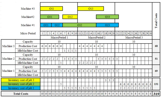
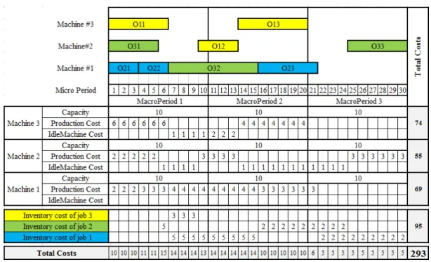
In the PLSP model the planning horizon consists of a finite number of periods. Machine capacities in each period are limited, andthey are different from period to period. For best utilization of each machine capacities, the remaining capacity can be used by another operation in same period. Inventory costs are different for each job and different from period to period. As an example for PLSP,in Figure 1, each job is assumed to have three operations and can be processed by three machines. Planning horizon consists of 3 periods and each period consists of 10 time units. As can be seen in Figure 1,solving the general FJSP with limited machine capacities leads to makespan of 21 unit time and total costs of 319. Adding inventory and idle machine costs in Figure 2, increases the makespan to 30 and the total costs decrease to 293.
75
Figure 2. PLSP Scheduling example whit costs objective
In the proposed PLSP modelthe other assumptions are made following: 1) Planning horizon is constant and finite.
2) All machines are continuously available from time zero
3) Demand rates, production rates, Idle Machine cost rates, Production cost rates, and inventory holding costs rates are deterministic and not constant over the planning horizon. 4) A machine can only execute one operation at a time.
5) External demands occur only for end operation of jobs.
6) Processing time rates are different for different products and different machines. 7) Production may be continued indefinitely without interruption.
8) Setup time is connivance.
9) Objective is to minimize the total costs. 10) Shortage is not allowed.
The indices of the model are: index of machine, = 1, … , index of jobs, = 1, … ,
ℎ index of operations, ℎ = 1, … , index of period, = 1, … , The parameters of the model are:
Sum of periods (Macro period*Micro period) Number of machines
Number of jobs
, Operation ℎ of Job
, , Processing time of operation , on machine
, Demand of job in the end of period
, Available capacity of machine in period
, Production coefficient, which indicates how many units of item produced through operation
76
, , If operation , can be processed on machine , is equal to one; otherwise, it is equal to zero
, , Cost of one unit inventory holding for operation , in period
, Cost of unit idle time for machine in period
Cost of one unit production for operation , on machine The variables of the model are:
, , , 1 : If operation 0 : otherwise , processed on machine in period
, , , Lot size of operation , on machine in period
, , Inventoryof operation , in the end of period
, Idle time of machine in period
The problem’s mixed integer programming model is as follows:
! " #$ = % % % , , ∗
' ( ) ( * (
+
ℎ + % % % % , , , ∗ , ,' ( ( * ( -( + % % , ∗ , ' ( -( (1) +. : , , = , , / + % , , , − % , ∗ , , , -( -(
= 1, … , ; ℎ = 1, … , − 1;
= 1, . . , ; , ,2= 0 (2)
,), = ,), / + % , ,), − ,
-(
= 1, … , ; = 1, . . , (3)
, / , / + % , , / , -( ≥ % , / ∗ , , , -(
= 1, . . , ; = 1, … , ;
ℎ = 2, … , ; , / ,2= 0 (4)
% % , , / , ' ( -( = % % , / ∗ , , , ' ( -(
= 1, . . , ; ℎ = 2, . . , (5)
% % , ,), ' ( -( = % , ' (
= 1, . . , (6)
, , , ∗ , , ≤ , ∗ 7 , , , / + , , , 8
= 1, . . , ; = 1, … , ; ℎ = 1, … , ; = 1, . . , ;
, , ,2 = 0
(7) % % , , , ∗ , , ) ( * (
≤ , = 1, . . , ; = 1, . . , (8)
, , , ≤ , , ℎ = 1, … , ; = 1, . . ,= 1, . . , ; = 1, … , ; (9)
% % , , , ) ( ≤ 1 * (
77
% , , ,
-(
≤ 1 = 1, … , ; ℎ = 1, … , ;= 1, … , (11)
, ≥ , − % % , , , ∗ , ,
) ( * (
= 1, . . , , = 1, … , (12)
, , , ∈ :0,1;
, , , ≥ 0
, , ≥ 0
, ≥ 0
= 1, . . , ; = 1, … , ;
ℎ = 1, … , ; = 1, . . , (13)
Equation (1) indicates the objective function, i.e. the total cost which includes the inventory cost, production cost and machine idle cost. Constraint (2) determines the inventory of operation , in the each period and shows the inventory balance between the micro periods, for all operations of each job except the last operation of each job. As for the last operation of each job, constraint (3) controls the inventory of job in the end of period to meet the demand. Constraint (4), (5) controls to quantity of operation , in the each period. Constraint (6) ensures the quantity of the last operation of job in all machines and all periods meet demand job in all periods.
Constraint (7) ensures that if possible, unused capacity of machine in each period is used. This constraint allows production variables to take non-zero values only if a machine is set up to process a given product in the current or previous period. In the PLSP at most two items of different types of items can be produced in each period. The first item produced in period corresponds to the second item produced in period − 1. For the second item the machine is going to be set up in period after a number of time units proportional to the time used for producing the first item. The splitting of the machine capacity for the production of two products within one period proportional to the quantities needed motivates the name of the model. (For further details about the PLSP models, refer to Drexl & Haase (1995) and Kaczmarczyk (2011)).
Constraint (8) ensures that the sum of work processing times on one machine in a specified period should not exceed the capacity of the machine in that period. Constraint (9) determines the feasibility of assigning operation , to machine , in other words, an operation can be processed on a machine only if that machine is capable of processing that operation. Constraint (10) assigns the operations to a machine in each period. Constraint (11) emphasizes that each operation can be performed only on one machine in each period. Constraint (12) determines the idle time of machine . Constraint 13 describes the decision variables.
4- Proposed algorithm for solving the problem
In this section first we present the basic Harmony Search algorithm. Then the difference between HS and mHs algorithm is described. Next, the method used for coding and decoding of the chromosomes is explained. Since all meta-heuristics algorithm start with an initial population, the mechanism for its generatingis explained. Finally, we proposed a new method to improvise a new harmony that enhances accuracy and convergence rate of harmony search (HS) algorithm.
4-1- Basic Harmony Search algorithm
Harmony search (HS) algorithm is a recently developed algorithm, and it is based on natural musical performance processes that occur when amusician searches for a better state of harmony, such as during jazz improvisation.In the classic harmony search (HS), the common parameters are the harmonymemory size (HMS), harmony memory consideration rate (HMCR), pitch adjusting rate (PAR), distance bandwidth (BW) and a stopping criterion (Geem et al., 2001).
78 4-1-1- Initialize the harmony memory
At first HM filled by HMS randomly generated harmony vectors. ! = :< , <= , . . . , <>;
Let< = :< (1), < (2) , . . . , < ("); represent the harmony vector in the HM, which is generated asfollows:
< (A) = B (A) + C ∗ 7D (A) − B (A)8 EFA = 1,2, … . . , " " = 1,2, … … , ! (14) Where LB(k) is a lower bound and UB(k) is an upper bound for decision variable < (A), and R is a random number between 0 and 1(Wang et al., 2011).
4-1-2- Improvise a new harmony
Improvisation is the process of generating a new harmony vector
<>GH = :<>GH(1), <>GH(2), … . . , <>GH("); in HS algorithm. <>GHis produced based on the following
rules (i.e. improvisation)(Wang et al., 2011).
4-1-3- Update harmony memory
Harmony memory is updated by comparing the new harmony (<>GH) with the worst harmony vector (<H). If <>GH is better than the <H, then <>GH replaces <H, and becomes a new member of the HM (Wang et al., 2011).
4-1-4- Check stopping criterion
If the stopping criterion (e.g. maximum number of improvisations, or maximum computational time) is reached, the computation is terminated. Otherwise, Sections 4.4.2 and 4.4.3 are repeated.
4-2- Harmony Search and Modified Harmony Search
The proposed approach for solving the problem is based on three major steps: 1) Determining the lot size of each operation in the period(s). 2) Assigning the operations to an appropriate machine. 3) Determining the sequence of operations in each period.
In the classic HS algorithm, generation of a New Harmony vector for all 3 steps above, is combined into a single step. This is wrong since it limits part of the solution space. In the proposed mHS algorithm, two vectors are improvised: the firstis Lot size-Machine vector and the second is sequence vector. This method will enhance the algorithm’s exploration ability.
Thus, the mHS and the HS are different in two aspects as follows:
1) The mHS improvised a New Harmony vector in two phases to enhance search ability. In the first phase, a new harmonyvector lot size-machine assignment for each job and in the last phase, a New Harmony vector sequence is generated.
2) Furthermore, inspired by the swarm intelligence of particle swarm, mHS modifies the improvisation step of the HSby a matrix called the “Repetition Matrix “ which is explained in details in section 4.6.3
Figure 3 shows the schematic of the proposed mHS for integrated lot size andscheduling in a flexible job shop problem. In the following, the proposed Harmony Search algorithm is fully described.
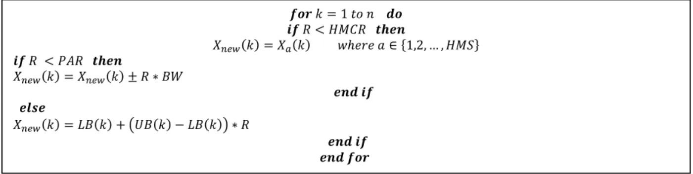
IJK A = 1 E " LJ MI C < ! C OPQR
<>GH(A) = <S(A) Tℎ$F$ ∈ :1,2, … , ! ;
MI C < UC OPQR
<>GH(A) = <>GH(A) ± C ∗ W
QRL MI QXYQ
<>GH(A) = B (A) + 7D (A) − B (A)8 ∗ C
QRL MI QRL IJK
79 4-3- Coding of Chromosomes
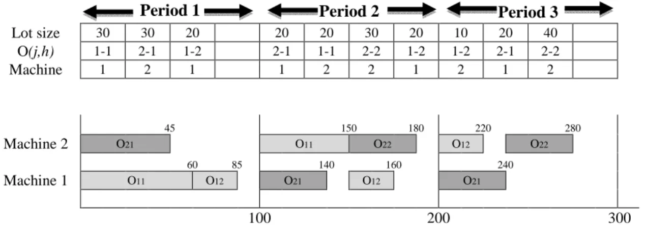
For encoding of chromosomes, a matrix with three rows and !. Z. columns is used in which ! is the number of machines, Z is the number of production positionsfor each machine in every period, and is the number of periods throughout the planning horizon. This method is adapted and modified from Rohaninejad (2015b). In this matrix, the elements of the first row indicate the quantities of items that are produced through operation ( , ℎ) in period which are equal to units. The elements of the second row include two components ( , ℎ)which indicate the operation ℎ of Job . In other words, the second row shows the sequence of different operations. Third row of the matrix represents the machine assignments made to elements of the second row. As an example, Figure 4 shows a chromosome for two jobs, each consists of two operations which should be processed on two machines in a planning horizon that spans three periods.
Period 1 Period 2 Period 3
Lot size 30 30 20 20 20 30 20 10 20 40
O(j,h) 1-1 2-1 1-2 2-1 1-1 2-2 1-2 1-2 2-1 2-2
Machine 1 2 1 1 2 2 1 2 1 2
80
Start
Step1 Initialization of an optimization problem and algorithm
parameters
For minimizing objective function (cost)
Specification of each decision variable, a possible value range in each decision variable, harmony memory size (HMS), harmony
memory considering rate (HMCR), pitch adjusting rate for Lot size and Machine and pitch adjusting rate for Sequence (PARLM,PARS), An arbitrary distance bandwidth for Lot size
and Machine and bandwidth for Sequence (BWLM,BWS) termination criterion (maximum number of search)
Step2 Initialization of harmony memory
(HM) Generation of initial
population
(Section 4.5)*
Step 3
Improve a new harmony from HM
Sorted HM by Cost
Rand()<HMCR
(Se 4.6)
Rand()<PARLM
(Se 4.6)
For all iterate
Pitch adjusting Sequence
(Se 4.6.3)
Memory Consideration
(Se 4.6)
Pitch adjusting Lot size and Machine
allocate
(Se 4.6.1 & 4.6.2) No
Yes
Yes
New Random Lot size and Machine
allocate
(Se 4.5.3 & 4.5.4) No
Rand()<PARS
(Se 4.6) Yes
New Random Sequence
(Se 4.5.2)
No
A new harmony is better than a stored
Harmony in HM?
(Se 4.7)
Termination criterion satisfied?
Stop
No
Yes
Updating HM
(Se 4.6) Yes
No
BWLM
BWS
Figure 3. Schematic of the modified Harmony Search in PLSP
81 4-4-Decoding of chromosomes
In this section, the start time of an operation, the processing duration of that operation, and the machine availability should be considered. The start time for an operation is the maximum time of machine availability and the time when the required inventory is provided. Also, the processingtime duration of operation , will be equal to , . , when operation , has been assigned to machine .Figure 5 shows the manner of decoding of chromosome.
Period 1 Period 2 Period 3
Lot size 30 30 20 20 20 30 20 10 20 40
O(j,h) 1-1 2-1 1-2 2-1 1-1 2-2 1-2 1-2 2-1 2-2
Machine 1 2 1 1 2 2 1 2 1 2
45 150 180 220 280
Machine 2 O21 O11 O22 O12 O22
60 85 140 160 240
Machine 1 O11 O12 O21 O12 O21
100 200 300
Figure 5.Manner of decoding of chromosome
In figure5, operation , is processed for 60 time units, because the value of , is assumed to be equal to 2in the first period. Furthermore, it can be seen that the values of =, , =, and =,= are assumed as 2.5, 2.0 and 1.5, respectively. Also, the coefficient of utilization of product from operation
= in the product of operation == is assumed as1.0 (Rohaninejad et al., 2015b). 4-5- Generating the initial population of the algorithm
According to above, the generation of the initial population is based on the following four steps. 4-5-1- Determining the production periods for each item
In this step, the production periods for each item are selected randomly and all the periods have an equal chance ofbeing selected. In order to prevent shortage, the selection of the first production period for each item is a function of the first period where there is a demand for that item (Rohaninejad et al., 2015b).
4-5-2- Determining the sequence of operations which are assigned to a period
For determining the sequences of operations assigned to a specificperiod, arandom method is borrowed form Rohaninejad (2015b). In this approach, from the operations assigned to a period, one operation is randomly selected and entered into the first unplanned sequence priority of that period.Moreover, in the first period, in order to prevent having a shortage, no operation is planned unless the previous operation is done.
4-5-3- Determining the lot size values for each operation
In this step, we use the procedure that Rohaninejad (2015b) presented for simultaneous lot-sizing and scheduling in flexible jobshop problems. In this procedure, the production quantity of operation ,[ item in sequence + is equal to:
,
\] =
, + C " (^, − ∆, + ∑\(\]/ , . \, − , ). (15)
Rand is random number between 0 and 1, and ^, is the total demand for the item ( , ) of operation during the planning horizon and ∆, is difference between total production and total consumption of the item produced in operation , prior to sequence + .(Rohaninejad et al., 2015b).
82 4-5-4- Assigning machines to operations
To assign a machine to an operation, one of the allowed machines is randomly assigned toeach operation.
4-6-Proposed New Harmony algorithm for PLSP
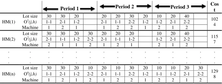
In this paper, an initial population of harmony vectors are generated according to section 4.3 and stored in the harmony memory (HM). There are four segments in the HM: lot size of operation , , machine assignment matrix, sequence of job operations and finally evaluation of total cost. Figure 6 presents the structure of the proposed harmony memory. It is noteworthy that HM should be sorted by cost.
According to above, a New Harmony vector <>GH has three parts: harmony vector lot size for each operation( >GH), harmony vector machine assignment(!>GH), and harmony vector sequence ( >GH).
Period 1 Period 2 Period 3
Cos t HM(1)
Lot size 30 30 20 20 20 30 20 10 20 40 102
4 O1(j,h) 1-1 2-1 1-2 2-1 1-1 2-2 1-2 1-2 2-1 2-2
Machine 1 2 1 1 2 2 1 2 1 2
HM(2)
Lot size 30 30 20 30 20 20 20 10 20 40
115 7 O2(j,h) 2-1 1-1 1-2 2-2 2-1 1-1 1-2 1-2 2-1 2-2
Machine 2 1 1 2 1 2 1 2 1 2
. . . .
. . . .
. . . .
HM(n)
Lot size 30 30 20 10 20 10 30 20 10 10 20 30 129
8 On(j,h) 1-1 2-1 1-2 2-2 2-1 1-1 2-2 1-2 1-1 1-2 2-1 2-2
Machine 1 2 1 2 1 2 2 1 2 2 1 2
Figure 6. Scheme of harmony memory structure
A New Harmony vector, <>GH generated from the HM based on memory considerations, pitch adjustments, and randomization, is shown in Figure 3. Computational procedure for the mHS can be summarized as follows:
Step 1: Set the parameters, ! , ! C, UCB!, UC , WB!, W and the termination criterion.
Step 2: Initialize the HM and calculate the objective function value for each harmony (section4.3). Step 3: Improvise a New Harmony vector <>GH : We improvise a New Harmony vector in two phases to enhance searching ability. In the first phase, generate a New Harmony vector lot size( >GH), and machine assignment(!>GH) for each job. In the second phase, generate a New Harmony vector sequence( >GH). In other words, either the lot size for a job does not change so it comes straight from the harmony memory, or a new vector is generated for each job. A similar procedure is done for the machine assignment as well. Once all the lot sizes and machine assignments are determined, a new sequence vector could be generated. Thus, a New Harmony vector lot size( >GH), and machine assignment(!>GH) are proposed in the following pseudo code:
83
And, improvise a New Harmony vector sequence( >GH) with following pseudo code:
F1, F2, … . , F10 is random number between 0 and 1.
Step 4: Update the HM as, <H = <>GH ; if E+ (<H) < E+ (<>GH)
Step 5: If the given termination criterion is satisfied, return the best harmony vector in the HM; otherwise go to Step 3.
We can easily add a local search to the mHS algorithm in order to enhance its exploration ability. This can be done by improving each candidate harmony vector generated in the improvisation phase. There are three types of neighborhoods that can be employed in the local search: the first is based on lot size, the second is based on machine assignment and the third is based on a job permutation.
4-6-1- Pitch adjusting lot size
Pitch adjusting of a lot size can be obtained by increasing or decreasing the quantity of lot size. Since the converting process is needed for fitness evaluation, lower and upper bounds for lot sizes of each job should be calculated. In other words, to prevent the shortage, the band width of the lot size is obtained from the following procedure:
According to section 4-5-3, this procedure starts from the first period and continues to the last. The lot size upper bound is the maximum quantity of theitem produced during the operation ,[, that is F, . Similarly, thelot size lower bound is the minimum quantity of theitem produced during the operation ,[, that is , . Finally, a band width of lot size in sequence + is equal to:
W \,] = ^
, − ∆, + ∑\\(]/ , . \, − , (16)
Thus, A Pitch adjusting of a lot sizein sequence + is equal to:
>GH(A) = >GH(A) ± C " ∗ W ∗ W \,](A), (17)
Where W is Bandwidth Quantity Index.In this equation Rand is random number between 0 and 1, and ^, is the total demand for the item ( , ) of operation during the planning horizon and ∆, is difference between total production and total consumption of the item produced in operation , prior to sequence + .
aJK(A = 1 E ")LJ MI(F9 < UC )OPQR
>GH(A) = >GH(A) ± F9 ∗ Wc(A)
QXYQ MI
>GH(A) = B d(A) + F10 ∗ (D d(A) − B d(A))
QRL MI QRL IJK
aJK( ee E ) LJ aJK(A = 1 E ")LJ MI(F1 < ! C)OPQR
>GH(A) = S(A) Tℎ$F$ ∈ (1,2, … ! )
!>GH(A) = !S(A) Tℎ$F$ ∈ (1,2, … ! )
MI(F2 < UCB!)OPQR
>GH(A) = >GH(A) ± F3 ∗ Wd(A)
!>GH(A) = !>GH(A) ± F4 ∗ Wh(A)
QXYQ MI
>GH(A) = B d(A) + F5 ∗ (D d(A) − B d(A))
!>GH(A) = B h(A) + F6 ∗ (D h(A) − B h(A))
QRL MI QXYQ MI
>GH(A) = B d(A) + F7 ∗ (D d(A) − B d(A))
!>GH(A) = B h(A) + F8 ∗ (D h(A) − B h(A))
QRL MI QRL IJK QRL IJK
84 4-6-2- Pitch adjusting machine assignment
A pitch adjusting of a machine assignment is performed by assigning/not assigning a machine to an operation ,[in each period. Thus, a band width of machine assignment for job is the number of machines that can be used in period .
A pitch adjusting of a machine assignment is equal to:
!>GH(A) = !>GH(A) ± C " ∗ W ! ∗ W!(A) ,
(18)
Where W ! is Bandwidth Machine Index. 4-6-3- Pitch adjusting sequence
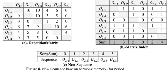
A neighbor for a job permutationcan be obtained by INSERT, INVERSE or SWAP operators (Pinedo, 2012).The local search in the mHS algorithm is not directly applied to the position of the candidate harmony vector but to the job permutation implied by the candidate real vector. In this method the candidate real vector is achieved by maximum repeat rate of operation , in harmony memory. To determine the new sequence, the number of operation ( , ) which is achieved after operation ( m, m) in all harmony memory sequence vector is considered, and stored in the Repetition Matrix. Thus, Tn,o in Repetition Matrix is number of q that performed after p, wherep " ∈ , .
Thus a New Harmony sequence vector, with following pseudo code is improvised:
Furthermore, figure 7 presents the scheme of scheduling in harmony memory. In this case HMS is 10 and harmony sequence vectors are composed of two periods, two jobs and three operations. RepetitionMatrix is created by the number of repetition a pairwise comparison of operation with each other yields (Figure 8). Matrix Index array in Figure 8 is calculated by the above pseudo code. The sum of column array in Matrix Index is rate of( , ), and it seeks to find the best sequence. To find the new sequence, sum of column array in matrix index should be sorted, to find the best sequence in period 1. And this procedure should be continued for each period. See Figure 8(c)
Period 1 Period 2
HM(1) O1(j,h) 2-1 1-1 2-2 1-2 1-3 2-3 1-3 2-3
HM(2) O2(j,h) 2-1 2-2 1-1 2-3 1-2 1-3 2-2 2-3 HM(3) O3(j,h) 1-1 2-1 1-2 1-3 2-2 2-3 2-2 2-3 HM(4) O4(j,h) 1-1 1-2 2-1 2-2 1-3 2-3 2-1 2-2 1-3 2-3 HM(5) O5(j,h) 2-1 2-2 1-1 2-3 1-2 1-3 2-1 2-2 2-3 HM(6) O6(j,h) 2-1 2-2 1-1 2-3 1-2 1-3 2-2 2-3 HM(7) O7(j,h) 2-1 1-1 1-2 2-2 2-3 1-3 1-1 1-2 1-3 2-3 HM(8) O8(j,h) 2-1 2-2 1-1 1-2 2-3 1-3 2-2 2-3 1-3 HM(9) O9(j,h) 1-1 1-2 1-3 2-1 2-2 2-3 2-1 2-2 2-3 HM(10) O10(j,h) 1-1 1-2 2-1 2-2 1-3 2-3 1-1 1-2 1-3
Figure7. Scheme of Scheduling in harmony memory IJK $ qℎ $F E
rPMXQ ! s ≠ 0
! s = ! s u Tn,o ; Tℎ$F$ Tn,o ∈ ! F s C$p$
un,o= 1 , Tℎ$F$ un,o ∈ ! F s " $s
Tn,o= To,n= 0
MI u,n= 1; ℎ$" u,o= 1 " T,o= To, = 0 ; QRL; EF ee ∈ p
MI uo, = 1; ℎ$" un, = 1 " Tn, = T,n= 0 ; QRL; EF ee ∈ p
QRL rPMXQ o= % u,o
n
(
"$T +$ u"q$ = +EF o
85 4-7- Calculate the objective function
In this paper, the objective function is to minimize the total cost which includes the inventory cost, production cost and idle costs ofmachines. Production cost, can easilybe calculated according to equation 1. Idle costs and Inventory costs are related to start and finish time of operations in the sequence. According to section 4.2, the start time of an operation depends on the time the required inventory is provided to start processingthe operation. Machine availability time and sufficient inventory are necessaryfor the start of operation, thus the maximum of these two factors is the start time for the operation. Hence, the start time, finish time, and inventory of operation( , ), can be obtained with the following pseudo code:
, ,= ,v =, =,= =,v
, 1 1 0 1 1
,= 0 1 0 0 1
,v 0 0 0 0 0
=, 1 1 1 1 1
=,= 0 1 1 0 1
=,v 0 0 1 0 0
Sum 1 3 5 0 2 4
(b)-Matrix Index
Sort(Sum) 0 1 2 3 4 5
Sequence =, , =,= ,= =,v ,v
(c)-New Sequence
Figure 8. New Sequence base on harmony memory (for period 1)
wI7 ", / > , 8OPQR; T ℎ y z$" qE"+u p E" F $ , = U (! )
{ , = , + , ∗ ,
QXYQ MI
MI!m( , / ) = ! ( , ) OPQR , = U (! )
{ , = , + , ∗ ,
QXYQ MI
e = max7{ •, •/ , , / 8 ; Tℎ$F$ •, •/ +pF$Ep$F E" , " qℎ "$ MI7e = { •, •/ 8OPQR
, = e
QXYQ MI
, = , / + 1
QRL MI
z, / = ", / + "(7{ , / − , / 8 , 7 , − , / 8)/ , /• ; ′ ∈ !( , / )
MI z, / ≥ , OPQR
{ , = , + , ∗ , ; ∈ !( , )
QXYQ MI
MI , /m ≤ , OPQR
{ , = , + , ∗ ,
QXYQ MI
MI z, / ≤ , ∗ 71 − , ‚ , /• 8OPQR
{ , = { , / + ,
QXYQ MI
{ , = , + , ∗ ,
QRL MI QRL MI QRL MI QRL MI QRL MI
, ,= ,v =, =,= =,v
, 10 10 4 6 0
,= 0 10 3 5 0
,v 0 0 1 2 0
=, 6 7 9 10 6
=,= 4 5 8 0 4
=,v 0 3 5 0 0
86
Here, , is the duration of processing time of , on machine and , is the lot size , , ", is the inventory , , , is the start time of , ,{ , is the finish time of , , and At is the availably time. Thus, inventory costs and idle costs can be calculated.
5-Computation results
5-1- Generating random instances for the problem
Since there is no dataset for this problem (lot size and scheduling of jobs in a flexible environment), it is necessary to generate random instances for the problem in order to evaluate and compare the performance of the proposed algorithm, with the optimal method (Rohaninejad et al., 2015b). We consider different problem sizes as is shown in Table 1.
Finally, 18 instances with the Table 1 conditions are generated in small, mediumand large sizesand each instance is labeled with (ƒ, „, …, †), which ƒ indicates the number of jobs,„ indicates the total number of operations,… indicates the number of machines and †is the number of periods in the planning horizon (Rohaninejad et al., 2015b).
Table 1. Manner of generating random instances
Parameter Notation Generated by
Demand quantities of every job , Normal distribution with the average round (2. Z ) and variance 2. (NT is the number of macro period).
Length of each period B
Normal distribution with the average (3. . /2) and variance M. (O denotes the total number of operations, M is the number of machines, and J is the number of jobs)
Fixed loss of time for production
unit of items , , Uniform distribution between [0.1-0.5] Production costs , , Uniform distribution between [0.2-1] Idle costs , Uniform distribution between [0.1-0.5] Holding costs , , Uniform distribution between[1-4] Production coefficient , 1
5-2- Parameters calibration
In this paper, the Taguchi method is applied for calibration the parameters of the proposed harmony search algorithm. Taguchi in early 1960s has proposedthis method. The concept of Taguchimethod is based on maximizing a performance measure called signal-to-noise ratio by running a partial set ofexperiments using the orthogonal arrays (Wu & Hamada, 2011). S/N ratio is calculated as follows:
c
‡F E = −10log (‡∑>( ‹Œ•)(19)
Where and " denote the response variables and number of replications, respectively. We consider 4 factors that can have significant effect on the algorithm. These factors and their levels are shows in table 2.
Table 2. Factors and their levels for New HS algorithm
Factor Levels Number of levels
HMCR (Harmony Memory Consideration Rate) {0.1;0.3;0.5;0.7} 4 PARLM (Pitch Adjustment Rate for Lot size and
Machine assignment) {0.2;0.3;0.4;0.5} 4
PARS (Pitch Adjustment Rate for Sequence) {0.2;0.3;0.4;0.5} 4 BWLM (Bandwidth Lot size and Machine index) {0.2;0.4;0.6;0.8} 4
The lower the better, the higher the better, and the nominal the better are three type of quality characteristics in the analysis of the S/N ratio (Wu & Hamada, 2011).In this paper, the S/N ratio for the larger the better characteristic is calculated.
The Taguchi design of mHS algorithm isB Ž(4•). The selected Taguchi design has 16 different combinations of parameter levels. For every trial, three random instances (two small size andone medium size) are considered and each of themis replicated six times in order to obtain more reliable results. The mean response variable is calculated as follows:
87
$q z$, =(∑ •‘ G’ “GŒ,”,•
–
•—] ⁄ )/h >Ž Œ
h >Π(20)
Where indicate the instance index ( = 1, … ,3)and indicate the trial number ( = 1, … ,16) and A the reapplication number (A = 1, … ,6).The E $q z$ value is converted in to S/N ratio. Figure 9 show the mean S/N ratio for each level of control factors in mHS algorithm.
For the analysis of variance (ANOVA), factors are considered as control factors and thelevels with largest values of S/N ratio are selected as the optimal value for each of them. Theoptimal level for factors in Table2 are 0.3, 0.2, 0.5 and 0.4 from top to bottom. Other parameters are shown in table3.
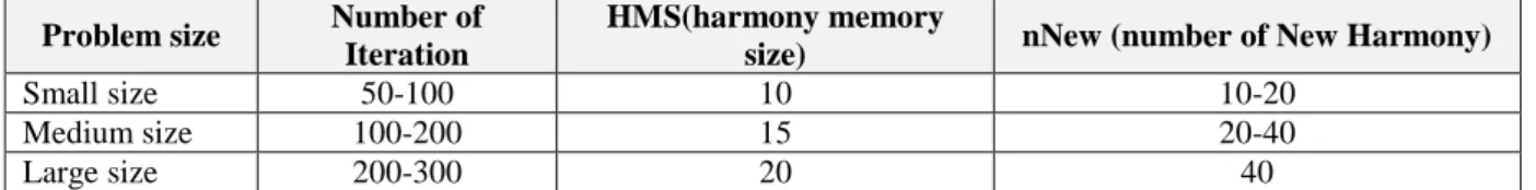
Table 3. The parameter of mHS algorithm Problem size Number of
Iteration
HMS(harmony memory
size) nNew (number of New Harmony)
Small size 50-100 10 10-20
Medium size 100-200 15 20-40
Large size 200-300 20 40
5-3- Comparison and Evaluation of the Proposed Solution Methods
In this section, the performance of HS and mHs for solving the considered problem with Matlab 8.3 software is investigated andthe results are compared with the exact solutions found by CPLEX 12.6 solver. The experiment is run on a PC with 2.2GHz processor and 8GB of RAM. The obtained results of solving the small,medium and large size instances are listed in Tables 4 to 6 respectively.
0.7 0.5 0.3 0.1 36
34
32
0.5 0.4 0.3 0.2
0.5 0.4 0.3 0.2 36
34
32
0.8 0.6 0.4 0.2 HMCR
M
e
a
n
o
f
S
N
r
a
t
io
s
PARLM
PARS BWLM
Main Effects Plot for SN ratios
Data Means
Signal-to-noise: Larger is better
Figure9. The mean S/N ratio plot for each levelof the factors in mHS algorithm
88
To evaluate the performance, this criterion will be used:™ pS=š‘’G “Gœ•ž(š‘’G “G)›/œ•ž(š‘’G “G) (21) The computation time of the HS and mHS are smaller than the exact method. Also, in cases where the CPLEX software has not reached the optimal solution after3600 s of computation time, mHS achieves a better solution. The total cost for mHS algorithm is smaller than those HS and exact methods. Thus, the mHS has a better performance for all problem sizes.
A general review of the results in Table 4,5 and 6 shows that:
The HS method can only solve small size problems and also needs more computational time to solve these test problems.
The mHS algorithm can solve all the test problems.
The mHS has the ability to obtain solution for all test problems.
The mHS can find good quality solutions for all size problems. The objective values obtained by mHS are better from HS and exact method results.
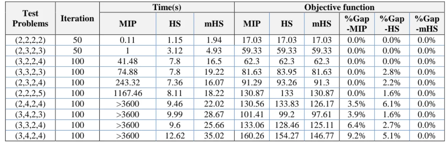
Table 4. Details of computational results for small size instance
Test
Problems Iteration
Time(s) Objective function
MIP HS mHS MIP HS mHS %Gap -MIP
%Gap -HS
%Gap -mHS (2,2,2,2) 50 0.11 1.15 1.94 17.03 17.03 17.03 0.0% 0.0% 0.0% (2,3,2,3) 50 1 3.12 4.93 59.33 59.33 59.33 0.0% 0.0% 0.0% (3,2,2,4) 100 41.48 7.8 16.5 62.3 62.3 62.3 0.0% 0.0% 0.0% (3,3,2,3) 100 74.88 7.8 19.22 81.63 83.95 81.63 0.0% 2.8% 0.0% (2,3,2,4) 100 243.32 7.36 16.07 91.29 93.26 91.3 0.0% 2.2% 0.0% (2,2,2,5) 100 1167.46 8.11 18.22 130.87 133 130.87 0.0% 1.6% 0.0% (2,4,2,4) 100 >3600 9.46 22.02 130.56 133.83 126.17 3.5% 6.1% 0.0% (3,4,2,3) 100 >3600 9.99 28.67 101.41 99.2 97.61 3.9% 1.6% 0.0% (3,3,2,4) 100 >3600 9.6 25.66 133.06 128.46 125.11 6.4% 2.7% 0.0% (3,4,2,4) 100 >3600 12.62 35.02 160.26 154.27 146.77 9.2% 5.1% 0.0%
Table 5. Details of computational results for medium size instance
Test
Problems Iteration
Time(s) Objective function
MIP
HS mHS MIP HS mHS %Gap -MIP
%Gap -HS
%Gap -mHS
R B
(4,4,3,4) 100 >3600 1170 24.32 79.62 291.79 302 280 4% 8% 0%
(4,4,3,6) 100 >3600 576 23.48 75.81 1141.2 634.08 589.79 93% 8% 0%
(4,5,3,5) 150 >3600 1564 57.93 250 --- 580.34 550.14 --- 5% 0%
(4,6,4,5) 150 >3600 2536 76.39 335 602.76 611.06 570.6 6% 7% 0%
(4,7,4,5) 150 >3600 700 94.26 580 1079.6 991.53 876.43 23% 13% 0%
Table 6. Details of computational results for large size instance
Test
Problems Iteration
Time(s) Objective function
MIP
HS mHS MIP HS mHS %Gap -MIP
%Gap -HS
%Gap -mHS
R B
(5,8,5,6) 200 >3600 2978 231.2 1224 1817.2 1726.4 1640.8 11% 5% 0%
(8,9,6,6) 200 >3600 --- 583.38 3083 --- 1902.8 1782.2 --- 7% 0%
(9,9,7,6) 200 >3600 --- 824.37 4585 --- 2243.7 2004.3 --- 12% 0%
In tables 5 and 6, R is real time needed to solve MIP Problem with Cplex solver and B is the best time to find the best feasible solution in PC with 2.2 GHz Processor and 8Gb of RAM. (Because this problem is NP-Hardand Cplex cannot solve this size problem).
Comparing the CPU times of exact solution confirms that computation timegrows exponentially by increasing the dimension of the problem. The presented heuristics and meta-heuristicalgorithms can
89
find the optimal solution for small size problems.The computation time of the HS andmHS are smaller than the exact method.By comparing the proposed algorithms, it is concluded that the mHS algorithm has a moreconvincing performance than other solutions.
6- Conclusion and future research directions
This paper proposed an integrated lot sizing and flexible job shop scheduling problem with machine capacity constraints to minimize the total cost; including the inventory, idle machine and production costs.A new mixed integer programming model, with small bucket time approach, based on Proportional Lot sizing and Scheduling Problems (PLSP), is proposed to formulate the problem. In order to solve the problem, a New Harmony search algorithm had been developed.In this method, we improved a New Harmony vector in two phases to enhance search ability. In the first phase, a New Harmony vector lot size-machine assignment for each job and in the last phase, a New Harmony vector sequence is generated.The performance of the proposed algorithm was compared with the exact method and the classic harmony search algorithm in small, medium and large size problems. Computational results and comparisons demonstrated the effectiveness and efficiency of the proposed algorithm.The proposed algorithm can find good quality solutions for all size problems. The objective values obtained by proposed algorithm are better from HS algorithm and exact method results.
This approach can be used in the solving of other problemsof simultaneous optimization of lot-size and scheduling. As for the future work, the model can be extended to include the maintenance periods, the remaining work in the sequence and thelatest time of machines’ availability in machine assignment.
References
Adetunji, O. A. B., &Yadavalli, V. (2012). An integrated utilisation, scheduling and lot-sizing algorithm for pull production.International Journal of Industrial Engineering: Theory, Applications and Practice, 19(3).
Akrami, B., Karimi, B., &Hosseini, S. M. (2006). Two metaheuristic methods for the common cycle economic lot sizing and scheduling in flexible flow shops with limited intermediate buffers: The finite horizon case. Applied Mathematics and Computation, 183(1), 634-645.
Almada-Lobo, B., & James, R. J. (2010). Neighbourhood search meta-heuristics for capacitated lot-sizing with sequence-dependent setups.International Journal of Production Research, 48(3), 861-878.
Beraldi, P., Ghiani, G., Grieco, A., &Guerriero, E. (2008). Rolling-horizon and fix-and-relax heuristics for the parallel machine lot-sizing and scheduling problem with sequence-dependent set-up costs.Computers & Operations Research, 35(11), 3644-3656.
Drexl, A., &Haase, K. (1995).Proportional lotsizing and scheduling.International Journal of Production Economics, 40(1), 73-87.
Fandel, G., &Stammen-Hegene, C. (2006).Simultaneous lot sizing and scheduling for multi-product multi-level production.International Journal of Production Economics, 104(2), 308-316.
Fattahi, P., Jolai, F., &Arkat, J. (2009).Flexible job shop scheduling with overlapping in operations.Applied Mathematical Modelling, 33(7), 3076-3087.
Fattahi, P., Mehrabad, M. S., &Jolai, F. (2007). Mathematical modeling and heuristic approaches to flexible job shop scheduling problems. Journal of Intelligent Manufacturing, 18(3), 331-342.
Gao, K. Z., Suganthan, P. N., Pan, Q. K., Chua, T. J., Cai, T. X., & Chong, C. S. (2014). Discrete harmony search algorithm for flexible job shop scheduling problem with multiple objectives.Journal of
90 Intelligent Manufacturing, 1-12.
Geem, Z. W., Kim, J. H., &Loganathan, G. V. (2001). A new heuristic optimization algorithm: harmony search. Simulation, 76(2), 60-68.
Gómez Urrutia, E. D., Aggoune, R., &Dauzère-Pérès, S. (2014). Solving the integrated lot-sizing and job-shop scheduling problem.International Journal of Production Research, 52(17), 5236-5254. Haase, K., &Kimms, A. (2000).Lot sizing and scheduling with sequence-dependent setup costs and times and efficient rescheduling opportunities.International Journal of Production Economics, 66(2), 159-169.
Kaczmarczyk, W. (2011).Proportional lot-sizing and scheduling problem with identical parallel machines.International Journal of Production Research, 49(9), 2605-2623.
Karimi, B., Ghomi, S. F., & Wilson, J. M. (2003). The capacitated lot sizing problem: a review of models and algorithms. Omega, 31(5), 365-378.
Karimi-Nasab, M., Seyedhoseini, S. M., Modarres, M., &Heidari, M. (2013). Multi-period lot sizing and job shop scheduling with compressible process times for multilevel product structures. International Journal of Production Research, 51(20), 6229-6246.
Kovács, A., Brown, K. N., &Tarim, S. A. (2009).An efficient MIP model for the capacitated lot-sizing and scheduling problem with sequence-dependent setups.International Journal of Production Economics, 118(1), 282-291.
Mahdieh, M., Bijari, M., & Clark, A. (2011).Simultaneous Lot Sizing and Scheduling in a Flexible Flow Line.Journal of Industrial and Systems Engineering, 5(2), 107-119.
Modrak, V. (2012). Alternative Constructive Heuristic Algorithm for Permutation Flow-Shop Scheduling Problem with Make-Span Criterion. International Journal of Industrial Engineering: Theory, Applications and Practice, 19(7).
Morais, M. D. F., GodinhoFilho, M., &Boiko, T. J. P. (2014). Hybrid flow shop scheduling problems involving setup considerations: a literature review and analysis. International Journal of Industrial Engineering: Theory, Applications and Practice, 20(11-12).
Petrovic, S., Fayad, C., Petrovic, D., Burke, E., & Kendall, G. (2008).Fuzzy job shop scheduling with lot-sizing.Annals of Operations Research, 159(1), 275-292.
Pinedo, M. L. (2012). Scheduling: theory, algorithms, and systems.Springer Science & Business Media. Ponnambalam, S. G., & Reddy, M. (2003). A GA-SA multiobjective hybrid search algorithm for integrating lot sizing and sequencing in flow-line scheduling.The International Journal of Advanced Manufacturing Technology, 21(2), 126-137.
Ramezanian, R., &Saidi-Mehrabad, M. (2013). Hybrid simulated annealing and MIP-based heuristics for stochastic lot-sizing and scheduling problem in capacitated multi-stage production system. Applied Mathematical Modelling, 37(7), 5134-5147.
Ramezanian, R., Saidi-Mehrabad, M., &Fattahi, P. (2013). MIP formulation and heuristics for multi-stage capacitated lot-sizing and scheduling problem with availability constraints. Journal of Manufacturing Systems, 32(2), 392-401.
91
search–firefly algorithms for the capacitated job shop scheduling problem with sequence-dependent setup cost. International Journal of Computer Integrated Manufacturing, 28(5), 470-487.
Rohaninejad, M., Kheirkhah, A., &Fattahi, P. (2015b). Simultaneous lot-sizing and scheduling in flexible job shop problems. The International Journal of Advanced Manufacturing Technology,78(1-4), 1-18.
Rohaninejad, M., Kheirkhah, A., Fattahi, P., &Vahedi-Nouri, B. (2015c).A hybrid multi-objective genetic algorithm based on the ELECTRE method for a capacitated flexible job shop scheduling problem.The International Journal of Advanced Manufacturing Technology, 77(1-4), 51-66.
Sikora, R., Chhajed, D., & Shaw, M. J. (1996).Integrating the lot-sizing and sequencing decisions for scheduling a capacitated flow line.Computers & Industrial Engineering, 30(4), 659-679.
Toledo, C. F. M., França, P. M., Morabito, R., &Kimms, A. (2009). Multi-population genetic algorithm to solve the synchronized and integrated two-level lot sizing and scheduling problem.International Journal of Production Research, 47(11), 3097-3119.
Wang, L., &Zheng, D. Z. (2001).An effective hybrid optimization strategy for job-shop scheduling problems.Computers & Operations Research, 28(6), 585-596.
Wang, L., Pan, Q. K., &Tasgetiren, M. F. (2010).Minimizing the total flow time in a flow shop with blocking by using hybrid harmony search algorithms.Expert Systems with Applications, 37(12), 7929-7936.
Wang, L., Pan, Q. K., &Tasgetiren, M. F. (2011).A hybrid harmony search algorithm for the blocking permutation flow shop scheduling problem.Computers & Industrial Engineering, 61(1), 76-83. Weidenhiller, A., &Jodlbauer, H. (2009). Equivalence classes of problem instances for a continuous-time lot sizing and scheduling problem. European Journal of Operational Research, 199(1), 139-149.
Wu, C. J., & Hamada, M. S. (2011). Experiments: planning, analysis, and optimization (Vol. 552). John Wiley & Sons.
Zhu, C. (2012). Applying Genetic Local Search Algorithm to Solve the Job-Shop Scheduling Problem.International Journal of Industrial Engineering: Theory, Applications and Practice, 19(9).