Modeling and Tracking of Crowded Traffic Scenes by using Policy Trees, Occupancy Grid Blocks and Bayesian Filters

Abstract—In this paper we propose a new solution for representing and tracking crowded traffic environments by using dense stereo data. The proposed method relies on the information provided by two compact 2.5D grid-based representations: a classified occupancy grid and an intensity grid. The measurement data is extracted using a predefined Policy Tree, which represents a path structure used to accelerate the object delimiter extraction. The extracted measurements are given in form of rectangular grid blocks that are described by three components: a dynamic, a geometry and an intensity component. We propose a medium level tracking approach in which the state is estimated for each block individually. To be able to work with a high dimensional state space a Rao-Blackwellized particle filter is used. The proposed solution has several advantages. First, the data association is performed at the particle level, thus being handled in a natural way by a weighting-resampling mechanism. Second, unlike other existing geometry-based solutions we also incorporate the intensity information in the tracking process. Finally, the proposed method takes into account the uncertainties of the stereovision system.

I. INTRODUCTION

Modeling and tracking of dynamic and crowded environments represents a difficult research task for any driving assistance system. Usually, the surrounding world of a moving vehicle is unknown and filled with many objects of different shapes, types, sizes and speeds. Moreover, in cluttered environments, such as urban traffic scenes, the representation module may be affected by occlusions, unpredictable behavior of the objects or introduced measurement noises. Therefore, the expectations from an advanced driver assistance system are high, as such a system should be able to use the imperfect sensorial information in order to accurately represent the driving world and to locate and track the relevant traffic entities.

The general problem of vision-based modeling and tracking of dynamic environments can be divided into several main subtasks: acquiring the measurement data, extracting a set of relevant entities by using specific representation models and keeping track of these entities over time. Many stereovision-based methods have been proposed in the literature. An extensive survey of the past

Andrei Vatavu, Radu Danescu and Sergiu Nedevschi are with the Technical University of Cluj-Napoca, Computer Science Department (e-mail: {firstname.lastname}@cs.utcluj.ro). Department address: Computer Science Department, Str. Memorandumului nr. 28, Cluj-Napoca, Romania. Phone: +40 264 401484.

decade’s progress in the vision based on-road object detection and tracking is presented in [1].

Current environment representation and tracking approaches can be split into two main categories: intensity-based solutions [3][10] and geometry-intensity-based solutions [4][8][9]. Usually, the intensity-based methods combine the depth information with the motion cues computed by optical flow. For example, in [10], the scene flow is computed by simultaneously extracting the stereo and motion information. In [3], the primary depth data is directly used to estimate the 3D-position and 3D-motion for every image point. To reduce the computational complexity, many existing approaches map the 3D information into more compact intermediate structures. Thus, the primary 3D data is transformed into Occupancy Grids [4-6], Stixel-based representations [7], Elevation Maps [8] or Octree-based data structures [9]. In [4], the authors present a geometry-based method in which the tracking mechanism is applied directly at the occupancy grid cell level. The occupancy, position and speed of each cell are estimated by using a population of particles that can migrate from cell to cell depending on their motion parameters. An extended method for tracking fully dynamic elevation maps is described in [11]. In [2], the color information is incorporated into a 3D voxel map. Obstacle candidates are extracted by using a color-space segmentation to group together the similar voxels. The object motion and pose are estimated by means of linear Kalman filters.

Other modeling and tracking solutions use higher level abstractions, aiming to track the most relevant information, while reducing the processing cost. Most of them approximate the object shape with simple representations such as 2D or 3D boxes. However, in some cases, due to the heterogeneity of the urban infrastructure, the use of restricted models in the tracking process may lead to inappropriate results. To overcome this problem, various solutions for representing and tracking free-form object representations were proposed. In particular, the authors in [14] use the laser measurements to build a local 3D grid for each object. A particle filter is used to estimate the object position, speed and orientation parameters. Another similar approach is presented in [13]. The laser information is accumulated into local grid maps. The authors use a Rao-Blackwellized particle filter such that the obstacle dynamic state is estimated by sampling while its local grid map cells are updated analytically. A stereovision-based solution for tracking free-form objects is proposed in [12]. The object motion and its contour information are derived from the object local occupancy grids. In our previous work described

Modeling and Tracking of Crowded Traffic Scenes by using Policy

Trees, Occupancy Grid Blocks and Bayesian Filters

in [15] we present a particle filter based solution that is able to estimate the position, the speed and the geometry of objects from noisy stereo depth data. The static and dynamic obstacles are represented by a set of attributed polygonal models. The free-form representations are extracted from a classified occupancy grid by using the previously developed BorderScanner algorithm [16]. A Rao-Blackwellized particle filter is used to track both the obstacle position and its geometry.

In this paper we propose a novel solution for representing and tracking crowded traffic environments by using dense stereo data. The proposed method relies on the information provided by two compact 2.5D grid-based representations: a classified occupancy grid and an intensity grid. The measurement data is generated by exploring the two grids and extracting the most visible information. Unlike the previous approaches, which generate virtual rays at each frame and search the interest object cells along these rays, this work uses Policy Trees to direct the search process trough the occupancy grid space. By using a predefined path structure we accelerate the object delimiter extraction step and solve two main issues: the virtual ray re-computation and the overlapping subproblems (when the same grid cell is accessed several times in the searching process). The extracted measurements are given in form of rectangular grid blocks. Each surface patch is composed by

NxN cells and is described by three components: a dynamic component, a geometry component (a vector of NxN

occupancy values) and an intensity component (a vector of

NxN grayscale values). Unlike the other object level tracking solutions, we propose a medium level tracking approach in which the state is estimated for each block individually. To be able to work with high dimensional state space a Rao-Blackwellized particle filter is used. Thus, the position and speed of each entity is tracked by a sampling mechanism, the geometry part is updated by using binary Bayes filters while the intensity component is updated by using separate 1D Kalman Filters for each block cell. The proposed solution has several advantages. First, the data association is performed at the particle level being handled in a natural way by a weighting-resampling mechanism. Second, unlike other existing geometry-based solutions we incorporate also the color information in the tracking process. Finally, the proposed method takes into account the uncertainties of the stereovision system.

The paper is structured as follows: the next section describes the overall system architecture, the grid block extraction by using Policy Tree is presented in the section III, section IV details the proposed tracking approach including its main steps, while the last two sections show the experimental results and the conclusion about this work.

II. SYSTEM OVERVIEW

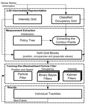
The system processing flow can be decomposed into tree main stages: Intermediate Representation, Measurement Extraction and Tracking (see Fig.1).

Figure 1. System Overview.

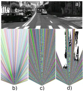
The Intermediate Representation module consists in mapping the 3D dense information into two 2.5D grid-based representations: Occupancy Grid and Intensity Grid. Both maps have the same size and resolution and can be regarded as a projection of the 3D data into a more compact bird-eye view space. The raw occupancy grid cells are computed by processing a stereovision-based elevation map (see Fig. 2) in which each cell stores the information of its height and type (road, object or traffic isle) [8]. In the case of the Intensity Grid, the cell values are estimated as the average intensity of its associated 3D points.

The Measurement Extraction module uses the two grid maps to extract a set of rectangular NxN blocks. In the initialization step we pre-compute a Policy Tree. The Policy Tree is used to store all possible paths between the ego-vehicle’s position and the most visible object points, through the grid. The block entities are extracted by exploring the Policy Tree with a depth-first-search technique.

Figure 2. Intermediate Representations. a) An image from the traffic scene. b) The grayscale intensity grid c) The classified occupancy grid. The grid cells are labeled as Object (red), Road (blue) and Traffic Isle (yellow).

Figure 3. Generating the Policy Tree. Top: a simple scenario containing only three rays. The grid points that are processed more than once by deiferent rays maintain a single copy in the tree. The cell colors show how they are assigned to the tree branches. Bottom: the resulted structure.

In the Tracking stage we estimate the optimal state parameters for each individual grid block using a Rao-Blackwellized Particle Filter. The position and speed parameters are estimated by a weighting-resampling mechanism, the occupancy values are updated by using binary Bayes filters while the intensity values are updated by using individual Kalman Filters for each block cell. The representation and tracking modules will be described in detail in the next sections.

III. EXTRACTING GRID BLOCKS BY USING POLICY TREES The purpose of this stage is to extract a set of the most visible (not occluded) rectangular patches – grid blocks. Each block can be regarded as a 2D surface patch that is centered into an object contour point, and includes the information about the object position, occupancy and intensity component. The extracted blocks are used as the measurement information for the subsequent tracking algorithm. Thus, instead of performing the data association and filtering at the object level we split the object model into smaller entities, each entity being tracked separately.

A. Extracting Object Contours by using Policy Trees

In our previous work [16] we introduced the

BorderScanner algorithm for extracting object contours,

Figure 4. Object delimiters extraction by exploring Policy Trees. a) An image from the traffic scene. b) A Policy Tree constructed at a lower resolution. For a better visibility each tree branch has a diferent color. c) A Policy Tree covering the entire grid space. Each grid cell is assigned to a tree node. d) The result of exploring the occupancy grid via traversing the tree structure. Black values denote occupied cells. The occupancy grid corresponds to the traffic scene (a).

also referred to as “object delimiters”. The main idea of the algorithm is to extract a contour C_m ={c₁,...,c_NC} for each object by accumulating the most visible grid cells c_i that are occupied. This is achieved by generating a virtual ray which extends from the ego-vehicle position and traverses the occupancy grid in a radial direction with fixed increments. At each step, the closest occupied point along the virtual ray is accumulated into the contour list Cm. The first observation is that in order to cover the entire space it is necessary to scan the grid surface at a high resolution. Moreover, the scanning axes and the position of the candidate object cells along these axes are re-computed at each frame. The second observation is that, at high scanning resolutions, the occupancy gird cells that are close to the origin position are likely to be traversed more than once. To minimize the algorithm complexity and to solve the overlapping sub-problems we introduced a Policy Tree, which is regarded as a predefined path structure that is used to explore the occupancy grid space. The object delimiter extraction algorithm is described by the two main phases:

1) Policy Tree Creation: The idea of creating path search data structures is widely used in the context of navigation or path planning applications [18][19]. In our case we construct a specific tree-based structure T that stores all possible paths starting from the point of origin (the camera position). A node si in the tree T can be described as a policy s(ci) that determines the search position of the next grid cell cj given the position of the current cell ci:

] .. 1 [ ], .. 1 [ ),

(c i NG j NG

s

cj = i ∈ ∈ (1)

ALGORITHM I CREATING THE POLICY TREE

1: s0

←

α

3: sgoal

←

α

←

5: while _(sc

_≠

6: //Bresenham Algorithm[20] 7: sc

←

α

α

9: //keep a single copy of sc 10: move scnode from

α

α

where NG represents the grid size. Therefore, every node si in the tree is associated to a grid cell ci and also contains a reference to the next node. The root of the tree s0 stores the position of the observation point, while the tree leafs

correspond to the grid boundary cells. The grid points that are processed more than once maintain a single copy in the tree (see Fig. 3). As the search space has the same size and the same resolution in all frames, the Policy Map is constructed only once, in the initialization step (Algorithm I). The generated structure can also be stored as a map of linked lists, each list denoting a tree branch.

2) Exploration: The exploration step is performed at each frame by using the generated Policy Tree. The purpose of this step is to find all closest object points that are occupied (see Fig. 4). In order to accumulate the cells of interest we use a depth-first search strategy starting from the root of the tree and traversing as far as possible along each branch until an occupied cell is discovered. All the object points that are found are accumulated into a contour list: Cm ={c1,...,cNC}_.

B. Grid Block Entities

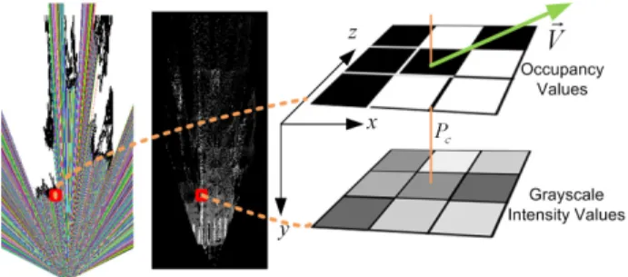
Each accumulated cell in the contour list C_m is used as a seed point for constructing a so called “grid block”. The idea is to compute a set of independent medium level entities incorporating the information about the object position, color and geometry (see Fig. 5). For each selected contour point we define a window of NxN cells, centered in the point’s position. Then we use the defined window to extract a vector of NxN occupancy values from the occupancy grid and a vector of NxN grayscale values from the intensity grid. Therefore, a grid block model is described by the following parameters:

Figure 5. Grid Block model. Left: the Occupancy Grid with the extracted delimiters. Middle: The Intensity Grid. Right: the three components defining the estimated state: position, occupancies and grayscale values.

• The dynamic component T z x v

v z x

S =[ , , , ] being described by the position P_c(x,z) and speed parameters

) , (vx vz

V

r

. The block position is given by the position of its center point P_c(x,z) in the car coordinate system.

• The geometry component, which is described by a set of occupancy values O={o₁,o₂,...,o_K}, where K represents the number of neighbor cells included in a NxN window.

• The intensity component specifying a vector of grayscale intensity values G={g1,g2,...,gK}. Both sets Gand O have the same size K =N⋅N.

Therefore, we can describe the appearance part of each block as a collection of cells {bi(oi,gi)|i=[1..K]}, where each cell is defined by a pair of occupancy oi and grayscale

gi terms. Considering the parameters described above, at time t the overall grid block state is defined as:

T K K

z x

t x z v v o o o g g g

X =[ , , , , ₁, ₂,..., , ₁, ₂,..., ] (2)

and can be written in a more compact form as: T

t S O G

X =[ , , ] (3)

IV. GRID BLOCK TRACKING

The purpose of the tracking mechanism is to estimate the optimal state X_t of each individual block entity. The problem can be formulated as a Bayes filter, which aim to recursively update the posterior probability distribution

) ... , |

(Xt Z1 Z2 Zt

p given all noisy measurements

} ..., , { 1 2 :

1t Z Z Zt

Z = up to the present time t. Typically, particle-based filtering techniques [21] are used as an effective means to work with multi-modal distributions. However, a disadvantage in the case of particle filtering algorithms is that they are not suitable for high-dimensional state spaces, where the complexity tends to grow exponentially with the number of state parameters. To keep a low computational complexity we adopt a Rao-Blackellized Particle Filter [22]. Therefore, we apply the “Rao-Blackwellization” process to estimate a part of the object state analytically by factorizing the posterior distributionp(Xt |Z1t:)as follows:

) , | , ( ) | ( ) |

(Xt Z1:t p St Z1:t p Ot Gt St Z1:t

p = (4)

The first termp(St |Z1t:)describes the grid block position and speed posterior probability and is approximated by a set of weighted particles:

]} .. 1 [ , , { ) |

(S Z1: S w i N

p i

t i t t

t ≈ = (5)

Each particle i t

S represents a hypothesis for the position and velocity of a given block entity.

The second factor p(Ot,Gt|St,Z1t:)describes the block appearance posterior probability conditioned on its motionS_t. We consider that the occupancyO_tand intensityG_tcomponents are conditionally independent given

t

S andZ_1:t:

) , | ( ) , | ( ) , | ,

(Ot Gt St Z1:t p Ot St Z1:t p Gt St Z1:t

p = (6)

The occupancy term p(O_t|S_t,Z_1t:) is recursively updated using a binary Bayes filter for each individual block cell. The intensity factor p(G_t|S_t,Z_1t:) is estimated with

1D Kalman Filters (one per block cell). The sample state can be defined now as:

]} .. 1 [ , ] , , , [ |

{q q S w O Gti T i N

i t i t i t i t i

t = = (7)

Next, we will describe the main steps of the proposed tracking solution.

A. Initialization

The initialization step generates an initial prior probability p(X0) for each newly detected target. This is achieved by drawing a set of random hypotheses around each unassociated block measurement:

]} .. 1 [ , ] , , , [ | { )

(X0 q0 q0 S0 w0 O0 G0 i N

p ≈ i i = i i i i T = (8)

The object occupancy i

O0 and intensity i

G0components are initialized with the corresponding observation values.

B. State Prediction

The aim of this step is to predict the current state X_t

given the previous informationX_t−1and the motion model )

| (Xt Xt−1

p . Each particle is moved based on its state transition probability. Additionally, each hypothesis state is altered according to a random noise. Before applying the prediction step we must also consider the ego-car motion information. As the ego-vehicle parameters are provided through the CAN bus, we use this information to modify the position of each particle. The position and

speed T

t z t x t t

t x z v v

S =[ , , _,, _, ] of each hypothesis is predicted given its previous state S_t−1 according to the same linear motion model previously described in [15]:

C. Measurement Update

The purpose of the measurement update step is to assign importance weights to the predicted particles according to how well these hypotheses match the measurement data.

) |

( i

t t t X q

Z

p = (9)

Additionally, each particle’s occupancy and intensity parameters are updated analytically. The occupancy values are estimated by using binary Bayes filters while the gray intensities are updated by means of Kalman filters. For our tracking solution we assume that the measurement data is given as a list of blocks extracted from the two grid-based representations (occupancy grid and intensity grid). (see Fig. 6). For each block, the measurement vector is defined by three main components:

T g t o t p t t Z Z Z

Z =[ , , ] (10)

where p t

Z describes the measurement grid block positions,

o t

Z denotes the observed occupancy values and g t

Z

represent the measured intensity component. We can express the measurement model as:

Figure 6. From the raw measurements to the grid blocks. a) Left camera image b) The Intensity Grid c) The detected block entities with assigned gray values extracted from the Intensity Grid (b). d) The raw occupancy values. Black means occupied. e) The computed occupancy probabilities according to the used Forward Probability Model. White colors indicate occupied cells. f) The same block entities as in (c) represented by occupancies from (e). Even the extracted measurement block entities in (c) and (f) are visually grouped into continuous object delimiters, they are tracked individually.

) | , , ( ) |

( t

g t o t p t t

t X p Z Z Z X

Z

p = (11)

By assuming that all measurement components are independent we obtain:

) | ( ) | ( ) | ( ) |

( g _t

t t o t t p t t

t X p Z X p Z X p Z X

Z

p = (12)

Therefore, we estimate the particle weights by considering the three terms provided by the equation (12).

1) Computing the Stereovision Uncertainties

In order to take into account the noises provided by the stereovision system, the uncertainty model should be defined. By using an error model similar to one described in [23], we approximate the longitudinal error σ_zand the lateral σ_xerror as:

z x f

b

z z

x d z

⋅ = ⋅

⋅

= σ σ σ

σ ,

2

(13)

where b is the distance between the two cameras (baseline),

f is the focal distance , x and z are the coordinates of a point in 3D and σ_d represents the disparity error in pixels. The error standard deviations are estimated for all grid cells and are stored into a look-up table.

2) Defining the Inverse Sensor Model

In order to update the occupancy probability of each block cell p(ok)we require an inverse sensor model

) |

( S

t

xz Z

c

p , where c_xzis a new occupancy probability stored at the position (x,z) in the grid and S

t

Z represents the stereo measurements. As the raw observations (see Fig. 6.d)

are affected by the stereo uncertainties we consider that each grid cell is described by a probability distribution with the standard deviations defined in the previous step. We are interested to determine the occupancy value of a certain cell

xz

c given also the probabilities of its neighbor measurements. As in the Kernel Density Estimation approaches that use Parzen windows [24] we estimate the occupancy of a cell c_xz by placing a window of size

x

σ

2 x2σ_zat the position of c_xz and then, determine, for all occupied neighbor cells that fall within the window, what is the contribution of each observation c_ij to the cell c_xz. The occupancy values c_xz are approximated as (see Fig.6.e):

        − + − − + = − = + = − =

∑ ∑

= x z

z z x x i z j x z i z i x j x

j x z

S t

xz Z e

c

p σ σ

σ

σ σ

σ πσ σ

ϖ

2

2 _{( )}

) ( 2 1 2 1 1 ) |

( (14)

where

ϖ

3) Particle Weighting

Having the measurement information given as a list of extracted blocks Zt ={Zt,1,Zt,2,...,Zt,N}, for each particle

i t

q its weight i

w is determined as follows:

a) Position weights: for the position component we compute a distance between the particle and the closest corresponding measurement blockZ_t,k:

) , ( min ) , ( , } .. 1

{ tm

i t N m t i

t Z d q Z

q d

∈

= (15)

The distance to the closest measurement ( , t) i t Z

q

d can

be decomposed into two x and z components (dx, dz) where

2 2

) ,

(q Z dx dz

d t i

t = + . It must be noted that, the

particle-to-measurement associations are determined by using a pre-computed distance transform map where each cell in the map stores the information regarding the closest measurement block. Therefore, for each hypothesis, the corresponding measurement is found in O(1) by superimposing the particle model on the distance map. The weight received by the particle position i

p

w is estimated by converting the distance metric according to:

        + − = = = 2 2 2 2 2 1 2 1 ) |

( x z

dz dx z x i t g t i

p p Z X q e

w σ σ

σ πσ

(16)

b) Occupancy weights: for the occupancy component we define a dissimilarity metric ( , o_, )

m t i

t Z

q

d by calculating the normalized sum of absolute differences between corresponding occupancy elements in the particle o_ki and the measurement cells m

k o . K o p o p Z q d m k i k o m t i

t, ) ( ) ( )/

( _, = − (17)

where i is the particle index, m represents the measurement block index, p(ok) denotes the occupancy probability of a cell o_k, k is the index of the occupancy element k∈[1..K], and K represents the total number of occupancy values in a given particle or measurement block. The resulted heuristic metric is used to estimate the occupancy weight:

        − = =

= ₂ ,

2 ) , ( 2 1 exp 2 1 ) | ( o o m t i t o i t o t i o Z q d q X Z p w σ πσ (18)

c) Intensity weights: the same strategy is applied for the particle gray values. The difference here is that we are taking into account only the intensity of occupied cells (belonging to obstacles). The gray dissimilarity measure is defined as:

) /(

) ,

( , g occ

m k i k g m t i

t Z g g N N

q

d = − ⋅ (19)

where Ngrepresents the number of possible gray intensities and Nocc is the number of cells that are occupied in both particle and measurement block. The intensity weight is computed according to:

        − = =

= ₂ ,

2 ) , ( 2 1 exp 2 1 ) | ( g g m t i t g i t g t i g Z q d q X Z p w σ πσ (20)

As described in the equation (12), the overall particle weight

w

i g i o i p i w w w

w = ⋅ ⋅ (21)

4) Updating the Occupancy Component

This step updates the occupancy component }

,..., , { 1 2

i K i i i

t o o o

O = for each hypothesis i

t

q . The update method relies on the inverse sensor model p(cxz |ZtS) previously described in the step 2. The computed values are assigned to the extracted block measurements so that:

) | ( ) | ( S t xz S t m

k Z p c Z

o

p = (22)

where k is the index of the occupancy element k∈[1..K], m

represents the index of the measurement block, and cxz is the corresponding grid cell. Assuming that the occupancy of individual cells is independent we can decompose the update problem into many binary estimation subproblems. The new measurements can be recursively incorporated for each individual cell by using a binary Bayes filter. As described in [17], this can be expressed in the log-odds representation as: ) ( ) ( 1 log ) | ( 1 ) | ( log , 1 , m k m k S t m k S t m k i k t i k t o p o p Z o p Z o p l

l + −

− +

= ₋ (23)

where i k t

l, represents the log-odds ratio defined according to:

) | ( 1 ) | ( log : 1 : 1 , S t i k S t i k i k t Z o p Z o p l − = (24)

The term i k t

l−1, denotes the previous log-odds value. The second term in the equation (23) describes the inverse sensor model while de last term represents the prior log-odds ratio. The new occupancy probability of a given element i

k

o in the particle i t

q can be estimated according to: )

) 1 ( 1 ( ) |

( 1

: 1

, −

+ −

= ltik

S t i

k Z e

o

p (25)

.5) Updating the Particle’s Intensity Values

This step updates the particle grayscale component }

,..., , { 1 2

i K i i i

t g g g

G = with the new measurements. For each grayscale element we use a 1D Kalman filter to estimate its new mean and variance (ˆi, _g)

k

g σ . The new measurements )

,

( m

m k

g σ are incorporated according to:

1

2 2 2 2 2

2 2

1 1 ,

ˆ

−

    

  

+ = +

+ =

m g g m g

m k g i k m i k

g g g

σ σ σ σ σ

σ σ

(26)

The two variances are tuned experimentally.

D. State Estimation

As the result of measurement update step we have determined the new weights of the particle population and estimated the belief of each particle about its occupancy and grayscale intensity. The current posterior density can be estimated now as:

i t N

i i tX

w X

∑

=

=

1

)

(27)

E. Resampling and Merging

The resampling stage consists in drawing from the previous sample distribution according to a probability proportional to the particle weights. As the result, the particles with high weights are multiplied by replacing the particles with low weights. Also, at this stage we decide whether the similar trackers should be merged. For merging the particle distributions we use a separate map to accumulate all overlapping candidates. When a new block state is estimated, its position is registered into the overlapping map. In the resampling step, we test if in the same estimated grid position there is another tracklet. The candidates having the similar speed vectors are subjected to the merging process. As all tracklets share the same measurement space we use all particles of the selected candidates to estimate the new state. The new population of particles will be drawn by sampling from all candidate distributions.

V. EXPERIMENTAL RESULTS

The proposed method has been tested on various traffic scenarios in Cluj-Napoca, Romania. For our tests we have used a 2.66GHz Intel Core 2 Duo Computer with 2GB of RAM. Both input grids (occupancy and intensity grid) have the same size of 240 rows x500 columns (0.1 m x 0.1 m

Figure 7. Modeling and Tracking results. a) An image from the traffic scene. b) The corresponding population of particles projected into the grid space (top view). Each particle is represented as a point. High intensities indicate high weights. c) The estimated grid blocks described by their occupancy values and the assigned speed vectors. d) The result projected in the image space. Each red segment corresponds to an extracted measurement and has the same height as the associated object. e) A traffic scenario including a partially visible car.

cells). Some qualitative results including intermediate processing steps are presented in the Fig. 7. Fig. 7.b shows how the entire population of particles is projected in the grid space (top view). Each particle is represented as a point. The particles are weighted based on how well they match the new observations. High intensities indicate high weights. Fig. 7.c illustrates the estimated grid blocks and the assigned speed vectors. Fig. 7.d shows how the resulted dynamic environment representation is projected in the image space. Each red segment corresponds to an extracted measurement and has the same height as the associated object. Another traffic scenario including partial visible obstacles is shown in Fig. 7.e. We have compared the performance of the proposed Policy Tree based delimiter extraction solution with a previously developed BorderScanner method [16] in terms of the execution time. Besides the space size, the Border Scanner approach complexity depends also on the radial step size. For example, with a radial step of 0.01 radians the average processing time is about 5ms, however when covering the entire 240x500 grid space, the running time increases at 22.8 ms. In comparison with the BorderScanner method, the Policy Tree based approach reduces the delimiter extraction time to 3.63ms / frame. Fig. 8 presents a comparison between the proposed tracking solution (RBPF-

TABLEI SPEED ESTIMATION ACCURACY

Accuracy Metric GRID-BLOCKS ICP-KALMAN [25]

Figure 8. Comparison between the proposed Grid Block representation and tracking approach and the existing ICP-KALMAN method [25].

Grid-Blocks) and an existing ICP-based object tracking approach (ICP-KALMAN) [25]. The test implies a test vehicle passing from right to left, being in the field of view for 26 frames. The ground truth speed is provided by a high accuracy GNSS device, mounted on the test vehicle. The target car velocity was estimated as the average speed of its associated block entities. The mean absolute error of the speed estimation was 2.97 km/h for the proposed method and 3.7 km/h for the ICP-KALMAN solution [25]. In the case of urban traffic experiments, the average number of tracked grid blocks was 486. For each block we set a fixed size of 3x3 cells and a fixed number of 40 particles. The average processing time of the proposed tracking solution was about 194ms.

VI. CONCLUSIONS

In this paper we presented a new stereovision based method for modeling and tracking crowded traffic scenes. The method uses two grid-based representations, namely an intensity grid and a classified occupancy grid. In order to accelerate the measurement extraction process and to avoid the overlapping subproblems, a Policy Tree is employed. The measurements are given in form of rectangular grid blocks, comprising a dynamic part, a geometry part and an intensity part. The proposed medium level tracking solution is based on a Rao-Blackwellized particle filter able to process high dimensional state spaces. This allows handling the data association at particle level in a natural manner. The proposed method is also able to deal with the uncertainties of the stereovision system and to incorporate the intensity information into the estimated state. As future work, it would be important to extend the tracked state with the height information. The system processing time can also be improved by further optimizations.

REFERENCES

[1] S. Sivaraman, M. M. Trivedi, "Looking at Vehicles on the Road: A Survey of Vision-Based Vehicle Detection, Tracking, and Behavior Analysis", IEEE Trans. onIntell. Transp. Syst., vol.14, no.4, pp.1773-1795, Dec. 2013.

[2] A. Broggi, S. Cattani, M. Patander, M. Sabbatelli and P. Zani, "A full-3D voxel-based dynamic obstacle detection for urban scenario using stereo vision", in Proc. of IEEE ITSC 2013, pp.71-76, 6-9 Oct. 2013.

[3] U. Franke, C. Rabe, H. Badino, and S. Gehrig, “6d-vision: Fusion of stereo and motion for robust environment perception,” in DAGM ’05, 2005, pp. 216-223.

[4] R. Danescu, F. Oniga, S. Nedevschi, "Modeling and Tracking the Driving Environment With a Particle-Based Occupancy Grid," IEEE Trans. on Intell. Transp. Syst., vol.12, no. 4, pp.1331-1342, Dec. 2011. [5] M. Perrollaz, J.-D. Yoder, A. Nègre, A. Spalanzani, and C. Laugier, "A

visibility-based approach for occupancy grid computation in disparity space", IEEE Transactions on Intelligent Transportation Systems, vol. 13, no. 3, pp. 1383–1393, Sep. 2012.

[6] Thien-Nghia Nguyen, B. Michaelis, A. Al-Hamadi, M. Tornow, M. Meinecke, "Stereo-Camera-Based Urban Environment Perception Using Occupancy Grid and Object Tracking", in IEEE Transactions on Intelligent Transportation Systems, vol.13, no.1, pp.154-165, 2012 [7] D. Pfeiffer and U. Franke, "Modeling Dynamic 3D Environments by

Means of The Stixel World," IEEE Intelligent Transportation Systems Magazine, vol.3, no.3, pp.24,36, 2011.

[8] F. Oniga and S. Nedevschi, “Processing Dense Stereo Data Using Elevation Maps: Road Surface, Traffic Isle, and Obstacle Detection”, IEEE Transactions on Vehicular Technology, vol. 59, vo. 3, March 2010, pp. 1172-1182.

[9] M.A.Garcia and A.Solanas, "3D Simultaneous Localization and Modeling from Stereo Vision", in Proc. of IEEE ICRA, New Orleans, USA, April-May 2004, 847-853, ISBN: 0-7803-8233-1.

[10] S. Vedula, S. Baker, P. Rander, R. T. Collins, T. Kanade, “Three-Dimensional Scene Flow”, IEEE Trans. Pattern Anal. Mach. Intell. 27(3): 475-480 (2005)

[11] R. Danescu, S. Nedevschi, “A Particle-Based Solution for Modeling and Tracking Dynamic Digital Elevation Maps”, IEEE Transactions on Intelligent Transportation Systems, vol.15, no.3, pp.1002-1015, June 2014.

[12] J. Aue, M.R. Schmid, T. Graf, J. Effertz, "Improved object tracking from detailed shape estimation using object local grid maps with stereo", in Proc. of ITSC 2013, pp.330,335, 6-9 Oct. 2013

[13] M. Schutz, N. Appenrodt, J. Dickmann, K. Dietmayer, "Simultaneous tracking and shape estimation with laser scanners", in Proc. of 2013 16th International Conference on Information Fusion (FUSION), pp.885,891, 9-12 July 2013

[14] P. Steinemann, J. Klappstein, J. Dickmann, F. von Hundelshausen, and H. Wunsche, "Geometric-Model-Free Tracking of Extended Targets Using 3D-LIDAR-Measurements", in Proc. of SPIE, Vol. 8379, pp. 83790C-83790C-12, 2012.

[15] A. Vatavu, R. Danescu, and S. Nedevschi, "Tracking multiple objects in traffic scenarios using free-form obstacle delimiters and particle filters", in Proc. of. ITSC 2013, pp.1346,1351, 6-9 Oct. 2013

[16] A. Vatavu, S. Nedevschi, and F. Oniga, “Real Time Object Delimiters Extraction for Environment Representation in Driving Scenarios”, In Proc. of ICINCO-RA 2009, Milano, Italy, 2009, pp 86-93.

[17] S. Thrun, W. Burgard, and D. Fox, "Probabilistic robotics", in MIT press, 2005.

[18] C. Fulgenzi, A. Spalanzani, C. Laugier, "Probabilistic motion planning among moving obstacles following typical motion patterns," in Proc of IROS 2009, pp.4027-4033, 10-15 Oct. 2009

[19] E. Lu, W.-C. Lee, and V. Tseng, "Mining fastest path from trajectories with multiple destinations in road networks", Knowledge and Information Systems, pp. 1–29

[20] J. E. Bresenham, "Algorithm for Computer Control of a Digital Plotter", IBM Systems Journal 4, No.1, 25-30, 1965.

[21] M. Isard and A. Blake. Condensation, “Conditional density propagation for visual tracking”, in International Journal of Computer Vision, 29(1):5–28, 1998.

[22] A. Doucet, N. De Freitas, K. Murphy, S. Russell, "Rao–Blackwellised particle filtering for dynamic Bayesian networks" in Proc. of the Sixteenth conference on Uncertainty in artificial intelligence, 2000, pp. 176–183.

[23] Gallup, D.; Frahm, J.-M.; Mordohai, P.; Pollefeys, M., "Variable baseline/resolution stereo," in Proc. of CVPR 2008, pp.1-8, 23-28, 2008 [24] E. Parzen, "On Estimation of a Probability Density Function and Mode",

The Annals of Mathematical Statistics 33, no. 3, pp 1065--1076, 1962 [25] A. Vatavu, S. Nedevschi, "Modeling Unstructured Environments with

Dynamic Persistence Grids and Object Delimiters in Urban Traffic Scenarios", in Proc. of IV 2013, Gold Coast, Australia, 23-26 June, 2013, pp. 505 – 510.