The Approximate Solution for Solving Linear Volterra Weakly Singular Integro-Differential Equations by Using Chebyshev Polynomials of the First Kind

AUSTRALIAN JOURNAL OF BASIC AND

APPLIED SCIENCES

-ISSN:1991

Journal home page: www.ajbasweb.com

Open Access Journal

Published BY AENSI Publication

© 2017 AENSI Publisher All rights reserved

This work is licensed under the Creative Commons Attribution International License (CC BY).

http://creativecommons.org/licenses/by/4.0/

ToCite ThisArticle:Dr.Eman Ali, Dr.Nabaa Najdi, Wafaa Abd &Wafaa faeik keidan., The Approximate Solution for Solving Linear Volterra Weakly Singular Integro-Differential Equations by Using Chebyshev Polynomials of the First Kind. Aust. J. Basic & Appl. Sci.,

11(7): 102-109, 2017

The Approximate Solution for Solving Linear Volterra Weakly Singular

Integro-Differential Equations by Using Chebyshev Polynomials of the

First Kind

1_{Dr.Eman Ali,} 2_{Dr.Nabaa Najdi,} 3_{Wafaa Abd and} 4_{Wafaa faeik keidan}

. , Iraq Diyala College of Science, Department of Mathematics, University,

Diyala

1,2,3,4

Address For Correspondence:

Dr.Eman Ali, Diyala University, College of Science, Department of Mathematics, Diyala, Iraq.

A R T I C L E I N F O A B S T R A C T Article history:

Received 18 February 2017 Accepted 5 May 2017

Available online 10 May 2017

Keywords:

Chebyshev polynomials, Integro-differential equations, Linear Volterra, Trapezodial rule, Weakly singular kernel.

In this paper, we use Chebyshev polynomials method of the first kindof degree n to solve linear Volterra weakly singular integro- differential equations (LVWSIDEs) of the second kind. This techniques transform the linear Volterra weakly singular integro-differential equations to a system of a linear algebraic equations. This application was presented to illustrate the efficiency and accuracy of this method.

INTRODUCTION

Volterraweaklysingular integro-differential equations is used. application is given in section 4 for confirming the efficiency of the proposed method .Section 5 contains conclusions of the paper.

2.Chebyshev Polynomials Of the First Kind 𝑻𝒏(𝒙), (Mason, Handscomb, 2003):

The Chebyshev Polynomials of the first kind of degree n is as set of orthogonal polynomials and it is defined by the recurrence relation

𝑇0(𝑥) = 1

𝑇1(𝑥) = 𝑥

𝑇𝑛+1(𝑥) = 2𝑥𝑇𝑛(𝑥) − 𝑇𝑛−1(𝑥), for each 𝑛 ≥ 1. (1)

2.1 Properties of Chebyshev Polynomials 𝑻𝒏(𝒙):

1. The Chebyshev Polynomials of the first kind 𝑇𝑛(𝑥), 𝑛 = 0,1, … are aset of orthogonal polynomials over

the interval [-1,1] with respect to the weight function𝑤(𝑥) = (1 − 𝑥2₎−1 2⁄ _{, that is:}

∫ 𝑤(𝑥)𝑇𝑛(𝑥)𝑇𝑚(𝑥)𝑑𝑥 = {

0 𝑛 ≠ 𝑚 𝜋

2 𝑛 = 𝑚 ≠ 0

𝜋 𝑛 = 𝑚 = 0 1

−1 (2)

2. The Chebyshev polynomials of the first kind can be defined by the trigonometric identity 𝑇𝑛(cos(𝜃)) =

cos (𝑛𝜃) for n=0,1,2,3,…

3.𝑇𝑛(𝑥) has n distinct real roots 𝑥𝑖 on the interval [-1,1], these roots are defined by :

𝑥𝑖= cos (

(2𝑖+1)𝜋

2𝑁 ) , 𝑖 = 0,1,2, … . , 𝑁 − 1 (3)

are called Chebyshev nodes.𝑇𝑛(𝑥) assumes its absolute extrema at

𝑥𝑗= cos (

𝑗𝜋

𝑁) for j=0,1,2,…,N (4)

3. A polynomial of degree N in Chebyshev form is a polynomial

𝑝(𝑥) = ∑𝑁𝑛=0𝑎𝑛𝑇𝑛(𝑥) (5)

Where 𝑇𝑛 is the 𝑛𝑡ℎ Chebyshev form

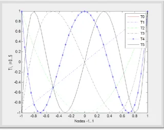
The first few Chebyshev polynomials of the first kind for N=0,1,2,3,4,5 are given in figure(1)

Fig. 1:The first few Chebyshev polynomials of the first kind for N=0,1,2,3,4,5.

2.2 Shifted Chebyshev Polynomials:

Shifted Chebyshev polynomials are also of interest when the range of the independent variable is [0,1] instead of [-1,1].The shifted Chebyshev polynomials of the first kind are defined as

𝑇𝑛∗(𝑥) = 𝑇𝑛(2𝑥 − 1), 0 ≤ 𝑥 ≤ 1 (6)

Similarly, one can also build shifted polynomials for a generic interval [a,b] where

𝑥̃𝑖= 𝑏−𝑎

2 𝑥̅𝑖+

𝑏+𝑎

The first few Chebyshev polynomials of the first kind for N=0,1,2,3,4,5 for interval [0,1] are given in figure(2).

Fig. 2:The first few shifted Chebyshev polynomials of the first kind for N=0,1,2,3,4,5.

3. The Approximate Solution Of Linear Volterra Weakly Singular Integro-Differential Equations: We consider the first-order LVWSIDEs of the following form:

𝑝(𝑥)𝑦′_{(𝑥) − 𝑦(𝑥) − ∫ 𝑘(𝑥, 𝑡)𝑦(𝑡)𝑑𝑡 = 𝑓(𝑥) 𝑥 ∈ [𝑎, 𝑏]}𝑥

𝑎 (8)

with initial condition 𝑦(𝑎) = 𝛽 where 𝛽is a constant and 𝑘 and 𝑓 are given functions and 𝑦 is the solution

to be determined .Moreover we assume that the kernel 𝑘(𝑥, 𝑡) =𝐻(𝑥,𝑡)

|𝑥−𝑡|𝛼 ∀ 𝑥, 𝑡 ∈ [𝑎, 𝑏]where 0 < 𝛼 < 1.As well

as we assume that the kernel 𝐻 is in 𝐿2[𝑎, 𝑏] and the unknown 𝑦 and the right hand side 𝑓 are in 𝐿2[𝑎, 𝑏].Also

we suppose that 𝑦(𝑥) satisfies in the Lipschitz condition with respect to x,

|𝑦(𝑥1) − 𝑦(𝑥2)| ≤ 𝐿𝑥|𝑥1− 𝑥2| (9)

to determine an approximate solution of (8).Firstly if the function 𝑦(𝑥)defined in [−1,1].We suppose this function may be represented by first kind CPs(Qinghua, 2014):

𝑦(𝑥̅) ≅ ∑∞𝑖=0𝑇𝑖(𝑥̅)𝑏𝑖 (10)

If we truncated the series (4.3), then we can write (4.3) as follows:

𝑦(𝑥̅) ≅ ∑𝑁𝑖=0𝑇𝑖(𝑥̅)𝑏𝑖≅ 𝑇(𝑥̅)𝐵 (11)

𝑦′(𝑥̅) ≅ (∑𝑁𝑖=0𝑇𝑖(𝑥̅)𝑏𝑖) ′

≅ (𝑇(𝑥̅)𝐵)′ (12)

where 𝑇(𝑥̅) = [𝑇0(𝑥̅), 𝑇1(𝑥̅), 𝑇2(𝑥̅), … , 𝑇𝑁(𝑥̅)], 𝐵 = [𝑏0, 𝑏1, 𝑏2, … , 𝑏𝑁]𝑇

clearly T is 1 × (𝑁 + 1) vectors and B is (𝑁 + 1) × 1 vectors.then the aim is to find chebyshev coefficients, that is the matrix B. we first substitute the chebyshev nodes, which are defined by:

𝑥̅𝑖= cos (

(2𝑖+1)𝜋

2𝑁 ) , 𝑖 = 0,1,2, … , 𝑁 − 1into (11) and (12) and then rearrange anew matrix form to

determine B:

𝑝𝑦′_{− 𝑦 − 𝑘 = 𝑓 (13)}

In which 𝑘is the linear integral part of (8) and

𝑝𝑦′₌

(

𝑝(𝑥̅0)𝑦′(𝑥̅0) 𝑝(𝑥̅1)𝑦′(𝑥̅1)

. . .

𝑝(𝑥̅𝑁)𝑦′(𝑥̅𝑁)) , 𝑦 =

( 𝑦(𝑥̅0) 𝑦(𝑥̅1)

. . .

𝑦(𝑥̅𝑁))

, 𝑓 =

( 𝑓(𝑥̅0) 𝑓(𝑥̅1)

. . .

𝑓(𝑥̅𝑁))

, 𝑘 =

( 𝑘(𝑥̅0) 𝑘(𝑥̅1)

. . .

𝑘(𝑥̅𝑁))

by substituting(11) and(12) into (13) gives linear algebraicequations in (𝑁 + 1) unknown coefficients .These equations are solved by using (Matlab R2010b) to obtain the unknown coefficients 𝐵which are then substitute into (11) to get the approximate solution of (8).Or if the function 𝑦(𝑥)defined in [0,1]. We use shifted CPsby using the transformation 𝑥̃ =1

2[(𝑏 − 𝑎)𝑥̅ + (𝑎 + 𝑏)] transforms the nodes𝑥̅𝑖in [−1,1]into the

corresponding nodes 𝑥̃𝑖 in[0,1].

3.1 The Algorithm for solving (LVWSIDEs) into [-1,1]: Input : 𝑎, 𝑏, 𝛼, 𝑁, 𝑀, 𝑦(𝑥), 𝑓(𝑥), 𝑝(𝑥), 𝜖.

Output : The approximate solution of the LVWSIDEs. Step 1: process: Find 𝑇𝑖(𝑥̅), (𝑇𝑖(𝑥̅))′. (CPs)

Step 2: Find roots 𝑥̅𝑖, 𝑖 = 0,1, … , 𝑁. (roots of CPs)

Step 3: Find roots

𝑡𝑖𝑗 = 𝑎 + 𝑗 + 𝑘𝑖± 𝜖, 𝑘𝑖=

𝑥̅𝑖− 𝑎

𝑀 , 𝑖 = 0,1, … , 𝑁, 𝑗 = 0,1, … , 𝑀, 𝑥̅ = 𝑡.

Step 4: Calculate 𝑅𝑖=

𝑘_𝑖

2[𝑌𝑖0+ 2 ∑ 𝑌𝑖𝑘+ 𝑌𝑖𝑀]

𝑀−1

𝑘=1 (Trapezoidal rule)Where 𝑌𝑖𝑗 =

𝑡𝑖𝑗(𝑡)

|𝑥̅_𝑖−𝑡_𝑖𝑗|𝛼 , 𝑖 = 0,1, … , 𝑁, 𝑗 = 0,1, … , 𝑀.

Step 5: Construct the system:

𝐴𝑖𝑘= 𝑏𝑘∗ (𝑝(𝑥̅𝑖) ∗ (𝑇𝑘(𝑥̅𝑖))

′

− 𝑇𝑘(𝑥̅𝑖)) − 𝑏𝑘∗ 𝑅𝑖, 𝑖, 𝑘 = 0,1, … , 𝑁,

(where 𝑏𝑘 are unknown values),𝐵𝑖= 𝑓(𝑥̅𝑖), 𝑖 = 0,1, … , 𝑁.

Step 6: solve the linear system 𝐴𝑖𝑘= 𝐵𝑖 by using 𝑋𝑖= 𝑖𝑛𝑣(𝐴𝑖𝑘) ∗ (𝐵𝑖)𝑡and find the unknowns 𝑏𝑘.

Step 7: Calculate the approximate function 𝑦𝑁(𝑥̅) = ∑𝑁𝑖=0𝑇𝑖(𝑥̅)𝑏𝑖

Step 8: Calculate absolute error is the comparison between the exact and the approximate solutions.

Step 9: END of the process.

3.2 The Algorithm for solving (LVWSIDEs) into [0,1]: Input: 𝑎, 𝑏, 𝛼, 𝑁, 𝑀, 𝑦(𝑥), 𝑓(𝑥), 𝑝(𝑥), 𝜖.

Output: The approximate solution of the LVWSIDEs. Step 1 : process: Find 𝑇𝑖(𝑥̅). ( CPs)

Step 2: Find 𝑇𝑖∗(𝑥̃), (𝑇𝑖∗(𝑥̃))′. (shifted CPs)

Step 3 : Find roots 𝑥̅𝑖, 𝑖 = 0, … , 𝑀. (roots of CPs)

Step 4 : Find roots 𝑥̃𝑖 by using the transformation 𝑥̃𝑖=

1

2[(𝑏 − 𝑎)𝑥̅𝑖+ (𝑎 + 𝑏)], 𝑖 = 0, … , 𝑁 (roots of shifted CPs)

Step5: Find roots

𝑡𝑖𝑗∗= 𝑎 + 𝑗 + 𝑘𝑖± 𝜖, 𝑘𝑖=

𝑥̃𝑖− 𝑎

𝑀 , 𝑖 = 0,1, … , 𝑁, 𝑗 = 0,1, … , 𝑀, 𝑥̃ = 𝑡.

Step 6: Calculate 𝑅𝑖= 𝑘_𝑖

2[𝑌𝑖0+ 2 ∑ 𝑌𝑖𝑘+ 𝑌𝑖𝑀]

𝑀−1

𝑘=1 (Trapezoidal rule )

Where 𝑌𝑖𝑗 = 𝑡̃_𝑖𝑗∗(𝑡)

|𝑥̃𝑖−𝑡̃𝑖𝑗∗|𝛼 , 𝑖 = 0,1, … , 𝑁, 𝑗 = 0,1, … , 𝑀.

Step 7: Construct the system:

𝐴𝑖𝑘= 𝑏𝑘∗ (𝑝(𝑥̃𝑖) ∗ (𝑇𝑘∗(𝑥̃𝑖))′− 𝑇𝑘∗(𝑥̃𝑖)) − 𝑏𝑘∗ 𝑅𝑖, 𝑖, 𝑘 = 0,1 … , 𝑁,

(where 𝑏𝑘 are unknown values ), 𝐵𝑖= 𝑓(𝑥̃𝑖), 𝑖 = 0,1, … , 𝑁.

Step 8: solve the linear system 𝐴𝑖𝑘= 𝐵𝑖 by using 𝑋𝑖= 𝑖𝑛𝑣(𝐴𝑖𝑘) ∗ (𝐵𝑖)𝑡

and find the unknowns 𝑏𝑘.

Step 9: Calculate the approximate function 𝑦𝑁(𝑥̃) = ∑𝑁𝑖=0𝑇𝑖∗(𝑥̃)𝑏𝑖.

Step 10: Calculate absolute error is the comparison between the exact and the approximate solutions.

Step 11: END of the process.

4.Applications:

In this section, numerical example is given to clarify the applicability and activity of the proposed method.The computations have been performed by using MatlabR2010b. Consider the following LVWSIDEs:

𝑝(𝑥̃)𝑦′_{(𝑥̃) − 𝑦(𝑥̃) − ∫} 𝑦(𝑡̃)

|𝑥̃−𝑡̃|1 2⁄ 𝑑𝑡 = 𝑓(𝑥̃), 0 < 𝛼 < 1, 𝑥̃ ∈ [0,1]

𝑥̃

0 (15)

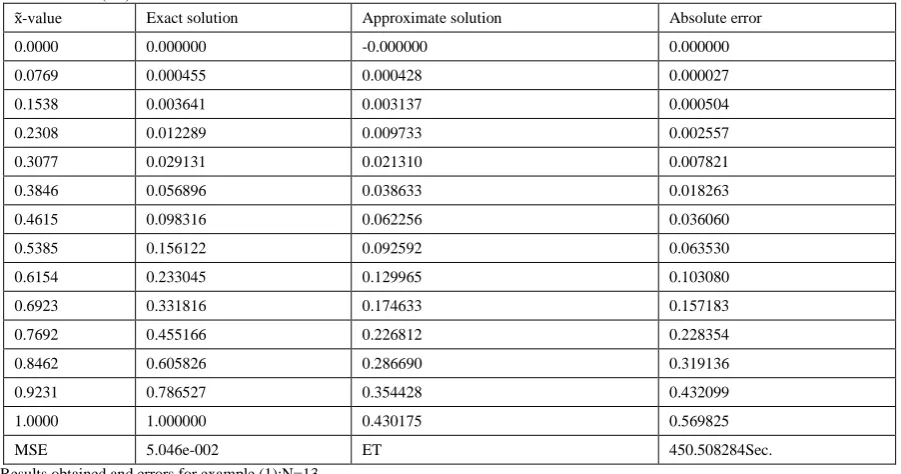
Table1: illustrate the comparison between the exact and the approximate solution depending on Mean Square Error(MSE) and Elapsed Time (ET).

x̃-value Exact solution Approximate solution Absolute error

0.0000 0.000000 -0.000000 0.000000

0.0769 0.000455 0.000428 0.000027

0.1538 0.003641 0.003137 0.000504

0.2308 0.012289 0.009733 0.002557

0.3077 0.029131 0.021310 0.007821

0.3846 0.056896 0.038633 0.018263

0.4615 0.098316 0.062256 0.036060

0.5385 0.156122 0.092592 0.063530

0.6154 0.233045 0.129965 0.103080

0.6923 0.331816 0.174633 0.157183

0.7692 0.455166 0.226812 0.228354

0.8462 0.605826 0.286690 0.319136

0.9231 0.786527 0.354428 0.432099

1.0000 1.000000 0.430175 0.569825

MSE 5.046e-002 ET 450.508284Sec.

Results obtained and errors for example (1):N=13.

Table 2: illustrate the comparison between the exact and the approximate solution depending on Mean Square Error(MSE) and Elapsed Time (ET).

x̃-value Exact solution Approximate solution Absolute error

0.0000 0.000000 -0.000000 0.000000

0.0667 0.000296 0.000282 0.000014

0.1333 0.002370 0.002090 0.000280

0.2000 0.008000 0.006549 0.001451

0.2667 0.018963 0.014463 0.004500

0.3333 0.037037 0.026415 0.010622

0.4000 0.064000 0.042839 0.021161

0.4667 0.101630 0.064065 0.037564

0.5333 0.151704 0.090354 0.061349

0.6000 0.216000 0.121914 0.094086

0.6667 0.296296 0.158919 0.137378

0.7333 0.394370 0.201515 0.192856

0.8000 0.512000 0.249830 0.262170

0.8667 0.650963 0.303978 0.346985

0.9333 0.813037 0.364062 0.448975

1.0000 1.000000 0.430175 0.569825

MSE 4.913e-002 ET 1721.679419Sec.

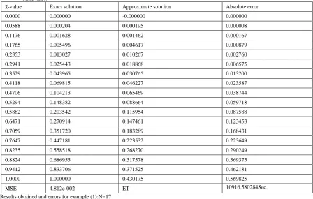
Table 3: illustrate the comparison between the exact and the approximate solution depending on Mean Square Error(MSE) and Elapsed Time (ET).

x̃-value Exact solution Approximate solution Absolute error

0.0000 0.000000 -0.000000 0.000000

0.0588 0.000204 0.000195 0.000008

0.1176 0.001628 0.001462 0.000167

0.1765 0.005496 0.004617 0.000879

0.2353 0.013027 0.010267 0.002760

0.2941 0.025443 0.018868 0.006575

0.3529 0.043965 0.030765 0.013200

0.4118 0.069815 0.046227 0.023587

0.4706 0.104213 0.065469 0.038744

0.5294 0.148382 0.088664 0.059718

0.5882 0.203542 0.115954 0.087588

0.6471 0.270914 0.147461 0.123453

0.7059 0.351720 0.183289 0.168431

0.7647 0.447181 0.223532 0.223649

0.8235 0.558518 0.268270 0.290249

0.8824 0.686953 0.317578 0.369375

0.9412 0.833706 0.371525 0.462181

1.0000 1.000000 0.430175 0.569825

MSE 4.812e-002 ET 10916.580284Sec.

Results obtained and errors for example (1):N=17.

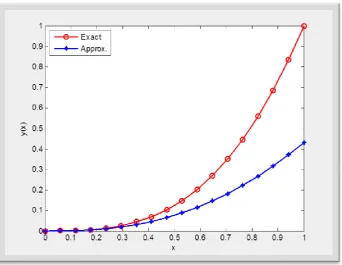
Fig. 4:A Comparison between the exact and the approximate solution using expansion method of Chebyshev polynomials of the first kind of application forN=15.

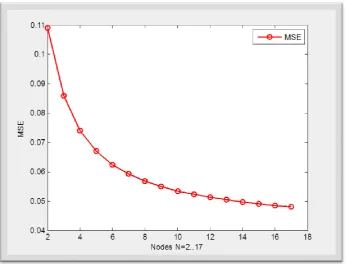
Fig. 6: A Comparison between the Shifted Chebyshev nodes and the MSE of application when N=2….14.

Conclusions:

In this paper, we have submitting expansion method using Chebyshev polynomials of the first kind of degree n as basis function for approximating the solution of one weakly singular integro-differential equation: which is the LVWSIDEs.In the application we have reduced the solution of LVWSIDEs to thesystem of linear equations by removing the singularity using an approximate point t, andwe have the following results:When the degree of expansion method of Chebyshev polynomials of the first kind is increases the error is decreases. Which is shown in Tables (1), (2) and (3).As well asthe proposed method is a delicate and an effective to solve LVWSIDEs.Finally this method can be extended and applied to the system of LVWSIDEs.

REFERENCES

. Brunner, H., 1983. “Non polynomial spline collocation for Volterra equations with weakly singular kernels”, SIAM J. Numer. Anal., 20: 1106-1119.

Brunner, H., A. Pedas and G.Vainikko, 2001. “A spline collocation method for linear integro-differential equations with weakly singular kernels”, BIT 41: 891-900.

Brunner, H., A. Pedas, G. Vainikko, 1999. The piecewise polynomial collocation method for nonlinear weakly singular Volterra equations, Math Comp., 68: 1079-1095.

Mason, J.C., D.C.Handscomb, 2003. “Chebyshev Polynomials”, Boca Raton London New York

Washington.

Mehrdad Lakestani, Behzad Nemati Saray and Mehdi Dehghan, 2011. “Numerical solution for the weakly singular Fredholm integro-differential equations using Legendre multiwavelets”, J. Comput. Appl. Math., 235: 3291-3303.

Palamora, A., 1996. Product integration for Volterra integral equations of the second kind with weakly singular kernels,Math. Comp. 65(215): 1201-1212.

Qinghua Wu, 2014. “The Approximate Solution of Fredholm Integral Equations with Oscillatory Trigonometric kernels”, Article ID 172327,7pages.