Hourly wind speed forecasting based on support vector machine and artificial neural networks

ISSN: 2252-8938, DOI: 10.11591/ijai.v8.i3.pp286-291  286

Hourly wind speed forecasting based on support vector machine

and artificial neural networks

Laboratory of High Energy Physics-Modeling and Simulations, Rabat, Morocco

Article Info ABSTRACT

Article history: Received May 17, 2019 Revised Jul 27, 2019 Accepted Aug 23, 2019

Wind speed is the main component of wind power. Therefore, wind speed forecasting is of big importance due to its uses. It permits to plan the dispatch, determine the hours of storage needed, the amount of energy stored that should be used and avoid the big fluctuations in the electrical grid caused by the nature of the renewable energy resources. In this paper, we propose four hybrid models based on Support Vector Machine (SVM) and Artificial Neural Networks (ANNs) or just Neural Networks (NN) for wind speed forecasting. Using the Ordinary Least Squares (OLS) analysis for selecting the parameters more influencing wind speed. Then, a Support Vector Machine and Artificial Neural Networks models are tuned by Genetic Algorithm (GA) and Particle Swarm Optimization (PSO). The performance of these models is evaluated using three statistical indicators: the Mean Square Error (MSE), Mean Error (ME) and Mean Absolute Error (MAE). The results show a better performance of the neural model compared to the support vector machine.

Keywords: Genetic algorithm Neural Network

Particle swarm optimization Support vector machine Wind speed forecasting

Copyright © 2019 Institute of Advanced Engineering and Science. All rights reserved. Corresponding Author:

Soukaina Barhmi,

Laboratory of High Energy Physics-Modeling and Simulations, Rabat, Morocco.

Email: soukainabarhmi90@gmailcom

1. INTRODUCTION

Wind power is nowadays one of the predominant alternative energy sources since the energy produced by wind is clean, also it helps in reducing global warming and environmental pollution because it doesn't emit dangerous emissions (e.g., those produced by fossil fuel power stations that cause several human health issues). In this sense, the accurate forecast of wind speed is important for the safety of renewable energy utilization. At the present time, Morocco is the largest producer of wind power in Africa since it benefits from great solar and wind energy potential [1] because of its key geographic location [2]. In recent years, many methods have been developed to forecast wind speed. Classical and hybrid models [3] were subject to many works. In [4] presented a hybrid model that consisted of the Ensemble Empirical Mode Decomposition (EEMD) and the Genetic Algorithm- Backpropagation (GA-BP) neural network and compared their performance to Empirical Mode Decomposition (EMD) and the Genetic Algorithm-Backpropagation (GA-BP), traditional Genetic Algorithm-Algorithm-Backpropagation (GA-BP) and Wavelet Neural Network method (WNN) and The best model found was the hybrid EEMD and GA-BP neural network method (6.82% for MAPE and 0.59 for RMSE). On the other hand, in [5] designed a new hybrid model KF-ANN based on the artificial neural network (KF-ANN) and Kalman filter (KF) and compared to Autoregressive Integrated Moving Average (ARIMA), Artificial Neural Network (ANN), hybrid ARIMA-KF models, the results showed that all these models were effective but the MAPE values indicated that the hybrid KF-ANN model was the most effective. In [6] exploited ANN and compared with persistence and ARIMA, the best model was a backpropagation network with one hidden layer and nine neurons (0.18 m/s for MAE and 0.05m2/s2 for MSE). In [7] applied the evolutionary-SVM algorithm for short-term wind speed prediction in

wind turbines of Spanish wind farm. In [8] presented a combination method PSO-BP neural network and the results indicate that the proposed method is effective for the wind speed prediction more than the basic back propagation neural network and ARIMA model.

Artificial neural networks based methods [9-10] prove to be the best for nonlinear problems due to its capacity of generalization and fitting any kind of functions which makes it suitable for any random variable based process in particular forecasting the renewable energy resources. Due to their nonlinear nature, artificial neural networks are used as part of the many forecasting hybrid model and we choose the SVM because it is shown to be efficient in addressing nonlinear input-output mapping [11]. On the other hand, the simplicity and flexibility of GA and PSO justify its use to optimize the NN connection weights and SVM parameters during the training phase. In this study, we find based on the Ordinary Least Squares (OLS) analysis four inputs influencing the wind speed, namely, direction, humidity, temperature and past wind speed. The data handled are the hourly meteorological satellite data from 2011 to 2013 (3 years) provided by the Research Institute of Solar Energy and New Energy (IRESEN). The region studied is Tangier located in the south Mediterranean ocean (located in the latitude 35.800, longitude –5.840 and altitude 8 in north Morocco). Afterwards, we apply the proposed hybrid models SVM-GA, SVM-PSO, NN-GA and NN-PSO to capture the relationship between the aforementioned inputs and the wind speed and to verify the performance of these models for the prediction of hourly wind speed in Tangier. The remainder of this article is organized as follows: Section 2 discusses in details the NN, SVM, GA and PSO. In section 3 experimental results analysis are given in detail, and the last section concludes this article.

2. METHODOLOGY

In this section, the methodologies and algorithms used for prediction are presented. The first subsection will be dedicated to technique used for analyzing the inputs. The remaind subsections will handle the Support Vector Machines, Artificial Neural Network and defining each algorithms used, namely, Genetic Algorithm and Particle Swarm Optimization.

2.1. The ordinary least squares (OLS)

The ordinary least squares (OLS) is a statistical method that fits a model using all of the independent variables. It estimates the linear regression coefficients by minimizing the vertical squared distance between the regression line and the data points [12-13]. In our models, no constant will be used because it affects the results since it has no meaningful physical interpretation.

2.2. Support vector machines

Support Vector Machines (SVMs) [14-19] are supervised learning models commonly used for classification problems. Given a set of data, the SVM will attempt to separate the two classes using a hyperplane, which is a subspace one dimension less than the ambient space. Various mathematical techniques such as dual quadratic programming and non-linear kernel transformations can be used to maximize the margin between the classes of data. A hard-margin SVM will enforce the principle that the data must be separable. However, it may not be possible to achieve perfect separation of the data in some cases. Therefore, a soft-margin SVM classifier can be used to maximize the hyperplane margin while allowing some misclassifications. In our approach, we adopt ε-Support Vector Regression (ε-SVR), the basic principle of SVM for regression is to map the data into a high dimensional feature space via nonlinear mapping, after which a linear regression is performed in this feature space. The regression formula can be expressed as:

f(x)= ∑𝑁𝑖=1𝑤𝑖Ф𝑖(x)+ b (1)

where {Ф𝑖(𝑥)}𝑖=1𝑛 are named features and b is the bias term. The coefficients {𝑤𝑖}𝑖=1𝑛 can be obtained from the data by optimizing the following quadratic programming problem:

Minimize 1 2‖𝑤‖

2_{+ 𝐶 ∑ (𝜉}

𝑖+ 𝜉𝑖∗ 𝑛

𝑖=1 )

Subject to {

𝑦𝑖− 〈𝑤, Ф(𝑥𝑖)〉 − 𝑏 ≤ 𝜀 + 𝜉𝑖

〈𝑤, Ф(𝑥𝑖)〉 − 𝑦𝑖+ 𝑏 ≤ 𝜀 + 𝜉𝑖∗

𝜉𝑖≥ 0, 𝜉𝑖∗≥ 0, 𝑖 = 1, … … . 𝑛

(2)

where 𝜉𝑖∗ is a slack variable and C is a positive constant determining the trade off between the flatness of 𝑓 and the amount up to which deviations larger than ε are tolerated. Here, by solving the optimization problem through the introduction of Lagrange multipliers and optimality constraints:

f(χ, α, α∗_{) = ∑ (α}

i−αi∗) k(xi, x) D

i=1 + b (3)

where 𝛼𝑖𝑎𝑛𝑑 𝛼𝑖∗ are called Lagrange multipliers. They are obtained by maximizing the dual function of (2) as follows:

Maximize∑𝑛𝑖=1𝑦𝑖(𝛼𝑖−𝛼𝑖∗) − 𝜀 ∑𝑛𝑖=1(𝛼𝑖+ 𝛼𝑖∗) − 1

2∑ ∑ (𝛼𝑖− 𝛼𝑖

∗_)(𝛼

𝑗−𝛼𝑗∗)𝐾(𝑥𝑖, 𝑥𝑗 𝑛

𝑗=1 𝑛

𝑖=1 )

Subject to {∑ (𝛼𝑖−𝛼𝑖

∗_{) = 0} 𝑛

𝑖=1

0 ≤ 𝛼𝑖, 𝛼𝑖∗≤ 𝐶

(4)

For k(𝑥𝑖, 𝑥𝑗), it denotes the kernel function equal to the inner product of two vectors 𝑥𝑖𝑎𝑛𝑑 𝑥𝑗 in the feature space Ф(𝑥𝑖)𝑎𝑛𝑑 Ф(𝑥𝑗), given by k( 𝑥𝑖, 𝑥𝑗) = Ф(𝑥𝑖). Ф(𝑥𝑗). Any function that satisfies Mercer’s condition [20] can be used as the kernel function and hence it depends on the problem at hand. In our approach, we opted Radial Basis Function (RBF) as the kernel function of SVR model with good analyticity and arbitrary rank derivatives existence, good performance under general smoothness assumptions. Further details concerning the ε-SVR are presented in [21] and the expression of radial basis function is.

𝑘(𝑥𝑖, 𝑥𝑗) = exp (− ‖𝑥𝑖−𝑥𝑗‖2

2𝜎2 ) (5)

2.3. Neural network

Neural network is the modeling and prediction tool [22]. The network forms by connecting the output of certain neurons to the input of other neurons through synaptic weights used to store the knowledge. Any layer that is formed between the input layer and the output layer is called hidden layer. The output of the neural network is given by the following equation:

𝑌 = 1

1+ exp (−𝑧) (𝑧 = ∑ 𝑋𝑖∗ 𝑊𝑖+𝑏𝑖 𝑁

𝑖=1 ) (6)

where Xi are the inputs, Wi the weights and bi are the biases. It should be noted that the number of neurons in

the input/output layer is related to the variables that are dealt with.

The input/target datasets were divided randomly into two subsets. The first set is to train the neural network using the learning algorithm in order to find the optimal weights that minimize the Mean Square Error (MSE). The second one is to validate the already trained model [23].

2.4. Genetic algorithm

A genetic algorithm is a stochastic general search method [24-27]. It was proposed by John Holland et al and widely applied in various forecasting and optimization fields. The genetic algorithm selects the individuals of random from the current population and these individuals use to produce the children for the next generation and repeatedly modifies a population of individual solutions. At each step, over successive generations, the population "evolves" toward an optimal solution.

2.5. Particle swarm optimization

The PSO is a new evolutionary computation method [28-32]. The system is initialized with a population of random solutions and searches for optima by updating generations. In PSO, the particles fly through the problem space by following the current optimum particles. The basic mathematical expressions of PSO are as follows:

𝑣𝑠𝑑(𝑡 + 1) = 𝑣𝑠𝑑(𝑡) + 𝑐1(𝑡)𝑟1(𝑡)(𝑝𝑠𝑑(𝑡) − 𝑥𝑠𝑑(𝑡)) + 𝑐2(𝑡)𝑟2(𝑡)(𝑝𝑔𝑑(𝑡) − 𝑥𝑠𝑑(𝑡))

𝑥𝑠𝑑(𝑡 + 1) = 𝑥𝑠𝑑(𝑡)+𝑣𝑠𝑑(𝑡 + 1) (7)

where t is iteration number; random variable of r1 and r2 obey uniform distribution of the interval (0, 1); c1 (t)

and c2 (t) are acceleration constants; xsd (t) is the position of the particle S in the t iterations; psd (t) is the

3. RESULTS AND DISCUSSION

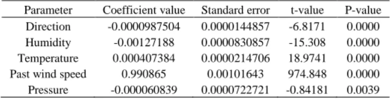
In this study, we tried to fit 5 inputs to wind speed, namely, Direction, past wind speed, Humidity, pressure and temperature, selecting the predictors is a necessary phase. In order to do that, some assumptions must be verified. The first one is to check the correlation between the dependent variable and the predictors in order to determine the degree of dependence of the predicted values to the predictors. A p-value of 0.05 or more means that it would not be rejected at the 5% level [33] and their value are given in Table 1. Consequently, you should consider removing pressure from the model of Tangier.

The second one is to remove the multicollinearity between independent variables. Finally, four explanatory independent variable most influencing wind speed are direction, humidity, temperature and past wind speed to develop the proposed hybrid models [34]. The SVM model is used to perform wind speed forecasting. The parameters, cost (C), gamma (g), epsilon (e) has a significant impact on the forecasting performance, their values are listed in Tables 2 and 3. The Genetic Algorithm (GA) and Particle Swarm Optimization (PSO) are used to optimize the above three parameters by minimizing the MSE value. To evaluate the proposed hybrid approach and to determine quantitatively the best model, the coefficient of determination (R2_{) and three statistical indices are utilized to measure the forecasting accuracy. These indices}

are the Mean Error (ME), Mean Square Error (MSE) and Mean Absolute Error (MAE) between the predicted and the actual values of wind speed, then the errors are defined as:

Table 1. Statistical analysis obtained from the OLS at Tangier station

Parameter Coefficient value Standard error t-value P-value

Direction -0.0000987504 0.0000144857 -6.8171 0.0000

Humidity -0.00127188 0.0000830857 -15.308 0.0000

Temperature 0.000407384 0.0000214706 18.9741 0.0000

Past wind speed 0.990865 0.00101643 974.848 0.0000

Pressure -0.000060839 0.0000722721 -0.84181 0.0039

Table 2. Optimal parameters of SVM-GA

City Values of parameters

Tangier Cost(C) Gamma(g) Epsilon(e)

15.2749 3.144599 0.0006444887

Table 3. Optimal parameters of SVM-PSO

City Values of parameters

Tangier Cost(C) Gamma(g) Epsilon(e)

10.8001 0.167599 0.0003052174

ME =1

N∑ (Ti−Yi N

i=1 ) (8)

MSE =1

N∑ (Ti− Yi) 2 N

i=1 (9)

MAE =1

N∑ |Ti− Yi| N

i=1 (10)

R2_{= 1 −}∑Ni=1(Ti−Yi)2 ∑N (T_i−T)2

i=1

(11) where Ti are the targets, T is the mean of all target values, Yi are the neural network outputs and N is the

number of samples.

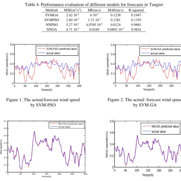
Table 4 shows the errors of the four hybrid models. The coefficient of determination (R-squared), also called goodness of fit, shows a very good quality of prediction for the NN-GA and NN-PSO models since the values are very close to 1. Additionally, the MSE, ME and MAE show a relatively low error in the models which can be explained by the fact that the models describe most of the data, but the NN-GA is the best suited for the prediction with MSE= 4.71 10-4_m2_/s2 _{with 3 neurons in the hidden layer. On the other}

hand, the R-squared of SVM-GA and SVM-PSO models is very close to 0. However, the MSE, ME and MAE show a relatively low error in the models which can be explained by the fact that the models describe most of the data but not with a high accuracy. Furthermore, Figure 1 and Figure 2 show a large gap between actual and predicted SVM-GA and SVM-PSO values, but in Figure 3 and Figure 4 the two curves are almost confused for NN-GA and NN-PSO. According to these results, we conclude that the NN-GA is able to predict the wind speed with a higher accuracy than the other models.

Table 4. Performance evaluation of different models for forecasts in Tangier

Methods MSE(m2_/s2_{) ME(m/s) MAE(m/s) R-squared}

SVMGA 2.42 10-2 _{6 10}-3 _{0.1238 0.1947}

SVMPSO 2.60 10-2 _{1.31 10}-2 _{0.1281 0.1355}

NNPSO 5.27 10-4 _{4.0765 10}-5 _{0.0124 0.9881}

NNGA 4.71 10-4 _{0.0169 9.0892 10}-4 _0.9834

Figure 1. The actual/forecast wind speed by SVM-PSO

Figure 2. The actual/ forecast wind speed by SVM-GA

Figure 3. The actual/forecast wind speed by NN-PSO Figure 4. The actual/forecast wind speed by NN-GA

4. CONCLUSION

The objective of this study was the prediction of wind speed using four hybrid models. In the first, we find based on the OLS analysis four inputs influencing the wind speed, namely, direction, humidity, temperature and past wind speed. Afterwards, we apply the proposed hybrid models NN-GA, SVM-GA, SVM-PSO and NN-PSO to capture the relationship between the aforementioned inputs and the wind speed. The performance of these models is evaluated using R-squared and three statistical indicators: the Mean Square Error (MSE), Mean Error (ME) and Mean Absolute Error (MAE). The conclusion made is that the SVM-GA and SVM-PSO are not suitable for estimating the behavior of wind speed in the region of Tangier using the selected inputs. On the other hand, the nonlinear method of neural networks tuned by genetic algorithm using the same inputs gives excellent results which indicate its high accuracy in the prediction of wind speed.

REFERENCES

[1] Kingdom of Morocco (2009). Moroccan Regions 2010. http://www.hcp.ma/downloads/Maroc-en-chiffres_t13053.html. Last checked on Dec 29, 2017.

[2] Kingdom of Morocco (2011). Moroccan Investment Development Agency.http://invest.gov.ma/. Last checked on Dec 29, 2017.

[3] J. S. Jung, RP. Broadwater, “Current status and future advances for wind speed and power forecasting,” Renew Sustain Energy Rev, vol. 31, pp. 762-777, 2014.

[4] S. Wang, N. Zhang, L. Wu, and Y. Wang, “Wind speed forecasting based on the hybrid ensemble empirical mode decomposition and GA-BP neural network method,” Renewable Energy, vol. 94, pp. 629–636, 2016.

0 50 100 150 200 250 300

0 0.2 0.4 0.6 0.8 Temps(h) W in d s p e e d (m /s )

SVM-PSO predicted value actual value

0 50 100 150 200 250 300

0 0.2 0.4 0.6 0.8 Temps(h) W in d s p e e d (m /s )

SVM-GA predicted value actual value

0 50 100 150 200 250 300

0 0.1 0.2 0.3 0.4 0.5 0.6 0.7 Temps(h) W in d sp ee d( m /s )

NN-PSO predicted value actual value

0 50 100 150 200 250 300

0 0.2 0.4 0.6 0.8 Temps(h) W in d s p e e d (m /s )

NN-GA predicted value actual value

[5] O. B. Shukur, and M. H. Lee, “Daily wind speed forecasting through hybrid KF-ANN model based on ARIMA,”

Renewable Energy, vol. 76, pp. 637-647, 2015.

[6] J. C. Palomares-Salas, A. Aguera-Perez, J. J. G. de la Rosa, and A. Moreno-Munoz, “A novel neural network method for wind speed forecasting using exogenous measurements from agriculture stations,” Measurement., vol. 55, pp. 295-304, September 2014.

[7] Salcedo-Sanz Sancho, Ortiz-Garcı´a Emilio G, Pérez-Bellido Ángel M, Portilla-Figueras Antonio, Prieto Luis. Short term wind speed prediction based on evolutionary support vector regression algorithms. Expert Syst Appl 2011; 38(4):4052-7.

[8] Ren Chao, An Ning, Wang Jianzhou, Li Lian, Hu Bin, Shang Duo. Optimal parameters selection for BP neural network based on particle swarm optimization: a case study of wind speed forecasting. Knowl – Based Syst 2014; 56:226-39.

[9] H.N. Wang, Y.M. Cui, R. Li, L.Y. Zhang, H. Han, “Solar flare forecasting model supported with artificial neural network techniques,” Advances in space research, vol. 42, pp. 1464-1468,3 November 2008.

[10]A. Koca, H. F. Oztop, Y. Varol, G. O. Koca, “Estimation of solar radiation using artificial neural networks with different input parameters for Mediterranean region of Anatolia in Turkey,” Expert systems with applications, vol. 38, pp. 8756-8762, 2011.

[11]E. Ghysels, and H. Qian, “Estimating MIDAS Regressions via OLS with a Polynomial Parameter Profiling,” Econometrics and Statistics.Cortes, vol. 9, pp. 1-16, 2018.

[12]D. G. Kleinbaum, L. L. Kupper, and K. E. Muller, “Applied Regression Analysis and Other Multi-variable Methods,” PWS Publishing Co., Boston, MA, USA, 1988.

[13]C, Vapnik V N, “Support vector networks. Machine Learning,” vol. 20, pp. 273-297, 1995.

[14]H.M. Pei, Y. Y Chen, Y.K. Wu,” Laplacian total margin support vector machine based on within-class scatter,”

Knowledge-Based Systems, vol. 119, pp. 152-165, 2017.

[15] Ch. Sudheer, R. Maheswaran,B. K. Panigrahi, “A hybrid SVM-PSO model for forecasting monthly streamflow,”

Neural Computing and Applications, vol. 24(6), pp. 1381-1389, 2014.

[16] SC. Huang, B. Chen,” Automatic moving object extraction through a real-world variable-bandwidth network for traffic monitoring system,” IEEE Transactions on Industrial Electronics, vol. 61(4), pp. 2099-2112, 2014.

[17] JX. Wu, “Efficient HIK SVM learning for Image Classification,” IEEE Transactions on Image Processing, vol. 21(10), pp. 4442-4453, 2012.

[18] F. Zhu, N. Ye, W. Yu, “Boundary detection and sample reduction for one-class support vector machine,”

Neurocomputing, vol. 123, pp. 174-184, 2014.

[19] J.X. Du, D.S.Huang, X.F. Wang, X. Gu, “Shape recognition based on neural networks trained by differential evolutionalgorithm,” Neurocomputing, vol. 70(4-6), pp. 896-903, 2007.

[20]D. Basak, S. Pal, “Patranabis DC Support vector regression,” Neural Inf Process Lett Rev, vol. 11, pp. 203-224, 2007.

[21]AJ. Smola, B. Sch¨olkopf, “A tutorial on support vector regression,” Stat Comput, vol. 14, pp. 199–222, 2004. [22]SA. Kalogirou, “Artificial neural networks in renewable energy systems applications: a review” Renew Sust Energy

Rev, vol. 5(4), pp. 373–401, 2001.

[23]B. Curry, and D. E. Rumelhart, “An MSnet: A Neural Network which Classifies Mass Spectra,” Tetrahedron Computer Methodology, vol.3, pp. 213-237, 1990.

[24]D. Liu, D. Niu, M. Xing, Q. Nie,” Day-ahead price forecast with genetic-algorithm-optimized support vector machines based on garch error calibration,” Automation of Electric Power Systems, pp. 31-40, 2007.

[25]S. Marsili-Libelli, P. Alba. Adaptative mutation in genetic algorithms. Soft Comput 2000; 4:76-80.

[26]JE. Baker. Reducing bias and inefficiency in the selection algorithm, genetic algorithms and their applications. Proc of the Second Int Conf on Gen Alg 1987:14-21.

[27]JR. Fernández, JA. López-Campos, A. Segade, JA. Vilán. A genetic algorithm for the characterization of hyperelastic materials. Appl Math Comput 2018; 329:239-50.

[28]R. Jursa, K. Rohrig,”Short-term wind power forecasting using evolutionary algorithms for the automated specification of artificial intelligence models,” International Journal of Forecasting, vol.24, pp. 694-709, 2008. [29]J. Kennedy, R. Eberhart, Particle swarm optimization, Neural Networks, 1995.In: Proceedings. IEEE International

Conference on, November/December 1995, 4, Perth, WA, vol. 1944, pp. 1942–1948.

[30]R. Eberhart, J. Kennedy, A new optimizer using particle swarm theory, MicroMachine and Human Science, 1995. MHS ’95, in: Proceedings of the SixthInternational Symposium on, 4–6 October 1995, Nagoya, Japan, pp. 39-43. [31]R.C. Eberhart,Y.H. Shi, Particle swarm optimization: Developments,applications and resources, in: Proceedings of

the 2001 Congress onEvolutionary Computation, Vols 1 and 2, 27–30 May 2001, Seoul, SouthKorea, pp. 81-86. [32]R.C. Eberhart, Y.H. ve Shi, Special issue on Particle Swarm Optimization, in: IEEE Transactions on Evolutionary

Computation, June 2004. pp. 201-203

[33]C. Dougherty, Introduction to Econometrics, Oxford University Press, USA, 2007.

[34]S. Barhmi, O. El fatni, I. Belhaj,” Forecasting of wind speed using Multiple Linear Regression and Artificiel Neural Networks”, Energy Syst (2019). https://doi.org/10.1007/s12667-019-00338-y.