CORRECTING REFERENCE BIAS IN HIGH-THROUGHPUT SEQUENCING ANALYSIS
Shunping Huang
A dissertation submitted to the faculty of the University of North Carolina at Chapel Hill in partial fulfillment of the requirements for the degree of Doctor of Philosophy in the Department of
Computer Science.
Chapel Hill 2015
Approved by:
Wei Wang
Leonard McMillan
Vladimir Jojic
Fernando Pardo-Manuel de Villena
ABSTRACT
SHUNPING HUANG: Correcting Reference Bias in High-throughput Sequencing Analysis (Under the direction of Wei Wang)
Mapping reads to a reference sequence is a common step when analyzing high throughput sequencing data. The choice of reference is critical because its effect on quantitative sequence analysis is non-negligible. Recent studies suggest aligning to a single standard reference sequence, as is common practice, can lead to an underlying bias depending the genetic distances of the target sequences from the reference. To avoid this bias researchers have resorted to using modified reference sequences. Even with this improvement, various limitations and problems remain unsolved, which include reduced mapping ratios, shifts in read mappings, and the selection of which variants to include to remove biases.
ACKNOWLEDGEMENTS
I would like to express my deepest gratitude to my advisor Dr. Wei Wang for her support and guidance during my Ph.D. journey. She has encouraged my study and provided me lots of constructive suggestions on research and career development. I am also very thankful to Dr. Leonard McMillan for inspiring me with new thoughts and ideas in every discussion we had. I thank Dr. Fernando Pardo Manuel de Villena for the collaboration oppotunity and his insightful advices on my research projects. I am also grateful to Dr. Vladimir Jojic and Dr. Wei Sun for their invaluable feedbacks on my dissertation.
Many of my research projects were joint efforts with other collaborators, so my appreciation extends to them, the members in COMPGEN group and CEGS group. I thank Dr. Xiang Zhang for his helps during my first few years of research. I also thank Dr. Yi Liu, Zhaojun Zhang, Andrew Parker Morgan, Weibo Wang, Wei Cheng, James Matt Holt, Chia-Yu Kao, Zhaoxi Zhang, Jack Wang, and many other UNC graduate students for supporting my work in these years.
I was funded by SAS Institute in the last year of my Ph.D. research. I am so thankful for their internship opportunity. I would like to thank my former manager Taiyeong Lee for the trust and support. I also thank my colleages in SAS for such a great working environment.
TABLE OF CONTENTS
LIST OF TABLES . . . ix
LIST OF FIGURES . . . x
LIST OF ABBREVIATIONS . . . xii
1 Introduction . . . 1
1.1 Basic Biology . . . 1
1.2 High-throughput Sequencing . . . 4
1.3 Alignment . . . 5
1.3.1 Reference Sequence . . . 5
1.3.2 Genomic Variation. . . 6
1.4 Related Work on Reference Bias . . . 7
1.5 Contributions . . . 9
1.5.1 Thesis Statement . . . 9
1.5.2 Organization . . . 10
2 MOD Format . . . 11
2.1 Design of the MOD format . . . 11
2.2 Properties of the MOD format . . . 12
2.2.1 Invertibility . . . 12
2.2.2 Concatenability. . . 13
2.2.3 Composability . . . 14
2.2.4 Other properties . . . 14
2.3 Use of the MOD format . . . 14
2.3.2 Position Mapping . . . 15
2.3.3 Application in Mouse Genome . . . 15
3 Novel Alignment Pipelines . . . 23
3.1 Single Reference Pipeline . . . 23
3.2 Alignment Pipeline for Inbreds . . . 24
3.2.1 Pseudogenome Construction . . . 25
3.2.2 Pseudogenome Alignment and Annotation . . . 26
3.2.3 Result on RNA-seq read alignment of inbred mice . . . 28
3.2.4 Result on DNA-seq read alignment of inbred mice . . . 31
3.3 Multi-Alignment Pipeline for F1s . . . 33
3.3.1 Pseudogenome Alignment and Annotation . . . 33
3.3.2 Merging - Comparing Alignments . . . 33
3.3.3 Merging - Filter Pipeline . . . 35
3.3.4 Result on RNA-seq read alignment of F1 mice . . . 38
3.3.4.1 Comparison of Mapping Ratio . . . 38
3.3.4.2 Comparison of Parental Origin Labeling . . . 39
3.3.4.3 Performance of Merging . . . 43
4 Handling Remaining Bias . . . 45
4.1 Preliminary . . . 45
4.2 Probabilistic Model for Common Trend and Outliers . . . 47
4.2.1 Objective Function . . . 48
4.2.2 Polishing . . . 49
4.2.3 Tuningλ. . . 50
4.2.4 Ranking Outliers . . . 50
4.3 Results . . . 52
4.3.1 Simulation Experiments . . . 53
4.3.1.2 Outlier Detection . . . 54
4.3.2 Experiment on DNAseq Data . . . 57
5 Summary and Future Directions . . . 63
5.1 Summary . . . 63
5.2 Future Directions . . . 63
LIST OF TABLES
2.1 Statistics of MOD files for CAST, PWK and WSB . . . 16
2.2 Percentage of exons, transcripts, and genes with different lengths . . . 17
3.1 Number of reads for 12 samples from 3 inbred strains . . . 28
3.2 Percentage of RNA-seq reads mapped to pseudogenomes and the reference . . . 29
3.3 Percentage of RNA-seq reads with observed variants . . . 30
3.4 Comparison of mapping positions and CIGAR strings . . . 30
3.5 Comparison between Tophat 1.4.0 and Tophat 2.0.6 . . . 31
3.6 Percentage of DNA-seq reads mapped to the pseudogenome and the reference . . . 32
3.7 Breakdown percentage of reads that mapped to both genomes . . . 32
3.8 Number of reads for 10 samples from F1s . . . 38
3.9 Comparison of Parental origin of reads from CAST×PWK samples. . . 41
3.10 Comparison of Parental origin of reads from PWK×CAST samples. . . 41
4.1 Notation Table . . . 48
4.2 Table forRSSnormal(φmin= 1.5,φmax= 3.0) . . . 55
LIST OF FIGURES
1.1 Mouse Karyotype . . . 2
1.2 DNA Transcription and Translation . . . 3
1.3 RNA Splicing . . . 4
1.4 RNA-seq Procedure . . . 5
1.5 Transition and Transversion . . . 6
1.6 Examples of Indels . . . 7
1.7 Examples of Structural Variations . . . 7
2.1 A MOD file Example . . . 12
2.2 Three Main Properties of the MOD Format . . . 18
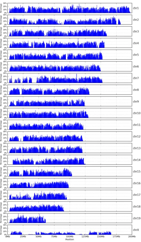
2.3 High-variant intervals of CAST pseudogenome . . . 19
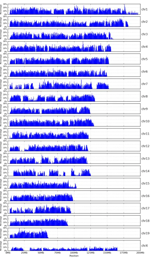
2.4 High-variant intervals of PWK pseudogenome . . . 20
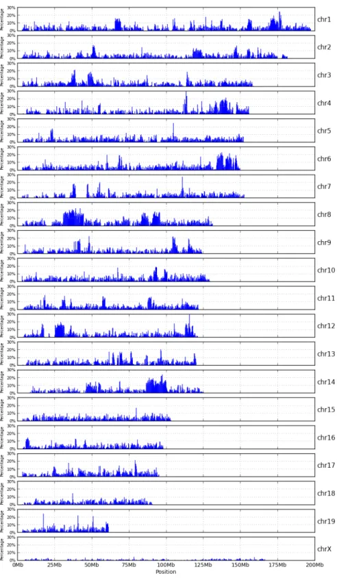
2.5 High-variant intervals of WSB pseudogenome . . . 21
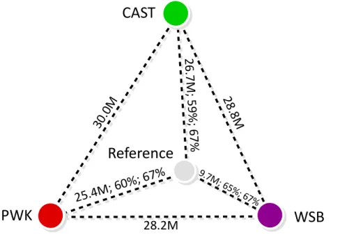
2.6 Estimated genetic distances between the reference and three strains . . . 22
3.1 Single Reference Pipeline . . . 24
3.2 Inbred Pipeline . . . 25
3.3 Multi-Alignment Pipeline for a diallel cross . . . 34
3.4 Filter Steps in Multi-alignment pipeline . . . 36
3.5 Mapping ratio and unique mapping ratio of reads . . . 39
3.6 Percentage of parental origin labels in different pipelines . . . 40
3.7 Average filter distribution of mapped reads . . . 42
3.8 Average parent-of-origin distribution of autosome mapped reads . . . 43
4.1 An example of three synthetic data sets under different assumptions: (a)the same read coverage across samples, (b)different read coverages for different samples, and (c)different read coverages for different samples with outliers. . . 47
4.2 Examples of outliers in local read depth . . . 51
4.4 Box plots of∆µ(φmin = 3.0,φmax= 6.0) . . . 55
4.5 ROC plots (φmin = 1.5,φmax= 3.0) . . . 59
4.6 ROC plots (φmin = 3.0,φmax= 6.0) . . . 59
4.7 An illuatration of the FVBx(WSBxPWK) strain . . . 60
4.8 Estimated common trends for FVB/PWK samples in chr2:73.8Mbp-87.3Mbp . . . 60
4.9 Venn diagram of Top 20/40 outliers . . . 61
LIST OF ABBREVIATIONS
DNA Deoxyribonucleic acid RNA Ribonucleic acid mRNA Messenger RNA rRNA Ribosomal RNA tRNA Transfer RNA
cDNA Complementary DNA DNA-seq DNA Sequencing RNA-seq RNA Sequencing
SNP Single Nucleotide Polymorphism CNV Copy Number Variation
RIL Recombinant Inbred Line MLE Maximum Likelihood Estimate MAP Maximum a posteriori
STD Standard Deviation
CHAPTER 1: INTRODUCTION
It is well known that the biological information of all organisms and many viruses is stored in deoxyri-bonucleic acid (DNA) composed of nucletides. This information plays an essential role in the suvival, development, and reproduction of an organism. Since 1970s, researchers have been using all kinds of sequencing approaches to determine the order of nucleotides and unwind the secret of DNA. While in the early days sequencing was prohibitively time-consuming, labor intensive, and expensive, its cost has been dramatically brought down by the recent advance of high-throughput sequencing technology, making it universally accessible to average labs. Nowadays, sequencers generate huge volumnes of raw reads, which then should be further analyzed.
There are two common strategies for processing raw reads: alignment and assembly. Given that the procedure of assembly is usually memory- and time-consuming, many researchers are inclined to use alignment approaches. One of the prerequisites of alignment is the reference sequence, to which reads are mapped. While the standard reference sequence of an organism is commonly used in alignment, it is not always guaranteed that the target organisms match exactly the standard reference. Ignoring such difference may result in bias during read alignment, namely reference bias.
In this chapter, I first introduce some basic biology, which should be sufficient for average readers to understand the rest of my dissertation. Then I present the alignment procedure, reference sequence, and genomic variants. I also survey some related work on reference bias.
1.1 Basic Biology
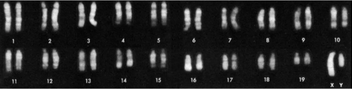
DNA wrapped with proteins is organized into thread-like structures calledchromosomes. There are two types of chromosomes based on whether they control somatic characters or sex characters. The former type is calledautosomes, and the latter typesex chromosomes. The entire set of chromosomes, which contains all genetic information of an organism, is called thegenomeof this organism. The number of chromosomes in a genome is different for differentplodies(i.e. the number of sets of chromosomes in a cell) and species. For example, among diploid organisms, where chromosomes are in pairs, humans have 23 pairs of chromosomes, including 22 pairs of autosomes and 1 pair of sex chromosomes; mice have 20 pairs of chromosomes, where 19 of them are autosomes and the remaining pair are sex chromosomes (Figure 1.1).
Figure 1.1: Mouse Karyotype (Committe on Standardized Genetic Nomeclature for Mice, 1972). The mouse genome has 19 pairs of autosomes and one pair of sex chromosomes.
DNA controls the organism’s cells and body through a multi-step process called protein synthesis. However, not all of the genomic sequence is functional in this process. The region that is functional and corresponding to a unit of inheritance is called agene, and the region that does not encode protein sequence is called noncoding DNA. Protein synthesis consists of two major steps,transcriptionand translation (Figure 1.2), and involves three types ofribonucleic acid (RNA)–messenger RNA (mRNA),ribosomal RNA (rRNA), andtransfer RNA (tRNA).
Figure 1.2: DNA Transcription and Translation are the two major steps in protein synthesis. The genetic code of DNA is first transcribed to mRNA and then translated into amino acids. (http://www.ignyc.com/ our-work/portfolio/transcription-translation/)
the discarded ones are calledintrons. For a given gene, there can be different ways of splicing, also called alternative splicing, which will result in different mRNA sequences being produced.
Figure 1.3: RNA Splicing. The exons are remained in the mature mRNA, while the introns are removed.
(http://en.wikipedia.org/wiki/RNA_splicing)
1.2 High-throughput Sequencing
Sequencing technologies always have a great impact on the research of sequence analysis. In the early decades, sequencing was a time-consuming and money-consuming process, since it was hardly automated and could only determine a few sequence each time. Recent development of high-throughput sequencing technologies has allowed sequencing processes to be run in parallel. This has dramatically lowered down the cost of DNA sequencing, making it accessible to labs of different sizes in the research community. So far, high-throughput sequencing technologies have been widely used in the studies of whole genome sequencing (DNA-seq), transcriptome profiling (RNA-seq), DNA-protein interactions (ChIP-seq), etc.
Figure 1.4: RNA-seq Procedure. The mRNA molecules from a sample is extracted, purified, and reversely transcribed to cDNAs. Then cDNAs are sequenced by the sequencer machine to produce reads.
1.3 Alignment
Read alignment(or simplyalignment) is the process of figuring out the localtion of each read in areference sequence, which is a very long sequence served as a template. After reads are obtained from the sequencer, alignment is the preferred way of read processing, since it requires less time and memory than assembly.
Analigneris a piece of code/tool that performs the alignment procedure. For each read in a given set, an aligner will try to find its location in the reference sequence. If such a location can be found, it is called amappingof this read. A read mapping is not guaranteed to match the exact sequence of the read. Some aligners can allow certain amounts of mismatches or gaps. In the end, there are three different outcomes while aligning a read: (a) only one location is found, which is also called aunique mapping; (b) more than one location is found, i.e.multiple mappings; (c) no location is found, namelyno mapping.
1.3.1 Reference Sequence
A common prerequisite of nearly all sequence analysis pipelines is to align read fragments to a high-quality reference genome sequence, regardless of the underlying organism’s ploidy. This reference sequence/genome is usually called thestandard reference sequence/genomeof this organism.
et al., 2012), functional elements (The ENCODE Project Consortium et al., 2011), and genetic variants (The 1000 Genomes Project Consortium, 2010; Keane et al., 2011) are given in coordinates relative to a reference genome.
1.3.2 Genomic Variation
Although the reference sequence for one species is high-quality, it cannot represent the sequence of every samples from this species. The difference between the standard reference and the target organism is called genomic variation.
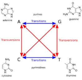
Genomic variation can be separted into different types based on the size and the effect on the genome. Single Nucleotide Polymorphisms (SNPs) A SNP is a point mutation which causes a substitution of a single nucleotide with another. There are two categories of point mutation: transitions and transversions (Figure 1.5). Transitions occur about ten times more often than transversions.
Figure 1.5: Transition and Transversion. Transition represents the conversion between A and G (purine to purine) or C and T (pyrimidine to pyrimidine), while transversion represents the other combinations.
(http://en.wikipedia.org/wiki/Transition_(genetics))
Insertions or Deletions (Indels) An indel represents an insertion or deletion of bases in the sequence (Figure 1.6).
Figure 1.6: Indel examples (http://blog.hackbrightacademy.com/2013/07/ indel-finder-how-the-python-version-of-this-program-works/)
A translocationoccurs when a large chromosome region is exchanged with another large chromosome region. Aninversionhappens when one chromosome breaks in two different locations, and the middle part of sequence is reversed and re-attached to the chromosome. The examples of different types of structure variation are shown in Figure 1.7.
Figure 1.7: Examples of Structural Variations.(http://hodnett-ap.wikispaces.com/Chapter+23+ The+Evolution+of+Populations/)
1.4 Related Work on Reference Bias
et al., 2010; Peng et al., 2012). Whereas ascertaining copy-number and calling genomic variants are common DNA-seq quantitative analysis examples.
While the standard reference genome is widely used in read alignment, the quality of the alignment decreases as measured by the numbers of unmapped and misaligned fragments, as the genetic distance between the reference and target genomes increases. Also, aligning reads to a reference genome can introduce local alignment biases, (i.e., regions that better match the reference sequence tend toward higher coverage than regions with variations (Degner et al., 2009; McDaniell et al., 2010)) which largely confounds downstream quantitative analyses.
Many researchers have addressed this issue by incorporating variants, to various extents, into apseudo -reference genome sequence. Incorporating only SNPs is commonplace and straightforward (Satya et al., 2012), since it does not change the coordinates of the constructed genome sequence. Alternatively, Degneret al. (Degner et al., 2009) masked every known polymorphic location in the reference genome by introducing a third allele, thus increasing the genetic distance between the target and the reference in an unbiased fashion. However, this approach reduces the total number of reads aligned because the added masked alleles always introduce mismatches, which all aligners attempt to minimize. In fact, unmapped reads result when the best mapping considered has excessive mismatches. In RNA-seq experiments, this reduction in mapped reads leads to underestimation of expression level of genes with variations(Turro et al., 2011).
There have also been some attempts to utilize other variants besides SNPs. Rivas-Astrozaet al. (Rivas-Astroza et al., 2011) developed a software (perEditor) to build a personal genome with different variant types, but they only focussed on genome construction without resolving the coordinate inconsistency after read alignment.
The problem is getting even worse if the target organism is non-inbred. When parental haplotypes differ in their similarity to the reference sequence a significant alignment bias can result. Gregget al. (Gregg et al., 2010) aligned F1 hybrids from reciprocal crosses between the isogenic mouse strains CAST/EiJ and C57BL/6J to the NCBI37/mm9 mouse genome and transcriptome to study parent-of-origin effects. However, this approach favors reads with reference alleles, and it is worth noting that the mouse reference genome is largely based on C57BL/6J.
C57BL/6J-based reference genome and an approximate DBA/2J genome where known DBA/2J variants, primarily SNPs, were substituted into the reference. Turroet al. (Turro et al., 2011) proposed a hybrid pipeline that first aligned reads to a reference genome in order to call SNPs, and then re-aligned the same reads to a customized transcriptome with the discovered SNPs incorporated. Since single-base substitutions do not change genome coordinates, it is straightforward to embed SNPs. However, this method cannot be easily generalized to other frame-shifting variants such as small indels, inversions and CNVs to which a sequence aligner is more sensitive. Rozowskyet al. (Rozowsky et al., 2011) proposed AlleleSeq for constructing a modified diploid genome by inserting SNPs and indels into the reference genome and using this diploid genome as the reference during alignment to avoid errors caused by reference bias. While AlleleSeq is similar to one of my proposed pipelines, it is limited to diploid organisms. Moreover, as shown below, it analyzes differential expression at variant positions, which will become more difficult as the density of variants increases.
After reads are mapped, the relative read counts in specific regions of the sequence are often used to quantify abundance within a genomic region. In DNA sequencing (DNA-seq), local read counts are used to estimate copy-number gain or loss (Yoon et al., 2009; Magi et al., 2012). In RNA sequencing (RNA-seq), local read counts are used to quantify gene expression levels and to identify the isoforms expressed (Richard et al., 2010; Turro et al., 2011). In diploid organisms, researchers have been interested in assessing the differential expression levels between parental haplotypes, (i.e., parent-of-origin or allele effects). In a typical analysis of differential expression, the read coverage at each known variant position are partitioned by allele and then used to estimate the imbalance (Gregg et al., 2010; Keane et al., 2011; Rozowsky et al., 2011). Statistical corrections to the read counts are required when the density of local variations allows multiple variants to fall in the same read, or read-pair. Thus, in regions with dense genomic variations, the quantitative use of read counts is complicated both by the inability to align, and by the difficulty of establishing the independence of each variant observation.
1.5 Contributions
1.5.1 Thesis Statement
reference bias than the traditional pipeline where reads are mapped against the standard reference sequence. They can be applied to a wide range of organisms, including inbreds, F1s, and outbreds. Performance is measured by the ratio of mapped or uniquely mapped reads as well as the distribution of reads among different founders.
1.5.2 Organization
The remainder of my dissertation is organized as follows:
• Chapter 2presents a general variation format between genomes, which plays an important role in the pipelines I proposed.
• Chapter 3presents the new alignment pipelines for different types of organisms to correct reference bias.
• Chapter 4presents a probabilistic model to handle remaining bias by common trend estimation and outlier detection.
CHAPTER 2: MOD FORMAT
In this chapter, I propose a general framework for mapping coordinates back and forth between genomes. It employs a new format, namely MOD format, to represent known variants between genomes. This format greatly facilitates genome construction and position mapping, and is the key component in the pipelines for correcting reference bias in Chapter 3.
2.1 Design of the MOD format
The MOD format is composed of instructions that transform one genome sequence into another. It is essentially an edit transcript relating two strings (Gusfield, 1997), and it provides a basis for quantifying the similarity of two sequences. A MOD file is not necessarily unique, nor is it claimed to be minimal. The genome before transformation is called thesourceand the one after is called thedestination. Each MOD file is directional, i.e. always from the source to the destination.
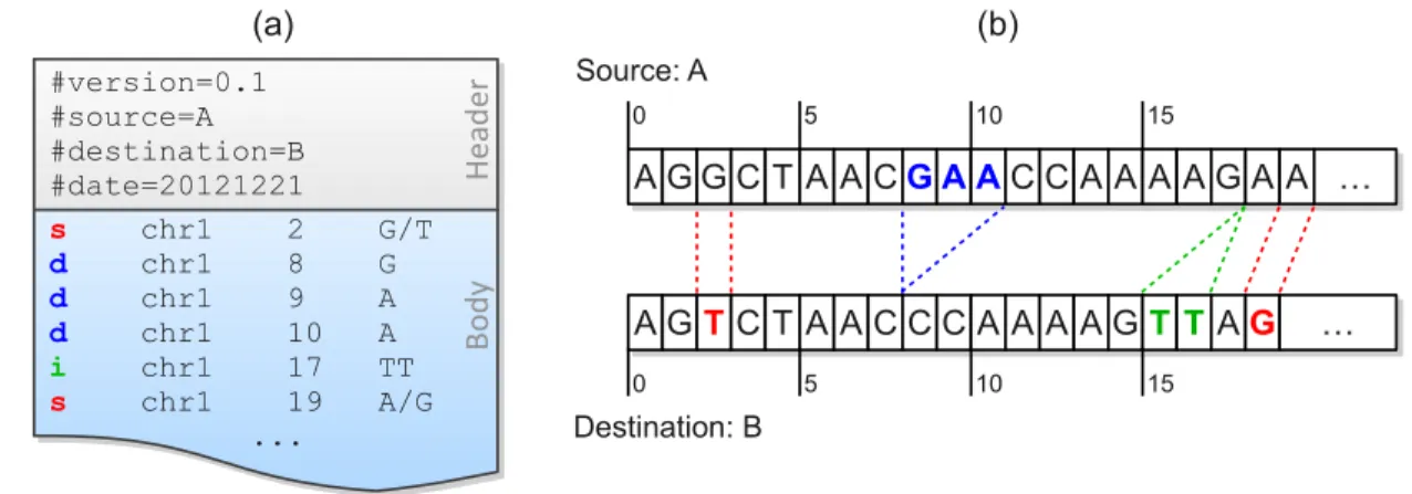
A MOD file consists of two parts (Figure 2.1a): a header and a body. The header includes the metadata of the transformation, such as, the version of the MOD format, the source, the destination, and so forth. The body holds the instructions, each of which has its affected position and arguments. Positions are all stored in the source coordinate system, and the bases before and after modification are included in the arguments.
There are three basic types of instructions defined in the MOD format: s-,d-, andi-instructions. They describe single-base substitutions, single-base deletions, and insertions, respectively. All instructions are atomic, in that they reference no more than one position from the source. It is obvious that both s-instructions and d-instructions are atomic. For i-instructions, I merely add new sequence after an anchor position in the source without altering any base; thus they are also atomic.
choice of keeping all instructions atomic facilitates later MOD-file manipulations, whose advantages are considered to outweigh this slight redundancy. Moreover, the additional space overhead is recovered when MOD files are compressed.
Complex structure variants, such as tandem duplications, inversions, and translocations, can be described by the current set of instructions. For example, a tandem duplication is represented by repeating an i-instruction at the same location, while inversions (or translocations) are implemented by a series of d-instructions at the source sequence position and a corresponding i-instruction of the inverted (or transferred) sequence at its new position. It is recommended to annotate such coupled sets of instructions using comments following the instructions.
New MOD files can also be derived from other MOD files by various properties of the format. This will be discussed in Section 2.2 .
0 5 10 15
A
AGGGGCCTTAAAACCGGAAAACCCCAAAAAAAAGGAAAA ……
A
AGGTTCCTTAAAACCCCCCAAAAAAAAGGTTTTAAGG 0
…
…
5 10 15
Source: A Destination: B (a) (b) #version=0.1 #source=A #destination=B #date=20121221 #version=0.1 #source=A #destination=B
#date=20121221 Hea
de
r
s chr1 2 G/T d chr1 8 G d chr1 9 A d chr1 10 A i chr1 17 TT s chr1 19 A/G ...
s chr1 2 G/T d chr1 8 G d chr1 9 A d chr1 10 A i chr1 17 TT s chr1 19 A/G ...
Bo
dy
Figure 2.1: A MOD file example (a) and the corresponding sequences of the source and the destination (b). There are two SNPs between these sequences, and they are represented as two s-instructions at source positions 2 and 19. A three-base deletion (from source positions 8 to 10) is observed, and it is broken up into three d-instructions. The insertion after position 17 is directly added to the MOD file without any conversion due to its atomicity.
2.2 Properties of the MOD format
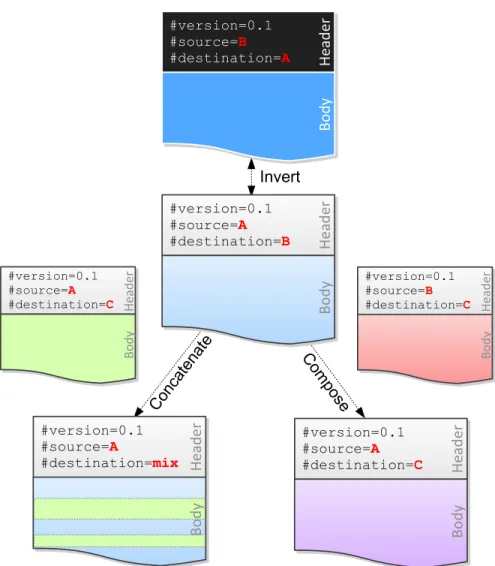
2.2.1 Invertibility
For example, each s-instruction specifies a position and a nucleotide from the source and its replacement nucleotide in the destination, so it can be inverted by merely swapping the two nucleotides. The d-instructions contain bases that they remove from the source, so inverting them will result in inserting these deleted bases back to the destination, i.e. i-instructions. Moreover, since d-instructions are restricted to be one-based but i-instructions are not, adjacent i-instructions can be combined into one as an optimization. Similarly, i-instructions are broken up into multiple d-instructions While they are inverted.
The position of each instruction must also be modified when inverting a MOD file. Positions in the source coordinate system are changed into destination coordinates in the output as described in Section 2.3.2 .
2.2.2 Concatenability
The MOD files with the same source genome can be concatenated. In other words, one can combine a prefix sequence generated from one MOD file with a suffix sequence from another MOD file without messing up the coordinates or missing any variants on the segment boundaries, as long as the two MOD files have the same source (Figure 2.2). Concatenation is used to construct new genomes for hybrid organisms (e.g., F2s and backcrosses) to account for recombinations.
Concatenability results from the use of atomic instructions in a single source coordinate system. Given a genomic region, every instruction in a MOD file will be either inside or outside the region; there is no case where an instruction crosses a region boundary. Therefore, unlike variant calls that require special care in the boundary cases, MOD files can be safely cropped.
2.2.3 Composability
Given two MOD files containing instructions to transform genomeAto genomeB and genomeBto genome C, respectively, one can construct a MOD file transforming genome Ato genomeC (Figure 2.2). This property is called composability.
LetP(A7→B)andQ(B 7→C)represent the two MOD files to be composed, andR(A7→C)be the resulting MOD file. The procedure of composition is briefly described as follows. First, we invertPto obtainP0, which contains instructions mapping from genomeB to genomeA. Second, we compute the intersection ofP0andQ, i.e.,P0∩Q. These shared instructions indicate thatAandCare identical at the corresponding positions, because same changes should be made to changeB toAandBtoC. Third, we remove the intersection fromP0andQobtainingP¯0andQ¯ separately. These two MOD files are the actual
difference betweenAandC. Finally, we map the instruction positions inQ¯ from genomeB coordinates to genomeAcoordinates (described in Section 2.3.2), and combine the result with the inversion ofP¯0. This gives the expected MOD fileR.
2.2.4 Other properties
In addition to these three properties, the MOD format has other virtues. For example, it can be easily converted from the VCF format (Danecek et al., 2011), which is commonly used to store variant calls. Also, the MOD files can be compressed by bgzip (Li et al., 2009) and indexed by tabix (Li, 2011), so that the file sizes are reduced and they can be efficiently queried.
It is also convenient to edit a MOD file to incorporate new variants or to mask obsolete ones. Since all positions are in the same coordinate system for each MOD file, there is no need to worry about adjusting positions when adding or removing variants.
2.3 Use of the MOD format
2.3.1 Genome Construction
One can easily construct MOD files for entire catalogs of common inbred strains using readily available variant calls. The property of concatenability makes it convenient to create the pseudogenomes for arbitrary crosses between inbred strains and recombinant inbred lines (RILs)(Silver et al., 1995). The genomes of RILs are a mosaic of two or more founder genomes. Once the haplotype structure of a RIL is inferred (Liu et al., 2010; Fu et al., 2012), one can concatenate the regions of instructions from founder MOD files to form a new MOD file for the RIL, which can then be utilized for alignments.
When using MOD files it is often assumed that there is a common source genome, or reference, but this restriction is unnecessary. The MOD format can be used to map between any two genomes or genome versions, allowing the source sequence to be transformed to any destination sequence.
2.3.2 Position Mapping
The MOD format also provides the capability to map coordinates or intervals from the source to the destination, and vice versa. This is done by scanning a MOD file and accumulating the number of shifted bases affected by d-instructions and i-instructions. For every pair of corresponding regions in the two genomes, I record a pair of offsets. Given a position in the source, I first look up in the source offsets to find out in which region it falls, and then compute its destination position.
The invertibility of the MOD files guarantees that one can map positions back and forth between the source and the destination. The composability also extends the mapping ability. For example, given two MOD files, from the reference to two non-reference strains, one can invert one and compose them to get a third. With the help of this MOD file, one can map positions between the two non-reference strains.
Position mapping can be applied to genome annotations, which is usually presented in the reference coordinate system, to get a new target-specific annotation. Position mapping can also be applied to genome alignment results, so one can remap the alignments from one genome to another.
2.3.3 Application in Mouse Genome
Here I used the mouse as the model organism, but the MOD format and the tools I proposed are also applicable to other organisms.
Strain s-instructions d-instructions i-instructions CAST 17,674,364 4,834,899 4,206,776 PWK 17,202,935 4,715,249 3,457,436 WSB 6,045,875 2,026,461 1,579,714
Table 2.1: Statistics of MOD files for CAST/EiJ, PWK/PhJ and WSB/EiJ. The counts are in units of base-pairs. For s-instructions and d-instructions, they are just the numbers of instructions, respectively. For i-instructions, the counts are derived from adding up the number of bases in each inserted sequence.
The SNP and indel variants for these strains were downloaded from the Wellcome Trust Sanger Institute (Keane et al., 2011), while the mouse reference genome data is from NCBI MGSCv37.
To generate MOD files for the three target strains, I first extracted SNPs and indels from the VCF files (downloaded fromftp://ftp-mouse.sanger.ac.uk/REL-1105/). Only high-confidence SNPs and indels for the 19 autosomes and X were incorporated into the MOD files. Variants on Y and mitochondria (M) were extracted from other sources (http://cgd.jax.org/datasets/popgen/ diversityarray/yang2009.shtml). The MOD files used in this paper can be found at http: //www.csbio.unc.edu/CCstatus/index.py?run=Pseudo. I summarized the statistics for each MOD file in Table 2.1.
The total number of bases involved in all instructions of a MOD file can be used as an estimation of genomic distance between a strain and the reference. Figure 2.6 shows such distance for the three strains studied. The CAST strain is the most distant genetically from the reference and the WSB strain is the genetically closest to the reference.
Strain Exons Transcripts Genes
CAST 5.98% 78.04% 62.37%
PWK 5.87% 76.68% 61.42%
WSB 3.01% 65.76% 52.75%
Table 2.2: Percentage of exons, transcripts, and genes that have different lengths in the pseudogenomes. I also constructed strain-specific gene annotations for the CAST, PWK and WSB pseudogenomes, and investigated how many exons, transcripts, and genes were changed after variants were incorporated in the reference.
The gene annotation of mm9 was from Ensembl (Flicek et al., 2012). There are, in total, 688,311 exons, 97,251 transcripts, and 37,620 genes in the latest release (release 67).
To accomplish this, I developed a tool,modmap, for mapping positions and intervals from source to the destination. It takes a MOD file and an annotation file as input. It first builds a position mapping between genomes internally and then changes the annotation file’s position columns from source coordinates to destination coordinates. In the current setting, the source is the reference genome, and the destination is the pseudogenome.
After the strain-specific annotation was obtained, I compared it with the original annotation in terms of the start positions and the ranges of exons, transcripts, and genes.
Not surprisingly, because of the integrated indels and structure variants, the start positions of almost all exons, transcripts and genes (over 99%) are shifted in the pseudogenome annotation. In addition, about 6% of exons, 78% of transcripts and 62% of genes have different lengths in the CAST pseudogenome (Table 2.2). There is a strong correlation between the number of changes in a strain and the genetic distance of the strain from the reference (Figure 2.6).
Invert
Con cate
nate Com
po se #version=0.1 #source=B #destination=A #version=0.1 #source=B
#destination=A Hea
de r Bo dy #version=0.1 #source=A #destination=B #version=0.1 #source=A
#destination=B Hea
de r Bo dy #version=0.1 #source=A #destination=C #version=0.1 #source=A
#destination=C Hea
de r Bo dy #version=0.1 #source=A #destination=C #version=0.1 #source=A
#destination=C Hea
de r Bo dy #version=0.1 #source=B #destination=C #version=0.1 #source=B
#destination=C Hea
de r Bo dy #version=0.1 #source=A #destination=mix #version=0.1 #source=A
#destination=mix Hea
de
r
Bo
dy
CAST
WSB
26
.7
M
; 5
9%
; 6
7%
25.4M
; 60%
; 67%
9.7M; 65%; 67%
PWK
Reference
30
.0
M
28
.8M
28.2M
CHAPTER 3: NOVEL ALIGNMENT PIPELINES
In this chapter, I describe my pipelines for correcting reference bias on inbred and multi-parental sequencing data. For comparison purposes, I also consider a traditional analysis pipeline that employs a single reference genome and attempts to achieve similar annotations. In all fairness, this single-reference pipeline is only an approximation to the front-ends of other published methods. I have deliberately attempted to separate the annotation phase of sequence analysis from subsequent analyses. Assessments of the differential expression levels due to parent, allele, or slice variants are considered downstream uses of the annotations. I contrast my approaches with the representative reference-based pipeline and highlight their major differences.
3.1 Single Reference Pipeline
In traditional reference-based alignment pipelines, short-reads from high throughput sequencers are first mapped to a standard reference genome or sequence(Figure 3.1) and genetic variation is considered afterward. There are significant advantages in using the standard reference. In addition to supplying a common coordinate system for comparison between target genomes, reference coordinates anchor nearly all of the genome’s functional annotations, such as gene/exon locations, transcription factor binding sites, and notations of common variants. When all samples are aligned to this reference, genomic comparisons are significantly simplified. However, the mappability to the reference genome is reduced if a sample has a large number of variations from the reference. This results in either a reduction in the number of reads mapped and/or an increase in mapping errors. If the number of errors exceeds the aligner’s tolerance, the read will be simply dropped from the output and its information will be lost. In short, a sample that is genetically distant from the reference will typically align fewer reads and with reduced confidence than a sample that is closer to the reference.
Raw reads
Raw reads
Aligner
Aligner
Read alignments
Read alignments
Reference Reference
Figure 3.1: The single reference pipeline is the traditional way of read alignment. The standard reference sequence is directly used by the aligners for read alignment.
with the maternal strain but only one with the paternal one, the single-reference pipeline assumes that the mapping is from the maternal side. If such counts are the same, suggesting an equal chance of coming from either one, then the strain origin of this mapping cannot be determined.
3.2 Alignment Pipeline for Inbreds
Aligning read fragments to a reference genome or transcriptome sequence is subject to reference bias. Starting from inbred organisms, which is both simple and commonly used in experiments, I propose the following new alignment pipeline to correct reference bias.
Executing the instructions of a MOD file for an inbred organism, incorporates variants into the reference genome sequence to obtain a pseudogenome. Reads can then be mapped to the pseudogenome using an alignment tool such as Tophat (Trapnell et al., 2009) or Bowtie (Langmead et al., 2009; Langmead and Salzberg, 2012). The aligned read file (typically a BAM file) can then be remapped back to the reference genome’s coordinates for analysis using the same MOD file. I developed a tool for this purpose calledLapels, which remaps the positions of the read fragment alignments, modifies their associated CIGAR string, and annotates the variants seen in each fragment (Figure 3.2) .
Raw reads Raw reads
Aligner Aligner
MOD file MOD file Pseudogenome
Pseudogenome
Lapels Lapels
Read alignments (remapped to reference)
Read alignments (remapped to reference)
Read alignments Read alignments
Reference
Reference
MOD Interpreter
MOD Interpreter
Figure 3.2: Inbred Alignment Pipeline. Instead of using the standard reference for alignment, the inbred pipeline takes the pseudogenome, which is constructed from the MOD file and the standard reference, as the reference and performs read alignment. After read alignments,Lapelswill convert the positions of each reads from pseudogenome coordinates back to standard coordinates.
strains. It is convenient to have a common coordinate system so that comparisons between strains will become feasible.
3.2.1 Pseudogenome Construction
Given a MOD file, it is easy to transform one source sequence to another destination sequence. In my experiments MOD files were mainly derived from known genetic variants (SNPs, insertions, and deletions) of several wild-derived mice. Therefore, pseudogenomes for these mice were generated based on the mouse standard reference sequence and MOD files.
1: functionBUILDSEQ(chrom, chromLen, srcSeq) 2: instructionSet←LoadInstructions(chrom) 3: srcP os←0
4: dstSeq←00
5: for allinst∈instructionSetdo 6: insP os←inst.position 7: ifsrcP os < insP osthen
8: dstSeq+ = srcSeq[srcP os:insP os] 9: srcP os←insP os
10: end if
11: Execute Instructionson PositioninsP os 12: end for
13: ifsrcP os < chromLenthen
14: dstSeq+ = srcSeq[srcP os:chromLen] 15: end if
16: returndstSeq 17: end function
reference genome, so the end result of alignment is a BAM file (Li et al., 2009) using the coordinate system of the pseudogenome.
3.2.2 Pseudogenome Alignment and Annotation
Separate alignments create problems when comparing samples. If I tried to compare a CAST/EiJ inbred to a PWK/PhJ inbred using only the pseudogenome alignments, there would be two different genomic coordinate systems in play.
To alleviate this issue, I use the same set of known allelic differences incorporated into the pseudogenome to translate all of the mapped reads back to the reference coordinate system. This involves going through each mapped read and adjusting the mapping position, cigar string, and edit distance to match the reference genome instead of the pseudogenome. This step is done by a program calledLapelsin my pipeline.
1: functionREMAPREADS(chrom) 2: readSet←LoadReads(chrom)
3: instructionSet←LoadInstructions(chrom) 4: regionM ap←BuildMapping(instructionSet) 5: for allr ∈readSetdo
6: Look upr.positioninregionM apand getdelta 7: r.position+ = delta
8: Save and adjustr.cigar, tagN M (edit distance) 9: end for
10: returnreadSet 11: end function
12: functionBUILDMAPPING(instructionSet) 13: srcP os←0
14: delta←0
15: regionM ap← {}
16: for allinst∈instructionSetdo
17: Insert(srcP os→delta)intoregionM ap 18: ifinst.typeis s-instructionthen
19: srcP os+ =inst.length
20: continue
21: else ifinst.typeis i-instructionthen 22: delta+ = inst.length
23: else ifinst.typeis d-instructionthen 24: srcP os+ =s.length
25: delta−= inst.length 26: end if
27: end for
28: Insert(srcP os→delta)intoregionM ap 29: returnregionM ap
3.2.3 Result on RNA-seq read alignment of inbred mice
The sequenced mouse samples were derived from the aforementioned wild-derived mouse strains. Over 1.2G reads were sequenced on the Illumina HiSeq 2000 platform of mRNA from the brain tissue extracted from 12 samples (4 samples per strain) using paired-end reads with 100 bp (2x100). The number of reads per sample is shown in Table 3.1 .
Table 3.1: Number of reads for 12 samples from 3 inbred strains.
Strain Sample 1 Sample 2 Sample 3 Sample 4 Total CAST 88,520,554 78,903,440 78,976,480 135,080,364 381,480,838 PWK 140,642,004 96,388,598 96,735,248 132,859,376 466,625,226 WSB 130,888,744 123,814,138 66,178,922 92,044,920 412,926,724
I used TopHat (v.1.4.0), with default parameter settings, to map reads to pseudogenomes derived from MOD files and the NCBI MGSCv37Mus musculusreference genome.
After aligning, the read fragments from the resulting BAM files were remapped back to the reference genome and tagged with the number of observed variants (i.e., the number of variants incorporated in the pseudogenome and observed in the read). Based on the number of alignments in the resulting BAM file, we categorized each read into one of the three classes: unmapping (0), unique mapping (1), and multiple mapping (>1).
I also aligned the same reads to the standard reference genome and compared them to the reads mapped to the pseudogenome. The percentage of reads by category and the average percentages of biological replicates are shown in Table 3.2 .
Observe that more reads map uniquely to the pseudogenome than to the reference (shaded cells). The percentage increase is 7.46% for CAST, 6.76% for PWK, and 2.38% for WSB.
On one hand, the percentage of reads that uniquely map to the reference increases as we move from CAST (59.35%) to PWK (60.43%) to WSB (65.02%). This again accurately reflects the genetic distance of each strain from the reference (Figure 2.6) . The more different that a strain is from the reference, the fewer of its reads are mapped to reference genome, thus illustrating a reference bias.
Table 3.2: Average percentage of RNA-seq reads from CAST, PWK, and WSB samples mapped to the pseudogenome and the reference. (Tophat 1.4.0, Bowtie 0.12.8)
Alignment Reference
Unique Multiple Unmapped Total
CAST Pseudogenome
Unique 58.91% 0.10% 7.80% 66.81% Multiple 0.11% 2.31% 0.01% 2.43% Unmapped 0.33% 0.01% 30.42% 30.76% Total 59.35% 2.42% 38.23% 100.00%
PWK Pseudogenome
Unique 60.01% 0.09% 7.09% 67.19% Multiple 0.14% 2.37% 0.01% 2.52% Unmapped 0.28% 0.01% 30.00% 30.29% Total 60.43% 2.47% 37.10% 100.00%
WSB Pseudogenome
Unique 64.83% 0.04% 2.53% 67.40% Multiple 0.06% 2.47% <0.01% 2.54% Unmapped 0.13% <0.01% 29.93% 30.06% Total 65.02% 2.52% 32.46% 100.00%
of reads remain unmapped, I believe this residual represents current limitations of the aligner in combination with the remaining inaccuracies in the pseudogenome sequence.
Notice that the largest percentage increase is due to reads that were mapped uniquely to the pseudognome but unmapped to the reference (cells with pink shading). This suggests that my pipeline has rescued many reads that are discarded in the traditional method, especially when the strain is distant from the reference.
In order to understand how the embedded variants affect the alignment result, I investigated what percentage of reads have observed variants in the each categories and summarized the result in Table 3.3. Notice that categories involving unmapped reads in pseudogenomes are not included in the table, because such reads have no alignment and, thus, no observed variants of the strains.
Table 3.3: Average percentage of RNA-seq reads with observed variants from CAST, PWK, and WSB samples in each category.
Alignment Reference
Unique Multiple Unmapped Total CAST Pseudogenome Unique 21.50% 64.59% 88.74% 29.58% Multiple 74.99% 2.74% 78.80% 6.10% PWK Pseudogenome Unique 21.68% 61.38% 88.08% 28.85% Multiple 76.46% 4.01% 77.48% 8.22% WSB Pseudogenome Unique 7.79% 56.51% 84.25% 10.71% Multiple 75.96% 2.42% 78.37% 4.40%
Table 3.4: Comparison of mapping positions and CIGAR strings for reads uniquely mapped to both genomes. Strain Unequal Start Equal Start but Unequal CIGAR Equal Start and CIGAR
CAST 0.32% (82.43%) 0.41% (97.70%) 99.26% (20.98%) PWK 0.32% (79.78%) 0.39% (97.41%) 99.29% (21.20%) WSB 0.12% (79.03%) 0.20% (97.62%) 99.68% (7.53%)
Of those reads that mapped uniquely in both the reference and pseudogenomes, only a small fraction of them contain the strain-specific variants. This is to be expected since there are plenty of conserved regions in the genome. If reads originate from one of these regions, it is possible that they will be mapped uniquely to both genomes without any observed variant. Moreover, both alignments of this kind of reads should have the same mapping position, because I remapped the pseudogenome-aligned reads back to the reference coordinate system. In order to verify my hypothesis, I looked further into this category of reads by comparing the two alignments in terms of their positions and CIGAR strings. As shown in Table 3.4 , over 99% of reads in this category have the same mapping position and CIGAR string in both alignments, which justifies my previous assumption. I also observed that a large portion of remaining reads contain variants, the percentage of which is shown in parenthesis. Lastly, I found that for such reads fewer mismatches were seen in the pseudognome alignments than in the reference alignments, suggesting a better alignment result is achieved by using the pseudogenome.
Table 3.5: A comparison between Tophat 1.4.0 (with Bowtie 0.12.8) and Tophat 2.0.6 (with Bowtie 2.0.5)
Alignment Aligner Tophat 1.4.0 Tophat 2.0.6
Strain CAST PWK WSB CAST PWK WSB
Pseudogenome
mapping 69.24% 69.71% 69.94% 72.49% 72.44% 72.82% unique mapping 66.81% 67.19% 67.40% 69.41% 6927% 69.96% multiple mapping 2.43% 2.52% 2.54% 3.08% 3.17% 2.85% no mapping 30.76% 30.29% 30.06% 27.51% 27.56% 27.18% Standard
Reference
mapping 61.77% 62.89% 67.54% 67.20% 68.03% 69.32% unique mapping 59.35% 60.43% 65.02% 64.17% 64.96% 66.24% multiple mapping 2.42% 2.47% 2.52% 3.03% 3.07% 3.08% no mapping 38.23% 37.11% 32.46% 32.80% 31.97% 30.68%
Although I was able to map more reads using the newer version, the overall result is still consistent: pseudogenome alignments recover more reads and these alignments exhibit a reduced reference bias (Table 3.5). This suggests that different aligners can all benefit from my approach. My claims are that any aligner can significantly benefit from a reference sequence that better reflects the given sample, and that improving an aligner’s tolerance to errors and gaps is no panacea.
3.2.4 Result on DNA-seq read alignment of inbred mice
My inbred alignment pipeline can also be used to align DNA-seq short reads. In this experiment, the DNA-seq data set was provided by the Wellcome Trust Sanger Institute (ftp://ftp-mouse.sanger.ac.uk/ current_bams/), in which mouse strains were sequenced with Illumina HiSeq platform with over 40-fold coverage. Reads are 100bp paired-end.
I extracted the raw reads from the BAM file of CAST/EiJ and obtained 646,514,920 reads in total. Then I realigned them to both the standard reference genome and the CAST pseudogenome using Bowtie (v.2.0.5). Default parameter settings were used, and the aligner only reported the best alignment for each read. The comparison of read alignments to the pseudogenome and the reference genome is shown in Table 3.6 .
Table 3.6: Percentage of DNA-seq reads from CAST samples mapped to the pseudogenome and the reference.
Alignment Reference
Mapped Unmapped Total CAST Pseudogenome
Mapped 95.74% 0.74% 96.48%
Unmapped 0.04% 3.47% 3.51%
Total 95.78% 4.21% 100.00%
Table 3.7: Breakdown percentage of reads that mapped in both genomes. N M1 andN M2 are the edit
distances from read alignments to the CAST pseudogenome and the reference, respectively. N M1< N M2 N M1=N M2= 0 N M1=N M2>0 N M1> N M2 Total
Same Pos. 36.19% 30.70% 24.01% 0.10% 91.00%
Same Chrom. Diff. Pos. 1.78% 0.28% 0.59% 0.17% 2.81%
Diff. Chrom. 0.41% 0.56% 0.62% 0.35% 1.94%
mappability than the short fragments that are separated by exon junctions as in RNA-seq reads. Second, the tolerance of mismatches and gaps is different between Bowtie and Tophat. With default settings, as used in the experiments, Bowtie allows more mismatches than Tophat.
I further investigated the 95% of reads by grouping them based on alignment positions and edit dis-tances. For each read, I compared the alignments to the pseudogenome with those to the reference genome. Alignments are considered to occupy the same position only if their starting positions and CIGAR strings are identical. The edit distance is represented by the NM tag of each alignment. I show the results in Table 3.7 . On one hand, 91% of the reads aligned to exactly the same position. While over 54% of the reads have no mismatches or an equal edit distance in the two alignments, about 36% of the reads aligned to the reference genome have a larger edit distance than the same read’s alignment to the pseudogenome. It is worth mentioning that this percentage may vary for different aligner parameter settings and may also be influenced by noise. On the other hand, around 4.7% of the reads have different alignment locations. Since I have incorporated known variants into the pseudogenome, it is expected that the alignment positions in the pseudogenome are more accurate than those in the standard reference.
3.3 Multi-Alignment Pipeline for F1s
In this part, I move my experiments from inbred to another type of organisms, F1s, and present my pipeline for annotating multi-parental sequencing data. For the purpose of discussion, it is assumed that the data set being analyzed is RNA-seq from a two-founder diallel cross. The diallel produces samples from crossing two isogenic parental genomes. My pipeline is not limited to analyzing diallels, nor is it limited to RNA-seq analysis. The new pipeline consists of multiple alignments that incorporate all known genetic variants into a genomic model followed by annotation and merging.
One of the flaws with the single reference pipeline, applied to an entirely homozygous inbred sample, is the fact that the alignment process does not take into account known sequence differences between the given inbred and the reference. Instead, this is typically handled later during analysis or as a post-alignment annotation (as described in Section 3.1). One of the major differences in my new pipeline is to take advantage of known allelic differences as early in the pipeline as possible.
3.3.1 Pseudogenome Alignment and Annotation
Alignments are more difficult to assess for multi-parental crosses and diploid organisms in general because there are multiple sets of allelic differences to influence the alignment. In a diallel sample, there are two sets of allelic differences to take into account. I addressed this problem by constructing pseudogenomes for all contributing founder genomes, performing separate alignments of the full data set to each pseudogenome, and remapping them back to a reference genome while annotating differences as shown in Figure 3.3.
3.3.2 Merging - Comparing Alignments
Next, I considered all annotated alignments as input and merged them into a single output by choosing the best mapping for each read. This was performed bySuspendersin my pipeline (Holt et al., 2013). Suspenders sorts the BAM files by read name and systematically compares each alternative mapping. For each read, it extracts all mappings from each Lapels-annotated BAM file before comparing the results. As explained earlier, information from the original pseudogenome alignment is preserved by the annotation step.
Aligner Aligner MOD file MOD file Raw reads Raw reads Pseudogenome Pseudogenome Lapels Lapels Read alignments with reference coordinates Read alignments with reference coordinates Read alignments with pseudogenome coordinates Read alignments with pseudogenome coordinates Reference Reference Aligner Aligner MOD file MOD file Pseudogenome Pseudogenome Lapels Lapels Read alignments with reference coordinates Read alignments with reference coordinates Read alignments with pseudogenome coordinates Read alignments with pseudogenome coordinates Reference Reference Suspenders Suspenders Read alignments (merged) Read alignments (merged)
Maternal-Side Alignment Paternal-Side Alignment
Merging
MOD Interpreter
MOD
Interpreter InterpreterMOD
MOD Interpreter
Figure 3.3: Multi-Alignment Pipeline for a diallel cross. Here it is assumed that the organisms being considered are diploid. The first step is to create two pseudogenomes using the list of known allelic differences, align the same reads to both pseudogenomes, and convert the mappings back to the reference coordinate system. Next I merge the two alignments and keep only the best mappings to either pseudogenome in the final merged file.
For paired-end reads of a fragment, parental origins are “linked”. The main idea is that if one read from a fragment can be assigned to a parent unambiguously, it is inferred that its mate also came from that same parent, even if the mate contains no informative variants. To illustrate the significance of linking, in the example single-reference pipeline (Section 3.1), each read is treated independently during the annotation step even if it is mapped as a paired-end read, thus requiring the presence of an informative allele in the read to assign its origin. This approximates the common process of examining alignments only at informative variant positions, while retaining the ability to detect if two variants fall on the same read. In my new pipeline, if two read mappings are properly paired, then they are treated as a single unit throughout the entire merging process. This means that 1) the mappings of two properly paired reads will be marked with the same parental origin, 2) the quality score will be calculated once based on the mismatches and indels from the paired mapping, and 3) the merge always prefers a paired-end mapping to one or two single-end mappings from the pair.
3.3.3 Merging - Filter Pipeline
Entering into the filtering section of the pipeline, one has a set of possible mappings for a given fragment where each mapping is marked with an origin flag. By sending the set through a series of filters, one removes mappings from the set until only one possible mapping remains for each fragment. Prior to filtering, Suspenders checks to see if any of the possible mappings are mated paired ends. If so, it immediately removes all unpaired mappings from consideration since a paired mapping is preferred over an unpaired one. If there are no paired-end mappings, the mappings are grouped depending upon whether they are the first or second read from the fragment, and a mapping set from each read is independently sent through the Suspenders filters. Note that the two unpaired ends of the same fragment may be filtered in different ways because they are handled separately.
1a:100
1b:100
2a:100
3b:100
4a:100
4b:90
5a:100
5b:100
Reference Coodinate System
Alignments in Maternal Pseudogenome
Alignments in Paternal Pseudogenome
5c/d:100 4a:100
4b:90
5a:100
5b:100
5c:100
5d:100
Unique Filter
5a:100
5b:100
Quality Filter
5c/d:100
Random Filter
Maternal Cannot Tell
Paternal
Quality Score
1a/b:100 2a:100 3b:100 4a:100 5b:100
Merged Output Alignments
Figure 3.4: Sample filter path for mapping sets of five reads in a diallel cross labeled such that “4b:90” is mapping “b” of read 4 with a score of 90. Prior to filtering, 1a and 1b are combined into 1a/b because they have the same position and score in both mappings. Additionally, 5c and 5d are also combined. The mapping sets of reads 1, 2, and 3 are all output by the Unique filter since there is a single positional mapping for each. The mapping sets of reads 4 and 5 have multiple mappings, so they are diverted to the Quality filter by the Unique filter. The Quality filter outputs 4a since only one mapping of read 4 has the best score (100 compared to 90). The mapping set of read 5 has three mappings with identical scores and is therefore diverted to the Random filter which chooses one mapping arbitrarily. Since there are three in the set, each one has a 33.3% chance of being chosen, with 5b being the arbitrary choice in this example.
is a function of the number of mismatches, insertions, and deletions. Only the mapping(s) with the best score are output. For example, TopHat uses the Bowtie scoring scheme (Langmead, 2013) when reporting possible mappings(Langmead and Salzberg, 2012; Langmead et al., 2009; Trapnell et al., 2009). Assume that a read aligns to multiple pseudogenomes that straddles an informative variant caused by a SNP. The mappings to pseudogenomes with the matching variant will have fewer mismatches than that to genomes with the alternate allele. Since sequencing errors are attributes of the read, they contribute mismatches equally to all pseudogenome mappings. In places with no informative alleles, an aligner will report mappings to all genomes with identical number of mismatches. Additionally, if there are multiple variants under a read’s mapping, the read may be mapped to multiple positions in the genome, but usually only the best mappings are reported. The Quality filter attempts to simulate this behavior by keeping only the best mappings and their corresponding references. Prior to the filters, identical mappings (with same coordinates and scores) were combined into a single unit. However, the mappings were not combined if their scores were different. The Unique filter treats them as two different mappings from distinct origins and passes them to the Quality filter.
Read fragments with multiple mappings (possibly to the same position) are passed to the Quality filter. For each read fragment, I regenerated the original scores of the pseudogenome mappings from the stored cigar strings and edit distances saved during the annotation phase when remapping back to the reference. If only one mapping has the best score, then that mapping is output by the Quality filter. In Figure 3.4, the mapping set of read 4 has two different mappings (one from maternal and one from paternal). The maternal mapping has a higher quality score, so it is output by the Quality filter.
Strain CAST×PWK PWK×CAST Sample1 115,936,064 119,926,340 Sample2 87,988,306 90,706,788 Sample3 142,479,432 170,423,066 Sample4 137,698,560 92,829,168 Sample5 137,953,398 93,801,072 Total 622,055,760 567,686,434
Table 3.8: Total number of reads for 10 samples from two F1 hybrid crosses.
3.3.4 Result on RNA-seq read alignment of F1 mice
I evaluated my pipeline using a full diallel cross of CAST/EiJ and PWK/PhJ. I use the notation of CAST×
PWK to represent the cross whose maternal and paternal parents are CAST/EiJ and PWK/PhJ, respectively. Likewise, the reciprocal cross is denoted by PWK×CAST.
The mRNA were first extracted from brain tissues of 10 female samples (5 for each cross). Then Illumina HiSeq 2000 platform was used to sequence the transcribed cDNA and obtained around 1.2G paired-end reads with 100bp (2x100). The number of reads per sample is shown in Table 3.8.
I followed the similar steps shown in Section 2.3.3 to generate MOD files for both CAST and PWK. Then I ran several tools with their default parameter settings in both pipelines. RNA-seq reads were aligned against the genomes by Tophat (v2.0.5). In the multi-alignment pipeline, I used Lapels (v1.0.4) to map each read coordinate back to the reference, and Suspenders (v0.2) to merge and tag mappings. Only one mapping per read was reported in the final output.
3.3.4.1 Comparison of Mapping Ratio
I examined the fraction of mapped reads from alignments to pseudogenomes, and compared it to the fraction of the same reads when mapped to the standard reference genome. Note that this is an imperfect comparison, since I considered only whether a read maps without considering the accuracy or quality of the mapping. The mapping ratios are shown in Figure 3.5.
0.5
0.6
0.7
0.8
0.9
1.0
Either
Pseudogenome
CAST
Pseudogenome
PWK
Pseudogenome
Reference
0.748
0.720
0.716
0.689
0.716
0.685
0.680
0.653
Mapping Ratio
Unique Mapping Ratio
FG
0.5
0.6
0.7
0.8
0.9
1.0
Average Ratio of All Reads
Either
Pseudogenome
PWK
Pseudogenome
CAST
Pseudogenome
Reference
0.745
0.718
0.715
0.688
0.713
0.683
0.679
0.653
GF
Figure 3.5: Mapping ratio and unique mapping ratio of reads to the reference genome, two pseudogenomes, and either pseudogenome. Using a single pseudogenome provides a gain of approximately 3% over the reference genome and using both almost doubles the gain to 6%.
If one consider whether reads mapped to either or both pseudogenomes, the combined recovery rate gain almost doubles to around 6%. To take advantage of this gain, I used a merge process to combine the two sets of alignments in the following section.
3.3.4.2 Comparison of Parental Origin Labeling
After reads are mapped, my new pipeline and single-reference pipeline next attempt to label the pseudogenome origin of every read where possible. This is a crucial step for downstream analyses which leverage the labels to determine differential gene expression between the parental strains.
0.0
0.2
0.4
0.6
0.8
1.0
Single
Reference
Pipeline
Multi-Alignment
Pipeline
0.083
0.131
0.084
0.132
0.458
0.405
CAST(F)
PWK(G)
Can't tell
FG
0.0
0.2
0.4
0.6
0.8
1.0
Average Fraction of All Reads(Autosomes only)
Single
Reference
Pipeline
Multi-Alignment
Pipeline
0.084
0.132
0.084
0.132
0.455
0.400
GF
Figure 3.6: Percentage of parental origin labels in the single reference pipeline compared to the multi-alignment pipeline. The single reference labels were generated after multi-alignment by checking the multi-alignment for strain specific alleles. Note that I removed non-autosome mappings, multi-mapped reads, and reads filtered by the Random filter. In general, each strain category gains about 5% in the multi-alignment pipeline which can be broken down into about 2% from reads that did not map and about 3% which were “Can’t tell” in the single reference pipeline.
alleles are observed or both counts are the same, it will be classified into the “can’t tell” category. Otherwise, I choose to label the mapping according to which the allele count is greater.
In my proposed pipeline, the label for each mapping is determined during the merging stage after considering the mappings to multiple pseudogenomes. This process takes place in three filtering stages whose details were discussed in Section 3.3.3.
Single Reference Pipeline
CAST PWK Cannot Tell Others Total
Multi-Alignment Pipeline
CAST 7.95% 0.12% 2.89% 2.13% 13.09% PWK 0.12% 8.03% 2.91% 2.10% 13.16% Cannot Tell 0.03% 0.03% 39.08% 1.33% 40.47% Others 0.18% 0.19% 0.88% 32.03% 33.28% Total 8.28% 8.37% 45.76% 37.59% 100.00%
Table 3.9: Parental origin of reads comparison for the two pipelines from CAST ×PWK samples. Note that non-autosome mappings, multi-mapped reads, and Random filtered reads are in the “Others” category. The diagonal represents reads labeled with the same origin in both pipelines. 5.8% of reads were “Cannot Tell” in the single reference pipeline but labeled as either CAST or PWK in the multi-alignment pipeline. Additionally, 4.23% were in the “Other” category for the single reference, but labeled as either CAST or PWK in the multi-alignment pipeline. These two values are compared to the .06% and .37% of reads marked as CAST or PWK in the single reference pipeline, but labeled as “Cannot Tell” or “Other” in the multi-alignment pipeline. The net result is an increase of about 10% for the number of reads the multi-alignment pipeline could assign a parent of origin over the single reference pipeline. Similar results for the reciprocal cross are shown in Table 3.10.
Single Reference Pipeline
CAST PWK Cannot Tell Others Total
Multi-Alignment Pipeline
CAST 8.09% 0.12% 2.96% 2.05% 13.22% PWK 0.12% 8.08% 2.95% 2.01% 13.16% Cannot Tell 0.03% 0.03% 38.73% 1.25% 40.04% Others 0.17% 0.18% 0.87% 32.26% 33.48% Total 8.41% 8.41% 45.51% 37.57% 100.00%
Table 3.10: Parental origin of reads from PWK × CAST samples. Note that non-autosome mappings, multi-mapped reads, and Random filtered reads are in the “Others” category.
described by many researchers (Degner et al., 2009; Keane et al., 2011; Cumbie et al., 2011; Missirian et al., 2012). To make the comparison more fair, I ignored the mappings output by the Random filter in my pipeline. Any mappings output by the Random filter were treated as unmapped reads in the figures and tables. The percentage of reads in each category is shown Figure 3.6.
While only (4.3%) more reads are processed in my method than in the traditional one, there is higher percentage of reads assigned to a unique parent of CAST or PWK. Specifically, approximately 5% of reads are gained for each parental category, while the reads in the “can’t tell” class are reduced by over 5%.
FF
FG
GF
GG
Sample Type
0.0
0.1
0.2
0.3
0.4
0.5
0.6
0.7
0.8
0.9
1.0
Average Fraction of Aligned Reads
0.603
0.607
0.604
0.601
0.334
0.331
0.335
0.335
0.063
0.062
0.062
0.064
Unique
Quality
Random
Figure 3.7: Average filter distribution of mapped reads for diallel samples in the multi-alignment pipeline. F and G denote CAST and PWK respectively. Since each category is approximately equal, it suggests that there is no inherent bias to a strain caused by the filters.
On one hand, a large portion of reads in the CAST category of the single-reference pipeline were assigned to the same category in the multi-alignment pipeline. The percentage is around 96% for both crosses. The same percentage can be seen in the PWK category as well. This reflects that most reads with non-trivial labels in the traditional single-reference method are covered in the corresponding categories in my approach.
FF
FG
GF
GG
Sample Type
0.0
0.1
0.2
0.3
0.4
0.5
0.6
0.7
0.8
0.9
1.0
Average Fraction of Aligned Reads (Autosomes only)
0.381
0.194
0.196
0.015
0.014
0.195
0.195
0.378
0.605
0.612
0.608
0.607
CAST(F)
PWK(G)
Can't tell
Figure 3.8: Average parent-of-origin distribution of autosome mapped reads for multiple sample types in the multi-alignment pipeline. In all sample types, approximately 60% are can’t tell with the remaining 40% divided into parent categories. For inbreds, the vast majority (38%) are from the associated parent category with only 2% having a better mapping to the other pseudogenome. For the F1 hybrids, the categories are roughly equal which is expected for the autosomes.
3.3.4.3 Performance of Merging
In order to evaluate the accuracy and consistency of the merging procedure, I applied the same multi-alignment pipeline to inbred samples of CAST and PWK, pretending that they were F1 hybrids crosses (i.e. I performed alignments to both pseudogenomes, annotated reads and remapped them back to the reference, and merged the results). These inbred strains can be considered as the negative controls.
output. The consistency of filtering percentages in different strains, including the hybrid crosses and inbreds, suggests that the filters in the merging process do not bias the result.