UNCERTAINTIES IN LCA
Methods for global sensitivity analysis in life cycle assessment
Evelyne A. Groen1&Eddie A. M. Bokkers1&Reinout Heijungs2,3&Imke J. M. de Boer1
Received: 9 April 2015 / Accepted: 25 October 2016 / Published online: 28 November 2016
#The Author(s) 2016. This article is published with open access at Springerlink.com
Abstract
PurposeInput parameters required to quantify environmental impact in life cycle assessment (LCA) can be uncertain due to e.g. temporal variability or unknowns about the true value of emission factors. Uncertainty of environmental impact can be analysed by means of a global sensitivity analysis to gain more insight into output variance. This study aimed to (1) give insight into and (2) compare methods for global sensitivity analysis in life cycle assessment, with a focus on the inventory stage.
Methods Five methods that quantify the contribution to out-put variance were evaluated: squared standardized regression coefficient, squared Spearman correlation coefficient, key is-sue analysis, Sobol’indices and random balance design. To be able to compare the performance of global sensitivity methods, two case studies were constructed: one small hypo-thetical case study describing electricity production that is
sensitive to a small change in the input parameters and a large case study describing a production system of a northeast Atlantic fishery. Input parameters with relative small and large input uncertainties were constructed. The comparison of the sensitivity methods was based on four aspects: (I) sampling design, (II) output variance, (III) explained variance and (IV) contribution to output variance of individual input parameters. Results and discussion The evaluation of the sampling design (I) relates to the computational effort of a sensitivity method. Key issue analysis does not make use of sampling and was fastest, whereas the Sobol’method had to generate two sam-pling matrices and, therefore, was slowest. The total output variance (II) resulted in approximately the same output vari-ance for each method, except for key issue analysis, which underestimated the variance especially for high input uncer-tainties. The explained variance (III) and contribution to var-iance (IV) for small input uncertainties were optimally quan-tified by the squared standardized regression coefficients and the main Sobol’ index. For large input uncertainties, Spearman correlation coefficients and the Sobol’indices per-formed best. The comparison, however, was based on two case studies only.
Conclusions Most methods for global sensitivity analysis per-formed equally well, especially for relatively small input un-certainties. When restricted to the assumptions that quantifi-cation of environmental impact in LCAs behaves linearly, squared standardized regression coefficients, squared Spearman correlation coefficients, Sobol’indices or key issue analysis can be used for global sensitivity analysis. The choice for one of the methods depends on the available data, the magnitude of the uncertainties of data and the aim of the study.
Keywords Correlation . Key issue analysis . Random balance design . Regression . Sensitivity analysis . Sobol’sensitivity index . Variance decomposition
Responsible editor: Walter Klöpffer
Electronic supplementary materialThe online version of this article (doi:10.1007/s11367-016-1217-3) contains supplementary material, which is available to authorized users.
* Evelyne A. Groen [email protected]
1
Animal Production Systems Group, Wageningen University, PO Box 338, 6700 AH Wageningen, the Netherlands
2
Institute of Environmental Sciences, Leiden University, PO Box 9518, 2300 RA Leiden, the Netherlands
3 Department of Econometrics and Operations Research, VU University Amsterdam, De Boelelaan 1105, 1081 HV Amsterdam, the Netherlands
1 Introduction
Life cycle assessment (LCA) calculates the environmental im-pact of a product or production process along the entire chain. Input parameters required to describe the production chain can be uncertain due to e.g. temporal variability or unknowns about the true value of emission factors. Uncertainty in the input parameters will cause an uncertainty around the outcome of an LCA. In this paper, uncertainty can refer to variability or epistemic uncertainty (Chen and Corson2014; Clavreul et al. 2013) of the input parameters. Variability (e.g. natural, tem-poral, geographical) is inherent to natural systems and cannot be reduced. Epistemic uncertainty refers to unknowns in the system and can be reduced by gaining more knowledge about the system. Analysing this uncertainty can be done by means of a sensitivity analysis and can help to gain more insight into the robustness of the result, to prioritize data collection or to simplify an LCA model. Many LCA studies have been per-formed over the last decade, and interest in addressing uncer-tainty propagation is increasing (Groen et al.2014; Heijungs and Lenzen2014; Lloyd and Ries2007). However, few stud-ies apply a systematic sensitivity analysis to address the effect of input uncertainties on the output (Mutel et al.2013). An explanation might be that ISO 14044 recommends a sensitiv-ity analysis as part of the LCA framework to identify the importance of the input uncertainties, but does not recommend a specific technique.
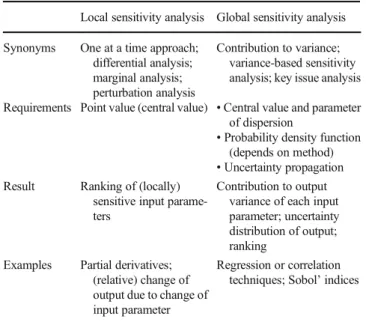
A sensitivity analysis can be performed by varying an input parameter and, as such, determining the effect on the result. Furthermore, if the distribution function of the input parame-ters is known, it is possible to calculate the contribution to the output variance. The first approach belongs to the area of local sensitivity analysis. A local sensitivity analysis determines the effect of a (small) change in one of the input parameters at a time. The second approach belongs to the area of global sen-sitivity analysis. A global sensen-sitivity analysis can be seen as an extension of uncertainty propagation: it determines how much each input parameter contributes to the output variance. While we acknowledge that GSA can be done in several ways, e.g. by density-based methods (Borgonovo and Pliscke2016), we focus in this article on methods that address the contribution to variance (CTV, see Saltelli et al. 2008) and not e.g. on moment-independent methods (as used by Cucurachi2014). The main differences between a local and global sensitivity analysis are illustrated in Table1. In this paper, we focus on global sensitivity analysis, which requires a case study of which the distribution functions of the input parameters are known.
In Fig.1, the procedure of a global sensitivity analysis is illustrated with a schematic LCA model, containing four input parameters. First, the input parameters and their uncertainties are represented by probability density functions (step 1). Second, uncertainty propagation is performed with e.g.
Monte Carlo simulation, which propagates uncertainty through the LCA model (step 2) to obtain a distribution func-tion of the output. Third, the variance of the output is calcu-lated (step 3). After the uncertainty propagation is performed, a method for global sensitivity analysis is selected (step 4), which determines how much each input parameter contributes to the output variance (step 5). In the example of Fig.1, the sensitivity analysis shows that parameter 1 and to a lesser extent parameter 2 are the ones that contribute most to the output variance.
In LCA literature, five methods for global sensitivity anal-ysis have been mentioned that quantify the contribution to output variance: (1) (squared standardized) regression coeffi-cients, as was suggested by Huijbregts et al. (2001) and ap-plied in LCA by e.g. Aktas and Bilec (2012), Basset-Mens et al. (2009), Sugiyama et al. (2005) and Vigne et al. (2012); (2) (squared) Pearson correlation coefficient (Heijungs and Lenzen 2014; Onat et al. 2014); (3) (squared) Spearman (rank) correlation coefficient (Chen and Corson 2014; Geisler et al.2005; Heijungs and Lenzen2014; Mattila et al. 2012; Mattinen et al.2014; Sonnemann et al.2003; Wang and Shen2013); (4) key issue analysis, which applies a first-order Taylor expansion around the LCA model to estimate the out-put variance, thus avoiding sampling; key issue analysis in LCA has been developed by Heijungs (1996) and applied in LCA by e.g. Heijungs et al. (2005) and Jung et al. (2014); and (5) Fourier amplitude sensitivity test has been applied by de Koning et al. (2010).
Outside the LCA domain, a much wider set of approaches have been developed and applied, such as random balance design and the Sobol’method, that also quantify the contribu-tion to output variance (Saltelli et al. 2008; Sobol’ 2001;
Table 1 Main differences between local and global sensitivity analysis, described by differences in input data requirements and results
Local sensitivity analysis Global sensitivity analysis
Synonyms One at a time approach; differential analysis; marginal analysis; perturbation analysis
Contribution to variance; variance-based sensitivity analysis; key issue analysis
Requirements Point value (central value) •Central value and parameter of dispersion
•Probability density function (depends on method)
•Uncertainty propagation Result Ranking of (locally)
sensitive input parame-ters
Contribution to output variance of each input parameter; uncertainty distribution of output; ranking
Examples Partial derivatives; (relative) change of output due to change of input parameter
Tarantola et al.2012; Tarantola et al.2006). The random bal-ance design is closely related to the Fourier amplitude sensi-tivity test, but the sample size does not depend on the number of parameters (Saltelli et al.2008) and is therefore considered to be better suitable for LCA (of which a typical case study contains at least a few hundred input parameters). To our knowledge, random balance design has not yet been applied in LCA. The application of the Sobol’method in LCA has been limited (see for example Wei et al.2014) and for a char-acterization model that can be applied in LCA (Cucurachi 2014). We selected global sensitivity methods that are used most often in LCA (i.e. the squared standardized regression coefficient, squared Spearman (rank) correlation coefficient, key issue analysis). Because these methods were all moment-dependent, we added two moment-dependent methods from outside the LCA field that are currently recommended in the sensitivity analysis field: random balance design (and its cor-responding sensitivity index) and the Sobol’indices (Saltelli et al.2008), which allowed for a quantitative comparison be-tween the selected methods.
For most of the methods, it is not known under which conditions they perform optimally or if there is a method that performs better than the other methods in LCA. The aim of this study is twofold: (1) to study the applicability of a number of previously suggested methods for global sensitivity analysis to LCA, with a focus on the inventory stage, and (2) to compare the methods based on e.g. their ability to explain the output variance. To be able to com-pare the performance of global sensitivity methods, two case studies were constructed: one small hypothetical case study describing electricity production that was sensitive to a small change in the input parameters and a large case
study describing a production system of a northeast Atlantic fishery.
2 Methods for global sensitivity analysis in LCA
2.1 Sampling procedure with matrix-based LCA
In this paper, we use matrix formulation for LCA (for an explanation, see Heijungs and Suh2002). A matrix formula-tion of the LCA model will facilitate the use and discussion of the global sensitivity methods. Matrix-based LCA quantifies the total emissions and resource use (g) of a product over its entire life cycle by:
g¼BA−1f
The production processes are represented byv= 1 toy col-umns in the square technology matrixA(sizex×y); the rows (u= 1 tox) represent a specific product flow. For example, if electricity is produced in one column, other production pro-cesses given in other columns can use it as input. The inven-tory matrix B (sizez×y) consists of use of resources and emissions of (sizew= 1 toz) corresponding to each produc-tion process. Using the final demand vectorf, the production processes are scaled to produce the desired amount. In this paper, we will only consider CO2emissions from each
pro-duction process (soz= 1), transformingBinto a row vectorb
(sizey). The main LCA equations in this paper is therefore:
g¼BA−1f ð1Þ
Step 4:Global sensitivity analysis
Parameter 1
Parameter 2
Parameter 3
LCA model
Step 1:Define input distributions
Step 3: Calculate output distribution
Parameter 4
Parameter 1
Parameter 4
Step 5:Determine contribution to output variance (%)
Parameter 2 Parameter 3
Step 2:
Propagate uncertainty
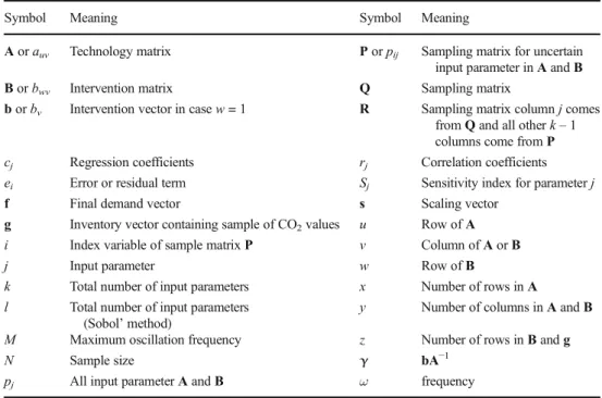
An overview of the symbols introduced in this section can be found in Table2.
Because elements ofAandbwill be uncertain, we devel-oped general formulas based on a row vectorpthat contains all elements ofAandb. Thus,
pvþðu−1Þy¼auv:
and
pxyþv¼bv
We may choose to restrictpto contain uncertain elements ofAandbonly, to save memory. Using this notation, Eq. (1) can be conceived as
g¼γð Þp f
whereγ(p) is a function based on combining the underlying matricesAandb.
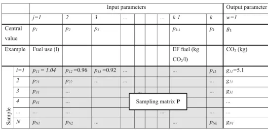
All global sensitivity methods applied in this paper, except for key issue analysis, require sampling for uncertainty prop-agation. In this paper, we used Monte Carlo sampling to gen-erate random numbers and a random balance design to gener-ate equi-distributed numbers, from the distribution functions of the input parameters to generate an output distribution (Fig.2). The sampling matrixP(sizeN×k) containsi =1 to Nrandom numbers drawn for each input parameterj =1 tok of matrixAandb. For example, Monte Carlo sampling could lead to drawing the following random numbers: 1.04, 0.96 and 0.92 for the first three parameters (Fig.2). Combining these values and the realizations for the other parameters in Eq. (1) will lead to the first realization of 5.1 kg CO2(Fig.2). This
procedure is repeatedNtimes; the whole simulation is repeat-ed 50 times.
In this section, six measures, also called sensitivity indices, that quantify the contribution to output variance are intro-duced. The mathematical notations in the case of matrix-based LCA are given; the full derivation can be found in the Electronic Supplementary Material. All sensitivity methods a r e p r o g r a m m e d i n M a t L a b a n d a r e a v a i l a b l e a t evelynegroen.github.io.
Calculating sensitivity indices, there are four aspects that can differ per method. The comparison of the sensitivity methods will be based on these four aspects:
I. The sampling design (i.e. how the rows of P are constructed)
II. The total output variance
III. The total output variance (II) that is explained by the method (this is ideally 100%)
IV. The contribution to (III) of the individual input parameters
The relation between the output variance (II), explained variance (III) and the contribution to variance (IV) is visual-ized in Fig.3.
In general, the variance of the model output in Eq. (1) is given by the conditional variance of parameterpjand a resid-ual term (or error term):
varð Þ ¼g var E gjpj
þE var gjpj
ð2Þ
The conditional variance var(E(g|pj)) is theBexpected re-duction in variance that would be obtained if parameter
Table 2 Meaning of symbols
Symbol Meaning Symbol Meaning
Aorauv Technology matrix Porpij Sampling matrix for uncertain
input parameter inAandB Borbwv Intervention matrix Q Sampling matrix
borbv Intervention vector in casew= 1 R Sampling matrix columnjcomes
fromQand all otherk–1 columns come fromP
cj Regression coefficients rj Correlation coefficients
ei Error or residual term Sj Sensitivity index for parameterj
f Final demand vector s Scaling vector
g Inventory vector containing sample of CO2values u Row ofA i Index variable of sample matrixP v Column ofAorB
j Input parameter w Row ofB
k Total number of input parameters x Number of rows inA
l Total number of input parameters (Sobol’method)
y Number of columns inAandB
M Maximum oscillation frequency z Number of rows inBandg
N Sample size γ bA−1
pjcould be fixed^(Saltelli et al.2010).Eis the expected value, and varð Þ ¼g 1
N−1∑iðgi−gÞ 2 and g¼N1∑igi. The variance
explained by each of the parameter can be given by the cor-relation ratio (McKay et al. 1999; Saltelli et al. 2008, Eq. (1.25)):
Sj¼
var E gjpj
varð Þg ð3Þ
where the ratioSjis the (main) sensitivity index. A derivation of the sensitivity index can be found in the Electronic Supplementary Material (I), Eqs. (A.1) to (A.4). The expres-sions for the sensitivity indices for each method are found in the boxed equations in the next subsections.
2.2 Regression- or correlation-based methods for sensitivity analysis
The contribution to variance can be quantified using sion or correlation. First, the general framework of a regres-sion model is introduced. According to the theory of multiple linear regressions,gcan be described by
gi¼c0þ∑kj¼1cjpijþei ð4Þ
where the constantc0represents the intercept,cjthe slope (or regression coefficient) andeithe error term, which is assumed to be normally distributed with a constant variance. The
sensitivity index using the squared standardized regression coefficients (SRCs) is equal to
SSRCj ¼ ∑
i pij−pj
gi−g
2
∑ i
pij−pj
2
∑i gi−g
2 ¼
var pj
varð Þg cj 2
ð5Þ
where var pj ¼ 1
N−1∑i pij−pj
2 and p
j¼N1∑ipij. The
full description of Eq. (5) is given in the Electronic Supplementary Material (II) in Eqs. (A.5)–(A.9).
The SSRCj , similar to the Pearson correlation coefficient squared, is not robust to outliers (Hamby1994; Saltelli and Sobol1995). An alternative to the Pearson correlation coeffi-cient is using its rank-transformed counterpart, in the form of the Spearman rank correlation coefficient. The squared Spearman correlation coefficient (SCC) calculates the linear dependence between the input and output parameters. Each draw of input parameterpijis rank-transformed top(i)j, andgi is rank-transformed tog(i). The Spearman correlation
coeffi-cient is calculated as follows:
rSCCj ¼ ∑
i
pð Þij−pj
gð Þi−g
ffiffiffiffiffiffiffiffiffiffiffiffiffiffiffiffiffiffiffiffiffiffiffiffiffiffiffiffiffiffiffiffiffiffiffiffiffiffiffiffiffiffiffiffiffiffiffiffiffiffiffi
∑i pð Þij−pj
2
∑i gð Þi−g
2
r ð6Þ
s r e t e m a r a p t u p n
I Output parameter
j=1 2 3 ... ... k-1 k w=1
Central
value
p1 p2 p3 pk-1 pk
Example Fuel use (l) EF fuel (kg
CO2/l)
CO2 (kg)
Sam
ple
i=1 p11 = 1.04 p12 =0.96 p13 =0.92 ... ... p1k g11=5.1
2 p21 p22 ... ... ... g21
3 p31 ... ... ... g31
4 p41 ... ...
... ... ... ... ... ...
N pN1 pN2 ... ... pNk gN1
Sampling matrix P
Fig. 2 Monte Carlo sampling approach for matrix-based calcu-lations in LCA.EFemission factor
Total output variance (II)
m r e t l a u d i s e R ) I I I ( e c n a i r a v t u p t u o d e n i a l p x E
Contribution to variance by input parameters (IV)
S1 S2 S3 ... ... Sk-1 Sk
The sensitivity index using SCC is equal to
SSCCj ¼ rSCCj
2
ð7Þ
The full description of Eq. (7) is given in the Electronic Supplementary Material in (A.10). In this paper, sensitivity
indices based on SRC SSRCj
and SCC SSCCj
are
calculat-ed from the same simulations.
2.3 Key issue analysis using a first-order Taylor expansion
Key issue analysis (KIA) is a method for analytically deter-mining the contribution to variance (or variance decomposi-tion) by means of a order Taylor expansion. The first-order Taylor expansion around the central values (pj ) of Eq. (1) results in
gj¼g pj ¼g pj þ ∂g pj ∂pj
0 @
1 A pj−pj
ð8Þ
Because the total output variance var(g) is estimated by the first-order Taylor expansion, the variance explained by the individual parameters will always be equal to 100% (Fig.3). The variance according to KIA, therefore, may be of a differ-ent magnitude than the output variance obtained by sampling. The sensitivity index using KIA is equal to
SKIAj ¼ var pj
varð Þg ∂g ∂pj
!2
ð9Þ
The full derivation of Eq. (9) is given in the Electronic Supplementary Material (III), in Eqs. (A.11)–(A.13).
2.4 Variance-based methods for sensitivity analysis
2.4.1 Sobol’indices
In the case of variance-based methods for sensitivity analysis, the variance of Eq. (1) is rewritten as the sum of the variance of all first-order conditional variances and higher-order terms (Electronic Supplementary MaterialIV, Eqs. (A.14)–(A.15)):
varð Þ ¼g ∑jvar E gjpj
þ∑l∑j>l
var E gjpj;pl
−var E gjpj
−varðE gð jplÞÞ
þ…
ð10Þ
To calculate the conditional variances of Eq. (3), we have adopted the sampling algorithm described by (Saltelli et al. 2010). The sampling algorithm fixes one parameter to calcu-late the variance reduction in the output. The sampling
algorithm requires two sampling matrices. In addition to the sampling matrixP, a second sampling matrixQis generated in the same way, independent ofP. FromPandQ, a third sam-pling matrix is derivedR, from which columnjcomes fromQ
and all otherk−1 columns come fromP. For each matrixP,Q
and R, the output of the model is calculated using Eq. (1), resulting ing(P),g(Q) andg(R). The variance is calculated through the identity var(g) =E(g2)−E2(g). The variance equals
varð Þ ¼g 1
N∑i gð ÞP i
2
− 1
N∑igð ÞP i
2
ð11Þ
Likewise, the conditional variance is given by
var E gjpj
¼ 1
N∑igð ÞQ g R j
i−gð ÞP i
ð12Þ
The sensitivity index, applying Sobol’s main effect (SME) index (Electronic Supplementary MaterialIV, Eq. (A.17)), is equal to
SSM Ej ¼ 1
N P
igð ÞQ gð ÞRj i−gð ÞP i
1
N P
i gð ÞP i
2
− 1
N P
igð ÞP i
2 ð13Þ
The Sobol’total effect index (STE) calculates how much input parameterjexplains of the output variance, including all possible interactions with other parameters:
SSTEj ¼SjþSjlþSjmþ…þSjlmþ…Sjlm…k ð14Þ
The total effect index equals the Bexpected variance that would be left if all [parameters] but [parameterpj] could be fixed^(Saltelli et al.2010) and is based on the quantification of the residual term in Eq. (2):
E var gjp∼j
¼ 1
2N∑i gð ÞP i−g R j
i
2
ð15Þ
wherep~jrefers to fixing all parameters except for parameterj. The Sobol’ total effect index (Electronic Supplementary MaterialIV, Eq. (A.19)) is equal to
SSTEj ¼ 1
2N∑i gð ÞP i−g R j
i
2
1
N∑i gð ÞP i
2
− 1
N∑igð ÞP i
2 ð16Þ
In the case of an LCA model that behaves approximately linear, all interaction terms (e.g. Sjl and other higher-order terms in Eq. (14)) are approximately zero, soSSTE
j ≈SSMEj , in
could be seen as a non-linear effect) or interaction terms can be larger than 100% (Electronic Supplementary MaterialIV, Eq. (A.20)–(A.21)).
2.4.2 Random balance design
The theory of Fourier series states that any (periodic) function can be written as a sum of wave functions. Random balance designs (RBDs) calculate the conditional variance by rewrit-ing the LCA model in Eq. (1) in terms of sums of sine and cosine functions. We use complex numbers to facilitate nota-tion of sine and cosine, thus usingepffiffiffiffi−1ω, where we prefer to writepffiffiffiffiffiffi−1 overi, allowing us to remain usingias an index variable. For this method, we use the discrete Fourier trans-formation to convert an equally spaced periodic function of sizeN. The model output of Eq. (1) in terms of Fourier coef-ficients are given in the Electronic Supplementary Material (V), Eq. (A.24). The Fourier coefficients are given by
g pð Þ ¼ω 1 N∑
N−1
i¼0g pij e− ffiffiffiffi −1 p
πωi=N ð17Þ
where omega (ω) represents the frequency domain, which is divided in equally spaced segments:ω= 1 toN−1. The pa-rameters that contribute most to the output variance will re-semble the wave-like shape of the input parameter. This means that the most sensitive parameters have the highest amplitude and that the amplitude of the wave of the output is a measure of the conditional variance of input parameterj. The total variance is given by
varð Þ ¼g 1 N∑
N−1
ω¼1jg pð Þω j
2
ð18Þ
A similar expression is found for the conditional variance of each input parameter (Eq. A.28). The sensitivity index using RBD is equal to
SRBDj ¼2 ∑ M
ω¼1jgjð Þpω j
2
∑N−1
ω¼1jg pð Þω j
2 ð19Þ
whereMis equal to the maximum oscillation frequency and gj(pω) is the reordered model output for parameter j. The derivation of the sensitivity index in Eq. (19) can be found in the Electronic Supplementary Material (V) and in Xu and Gertner (2011).
2.5 Case studies
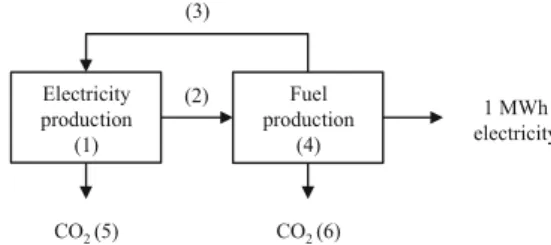
A hypothetical case study describing the production of 1 MWh of electricity was selected (the original version of the case study appeared in Heijungs and Suh2002). The case study consisted of two processes: fuel production and
electricity production (Fig.4). In Fig.4, parameter 1 equals the electricity production, parameter 2 equals fuel use for elec-tricity production, parameter 3 equals elecelec-tricity use of fuel production, parameter 4 equals fuel production, parameter 5 equals CO2emissions during fuel production and parameter 6
equals CO2emissions during electricity production. The case
study is set up in such a way that a small change in one of the input parameters results in a large change of the output.
We assumed that the input parameters were log-normally distributed and the relative standard deviation (i.e. coefficient of variation:cv= σ/μ) equalled 5 or 30% for two different scenarios. All input parameters are assumed log-normally dis-tributed to avoid drawing random numbers with an incorrect sign. This is admittedly a weak argument, but our main pur-pose is to construct a toy example to study the sensitivity indices, not to build a realistic system. We selected a relative small and large coefficient of variation because we wanted to explore if the Sobol’total sensitivity indices and the Spearman correlation coefficients would explain more of the output var-iation in case of outliers.
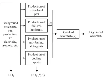
The second case study describes a whitefish fishery in the northeast Atlantic. The functional unit equalled 1 kg landed whitefish. A flow diagram is shown in Fig. 5. Five input parameters we wish to highlight are as follows: parameterα, total amount of landed fish; parameterβ, emission factor fuel combustion; parameterγ, fuel production; parameterδ, emis-sion factor fuel production and parameter ε, fuel use. The fishery consists of a single vessel, making trips of approxi-mately 2 weeks, landing their fish in Tromsø, Norway. Data comprised annual averages of the vessel and gear, fuel, lubri-cants, anti-fouling, detergents, cooling agents and total catch and were collected by the vessel owner. Background data, such as the CO2emissions during steel production from the
vessel, came from the ecoinvent database v2.2 (ecoinvent 2007). In total, 115 input parameters were considered. Also, in this case study, we assumed that all input parameters were log-normally distributed with acvof 5 or 30%.
3 Results
In this section, we will discuss the sampling design (I), total output variance (II), the explained variance (III) and the
Electricity production
(1)
CO2 (5) CO2 (6)
Fuel production
(4)
1 MWh electricity (2)
(3)
contribution to the output variance of the individual input parameters as given by the sensitivity indicesSj(IV).
3.1 Sampling design
The differences in uncertainty propagation methods require differences in sample designs and, therefore, in computational effort between methods (Table3). SRC, SCC and RBD both requireNruns, but for the Sobol’indices (SME and STE) 2N runs are needed to calculate the indices. This means that this method is more computationally demanding than the other sampling methods. Although KIA requires only a single cal-culation, it does not produce a distribution function of the output, making it more difficult to compare two or more stud-ies. RBD is using the discrete Fourier series, which allowed us to use the fast Fourier transformationalgorithm, which is computationally fast (Frigo and Johnson2005).
3.2 Output variance and explained variance
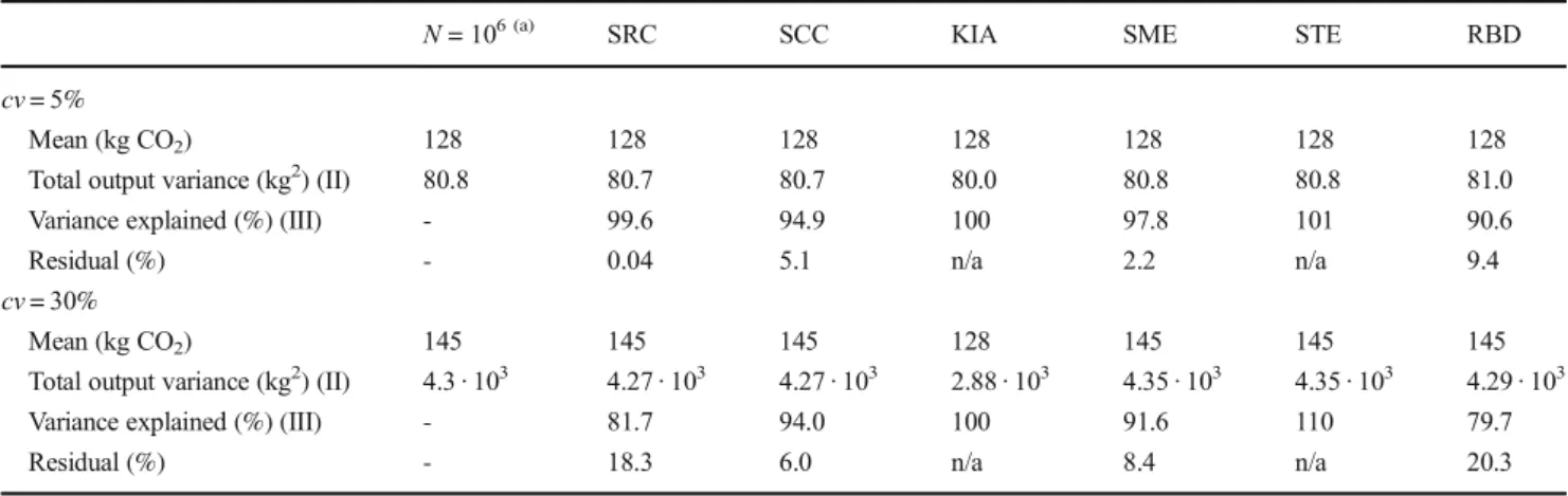
Table4shows the mean, total output variance (II) and vari-ance explained by the global sensitivity method (III) of case study 1, in the case of a parameter of dispersion ofcv= 5% andcv= 30%, for a sample size ofN =4096 and 50 repeti-tions. The sample size was chosen to align with Groen et al.
(2014). In order to make a proper comparison, we ran an additional Monte Carlo simulation where we calculated the output variance based onN= 106, and we considered this as the best approximation of the output variance.
Forcv= 5%, all methods produced approximately the same mean and output variance for this case study. Variance ex-plained by most methods added up to approximately 100%, suggesting a linear behaviour. Forcv= 30%, most methods produced approximately the same mean and output variance. However, KIA estimated the total output variance consider-ably lower than the sampling-based methods. Furthermore, SRC explained less than SCC, which suggested the presence of outliers. STE also showed a value much larger than 100%, which also suggested the presence of outliers. RBD explained less of the output variance than other methods. Note that the mean value for CO2is larger when thecvis larger, although
the mean value of the input parameters is the same. This is an effect of the asymmetric distribution used. KIA neglects the shape of the distribution and therefore misses this effect.
Table 5 shows the mean and the output variance (II) for case study 2 in the case of a parameter of dispersion ofcv= 5% and cv = 30%. Case study 2 contains 115 parameters; the variance explained (III) is shown of the 5 most contributing parameters and for all 115 parameters, because all other pa-rameters contribute <<1%.
Forcv= 5%, all methods produced approximately the same mean and output variance. Most methods explained approxi-mately 100% of the variance, suggesting a linear behaviour. Forcv = 30%, most methods produced approximately the same mean and output variance, except for KIA. KIA estimat-ed the total output variance considerably lower than the sampling-based method. In the case of RBD, the output ex-plained by 5 or by 115 parameters differed considerably, sug-gesting that RBD overestimated the sensitivity indices of low contributing parameters.
3.3 Sensitivity index
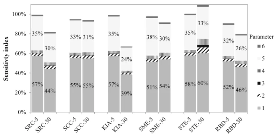
Figure6shows the sensitivity index (IV) of each parameter of case study 1 for a parameter of dispersion of cv= 5% and cv= 30%, scaled to the benchmark output variance computed
Production of vessel and
gear
Catch of whitefish (α) Production of
fuel (γ), lubricants
Production of anti-fouling,
detergents Background
processes, e.g. production
of electricity, iron ore, etc.
Production of cooling
agents
1 kg landed whitefish
CO2 CO2 (δ; β)
(ε)
Fig. 5 Case study 2: production of 1 kg of landed whitefish from the northeast Atlantic (Groen et al.2014)
Table 3 Sample design and calculation of the output variance for the six sensitivity indices
Methods Uncertainty propagation Sampling design (I) Runs
Standardized regression coefficient Sampling Random N Spearman correlation coefficient Sampling Random N
Key issue analysis Analytical N/A 1
Sobol’main effect Sampling 2× random 2N
Sobol’total effect Sampling 2× random 2N
Random balance design Stratified sampling Wave-like, equally distributed and of size 2N
withN= 106. We scaled the graphs to this benchmark to com-pensate for methods that predicted a lower output variance. For example, for acvof 30%, KIA arrived at an output variance of 0.606, which is approximately 20% lower than the output var-iance with a sample size ofN= 106. In the case of applying SRC to case study 1 (cv= 5 %), parameter 1 was responsible for 57% of the output variance. For each method, parameters 1 and 5 contributed most to the output variance; the exact contri-bution, however, differed per method. Parameters 2, 4 and 6 each have a contribution of approximately 1–6%; parameter 3 contributed less than 0.7% to the output variance. There are
some differences in the ranking of parameters 2, 4 and 6 be-tween the various methods.
Figure 7 shows the sensitivity index (III) of the five most dominant parameters in the case of a parameter of dispersion of cv = 5% and cv = 30%. The sensitivity indices (III) are shown only for the five most contributing parameters, because all other parameters contribute <<1%. Although for each method, parameters α and β contribut-ed most to the output variance, the exact contribution differed per method. All methods agreed on the much smaller contribution (around 1%) of parameters γ, δ and
Table 4 Mean and variance of LCA model output for different sensitivity methods for case study 1 (N= 4096; 50 repetitions), using squared standardized regression coefficients (SRC), squared Spearman correlation coefficients (SCC), key issue analysis (KIA), Sobol’main effect (SME), Sobol’total effect (STE), and random balance design (RBD)
N= 106 (a) SRC SCC KIA SME STE RBD
cv= 5%
Mean (kg CO2) 128 128 128 128 128 128 128
Total output variance (kg2) (II) 80.8 80.7 80.7 80.0 80.8 80.8 81.0
Variance explained (%) (III) - 99.6 94.9 100 97.8 101 90.6
Residual (%) - 0.04 5.1 n/a 2.2 n/a 9.4
cv= 30%
Mean (kg CO2) 145 145 145 128 145 145 145
Total output variance (kg2) (II) 4.3 · 103 4.27 · 103 4.27 · 103 2.88 · 103 4.35 · 103 4.35 · 103 4.29 · 103
Variance explained (%) (III) - 81.7 94.0 100 91.6 110 79.7
Residual (%) - 18.3 6.0 n/a 8.4 n/a 20.3
(a)
The best approximation of the output mean and variance is evaluated at a sample size of N = 106
Table 5 Mean, output variance and variance explained by 5 or 115 parameters of LCA model output for different sensitivity methods for case study 2 (N= 4096; 50 repetitions), using squared standardized regression coefficients (SRC), squared Spearman correlation coefficients (SCC), key issue analysis (KIA), Sobol’main effect (SME), Sobol’ total effect (STE), and random balance design (RBD)
N = 106 (a) SRC SCC KIA SME STE RBD cv= 5%
Mean (kg CO2) 1.96 1.96 1.96 1.95 1.96 1.96 1.96 Total output variance
(kg2) (II) 0.0170 0.0170 0.0170 0.0168 0.0169 0.0169 0.0170 Variance explained(c)
(%) (III) - 5
- 99.2% 95.4% 100% 95.1% 101% 90.2%
Variance explained(d) (%) (III) - 115
- 99.2% 95.5% 100% 95.2% 101% 101%
Residual (%) - 0.8% 4.5% n/a 4.8% n/a und.(b)
cv= 30%
Mean (kg CO2) 2.16 2.16 2.16 1.95 2.16 2.16 2.16 Total output variance
(kg2) (II)
0.76 0.758 0.758 0.606 0.775 0.775 0.766
Variance explained(c) (%) (III) - 5
- 87.2 94.4 100 93.6 103 83.3
Variance explained(d) (%) (III) - 115
- 87.3 94.5 100 93.6 103 94.0
Residual (%) - 12.7 5.5 n/a 6.4 n/a 6.0
(a)The best approximation of the output mean and variance is evaluated at a sample size of N = 106 (b)
und: undefined: because the explained variance was more than 100% due to an overestimation of the sensitivity indices of the low contributing parameters, the residual could not be defined.
(c)
Variance explained by the five most contributing parameters. (d)
ε, although there are differences in the precise value, as well as in the ranking.
4 Discussion
Table6gives an indication of performance of the sensitivity methods,averaged overthe two case studies, under conditions of small (cv= 5%) and large input uncertainties (cv= 30%). The evaluation of the sampling design (I) relates to the com-putational effort of a sensitivity method: KIA does not make use of sampling and was fastest. RBD was faster than SRC and SCC due to the implementation of the fast Fourier transformationalgorithm. SME and STE have to generate two sampling matrices and, therefore, were slowest. The eval-uation of the sampling design (I) was as follows: (++)
independent on the sample size N; (+) using an optimized sample algorithm; (−) dependent on N and (−) dependent on (2× N).
The total output variance (II) calculated with each method resulted in approximately the same output variance, except for KIA, which underestimated the output variance especially in the case of high input uncertainties. The evaluation of the output variance was as follows: (++) equalled on average 99–101% of the output variance (compared to the output var-iance calculated with a sample size ofN = 106, which was assumed to be the best estimate); (+) equalled ≥95%; (−) equalled ≥90% and (−) equalled <90% of the best estimate of the output variance.
The variance that is explained by each method (III) is equal to the sum of the sensitivity coefficients (IV). The evaluation of the main sensitivity indices (all indices except STE) was as follows: (++) explained on average 99–101% of the output
57%
44% 55% 55%
57% 39%
51% 54% 58% 60% 52%46%
35%
30%
33% 31% 35%
24%
38% 30% 35%
33%
32% 26%
0% 20% 40% 60% 80% 100%
Sensitivty index
Parameter
6
5
4
3
2
1
Fig. 6 Contribution to output variance for sensitivity methods applied to case study 1 (N= 4096; 50 repetitions;cv= 5% orcv= 30%) for the sensitivity index (SRC, SCC, KIA, SME, RBD) or total sensitivity index (STE) for each parameter (1–6) is shown.SRC squared standardized regression coefficient;SCCsquared Spearman correlation coefficient;
KIAkey issue analysis;SMESobol’main effect index;STESobol’total effect index;RBDrandom balance design;1electricity production;2fuel use electricity production;3electricity use fuel production;4fuel produc-tion; 5CO2 emission fuel production;6 CO2emission electricity production
40%
38%
38% 37% 41%
32%
40% 37% 41% 41% 37%
33%
0% 20% 40% 60% 80% 100%
Sensitivty index
Parameter
ε
δ
γ
β
α 56%
46% 54% 55% 56%45% 52% 53%
57% 58%
51% 47%
Fig. 7 Contribution to output variance for sensitivity methods applied to study 2 (N= 4096; 50 repetitions;cv= 5% orcv= 30%) for the sensitivity index (SRC, SCC, KIA, SME, RBD) or total sensitivity index (STE) for each parameter (α–ε) is shown.SRCsquared standardized regression coefficient;SCCsquared Spearman correlation coefficient;KIAkey issue
variance (compared the output variance calculated for each method); (+) explained≥95%; (−) explained≥90% and (−) explained <90% of the output variance. The evaluation of the total sensitivity index (STE) is given by the difference with SME. If STE is equal to SME, there is no use for calculating STE: the bigger the difference between the two indices, the more relevant it becomes to calculate the following: (++) STE− SME≥10%; (+) STE− SME≥5%; (−) STE−SME <5 % and (−) STE≈SME.
There were some limitations to the case studies that were used to evaluate the sensitivity methods. First, all parameters are assumed to be uncorrelated, which is a simplification be-cause of lack of data. When correlations are present, including correlated inputs will increase the accuracy of the outcome of the global sensitivity analysis (Jacques et al.2006; Xu and Gertner2008b). A global sensitivity index given by SRC for models with correlated inputs can be found in Xu and Gertner (2008b), given by the Sobol’indices in Jacques et al. (2006) and given by the RBD and its corresponding indices in Xu and Gertner (2008a).
Second, the performance indicators in Table6are based on two case studies with two different sets of input parameters, which is limited. Other types of distribution functions or case studies with more interacting input parameters, for example, were not considered. However, we assumed that not so much the type of distribution function will influence the set of rec-ommended methods, but that it primarily relies on the first moment of the input uncertainty (increasing the chance of outliers and the effect of interactions leading to non-linear behaviour) (Saltelli et al.2008).
Third, we only considered the inventory stage in this paper. Usually, an LCA includes a midpoint or even an endpoint assessment. In general, the midpoint to inventory calculation step is assumed to be linear, but the inventory to midpoint or midpoint to endpoint relations could be non-linear; in these cases, the Sobol’ method might be preferred because it is better able to include non-linear effects (Iooss and Lemaître 2014; Sobol’ 2001). An illustrative example is given in Cucurachi (2014), where sensitivity indices were quantified
in the case of impact assessment of noise on human health, resulting in high values for STE compared to SME, illustrat-ing the benefit of usillustrat-ing Sobol’indices as a measure of global sensitivity.
Fourth, this article started from moment-based approaches, in particular the contribution to variance. An extension of our analysis to moment-independent approaches seems to be a logical next step.
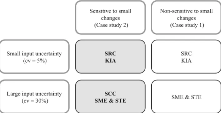
Figure8gives an overview of the best performing methods in the case of large (cv= 30 %) or small (cv= 5 %) input uncertainty and a situation beingBsensitive^(case study 1) or Bnon-sensitive^(case study 2) to small changes of the input parameters, where Bsensitive^ means that a small relative change of an input parameter may produce a large relative change of an output variable. Although our LCA model con-tains a matrix inverse and is therefore non-linear in its param-eters and could potentially be sensitive in this sense (Heijungs 2002), only the first case study displayed sensitivity to small changes. Figure8is based on evaluating Tables4and5 sim-ilar to how we reached Table6, but keeping the result of case studies 1 and 2 separate to make a distinction between the sensitive and non-sensitive case studies. The results of the evaluation per case study can be found in the Electronic Supplementary Material (VI). The computational effort was not taken into account in this evaluation, since this indicator
Table 6 Performance of the sensitivity methods averaged over the two case studies on a scale from poor (−), insufficient (−), sufficient (+) to good (++)
SRC SCC KIA SME STE RBD
Sample design (I)—computational effort − − ++ − − + Ability to calculate total output variance (II):
•Small input uncertainties (cv =5 %) ++ ++ ++ ++ ++ ++
•Large input uncertainties (cv =30 %) ++ ++ − + + ++ Ability to explain output variance (III) and calculate sensitivity indices (IV):
•Small input uncertainties (cv =5 %) ++ + ++ + + −
•Large input uncertainties (cv =30 %) − − ++ − ++ −
A detailed description of the scales is found in the text
SRCsquared standardized regression coefficient,SCCsquared Spearman correlation coefficient,KIAkey issue analysis,SMESobol’main effect index,STESobol’total effect index,RBDrandom balance design
Sensitive to small changes (Case study 2)
Non-sensitive to small changes (Case study 1)
Small input uncertainty (cv = 5%)
Large input uncertainty (cv = 30%)
SRC KIA
SRC KIA
SCC
SME & STE SME & STE
seemed less relevant as even the slowest performing methods took less than an hour. Both performance indicators (II: ability to quantify the output variance) and (III: ability to explain the output variance) weighted equally.
When restricted to the assumptions that LCAs are behaved linearly up to the midpoint assessments, the sensitivity indices using SRC or KIA (when input uncertainties are relatively small) or sensitivity indices derived by SCC or the Sobol’ indices (when input uncertainties are large) could be used for global sensitivity analysis (Fig.8). However, the choice for a global sensitivity method also depends on (1) data avail-ability to the LCA practitioner and (2) the aim of the study. Regarding data availability, if only a parameter of dispersion could be defined and not a probability distribution function, applying KIA is a feasible option, especially when input un-certainties are small, since a distribution function is not re-quired. If probability distribution functions are provided, methods using KIA or SRC (low input uncertainties) and SCC or SME/STE (large input uncertainties) are most feasi-ble. Using Monte Carlo simulation to propagate uncertainty to calculate the sensitivity indices, both SRC and SCC could be calculated as well using the same sample. Likewise, SME and STE are calculated from the same dataset, which could be another reason for selecting the preferred sensitivity analysis method.
Regarding the aim of the study, we will give three exam-ples. First, a goal of an LCA can be to determine whether there is a significant difference between two (or more) scenarios. In that case, sampling-based global sensitivity methods such as SRC or SME can determine which input parameters contrib-ute most to the output variance and therefore should be known most accurately before propagating their uncertainty through the LCA model.
Second, if the goal of an LCA is to assess the performance of a single production system, depending on the nature of the input uncertainties, methods such as KIA but also sampling-based methods such as SCC can help to indicate parameters that could contain opportunities for improvement regarding environmental performance (Heijungs1994). Third, when re-peating an LCA of similar goal and scope, the input parame-ters that contribute only minor to the output variance accord-ing to either of the methods mentioned in Fig.8can set to a fixed value to simplify (future) data collection.
5 Conclusions
The aim of this study was twofold: (1) to study the applicabil-ity of a number of previously suggested methods for global sensitivity analysis to LCA and (2) to compare the methods based on their ability to explain the output variance, using a number of case studies. Five methods that quantify the contri-bution to output variance were evaluated: squared
standardized regression coefficient (SRC), squared Spearman correlation coefficient (SCC), key issue analysis (KIA), Sobol’indices (STE and SME) and random balance design index (RBD). Most methods performed approximately equally well for quantifying output variance and contribution to variance of the input parameters, especially for relatively small input uncertainties. In the case of large input uncer-tainties, methods robust to outliers such as squared Spearman correlation coefficient or the Sobol’indices per-formed better than the other methods.
When restricted to the assumptions that quantification of environmental impact in LCAs behaves linearly, squared stan-dardized regression coefficients, squared Spearman correla-tion coefficients, the Sobol’indices or key issue analysis can be used for global sensitivity analysis. The choice for one of the methods depends on the available data, the magnitude of the uncertainties of the data and the aim of the study.
Acknowledgements Data and funding was provided by the Seventh Framework Programme (FP7) EU project BWhiteFish^ (www.whitefishproject.org), a research project to the benefit of small and medium enterprise associations, grant agreement no 286141.
Open AccessThis article is distributed under the terms of the Creative C o m m o n s A t t r i b u t i o n 4 . 0 I n t e r n a t i o n a l L i c e n s e ( h t t p : / / creativecommons.org/licenses/by/4.0/), which permits unrestricted use, distribution, and reproduction in any medium, provided you give appropriate credit to the original author(s) and the source, provide a link to the Creative Commons license, and indicate if changes were made.
References
Aktas CB, Bilec MM (2012) Impact of lifetime on US residential building LCA results. Int J Life Cycle Assess 17:337–349
Basset-Mens C, Kelliher F, Ledgard S, Cox N (2009) Uncertainty of global warming potential for milk production on a New Zealand farm and implications for decision making. Int J Life Cycle Assess 14:630–638
Borgonovo E, Pliscke E (2016) Sensitivity analysis: a review of recent advances. Eur J Oper Res 248:869–887
Chen X, Corson MS (2014) Influence of emission-factor uncertainty and farm-characteristic variability in LCA estimates of environmental impacts of French dairy farms. J Clean Prod 81:150–157
Clavreul J, Guyonnet D, Tonini D, Christensen T (2013) Stochastic and epistemic uncertainty propagation in LCA. Int J Life Cycle Assess 18:1393–1403
Cucurachi S (2014) Impact assessment modelling of matter-less stressors in the context of Life Cycle Assessment. PhD Thesis, Leiden University
de Koning A, Schowanek D, Dewaele J, Weisbrod A, Guinée J (2010) Uncertainties in a carbon footprint model for detergents; quantifying the confidence in a comparative result. Int J Life Cycle Assess 15: 79–89
ecoinvent (2007) Centre e Swiss Centre for Life Cycle Inventories. www.ecoinvent.org
Geisler G, Hellweg S, Hungerbühler K (2005) Uncertainty analysis in life cycle assessment (LCA): case study on plant-protection products and implications for decision making. Int J Life Cycle Assess 10: 184–192
Groen EA, Heijungs R, Bokkers EAM, de Boer IJM (2014) Methods for uncertainty propagation in life cycle assessment. Environ Model Soft 62:316–325
Hamby DM (1994) A review of techniques for parameter sensitivity anal-ysis of environmental models. Environ Monit Assess 32:135–154 Heijungs R (1994) A generic method for the identification of options for
cleaner products. Ecol Econ 10:69–81
Heijungs R (1996) Identification of key issues for further investigation in improving the reliability of life-cycle assessments. J Clean Prod 4: 159–166
Heijungs R (2002) The use of matrix perturbation theory for addressing sensitivity and uncertainty issues in LCA. p. 77–80. In: Anonymous (ed) Proceedings of the fifth international conference on ecobalance. Practical tools and thoughtful principles for sustainability. Nov. 6– Nov. 8, 2002, Epochal Tsukuba, Tsukuba, Japan
Heijungs R, Lenzen M (2014) Error propagation methods for LCA—a comparison. Int J Life Cycle Assess 19:1445–1461
Heijungs R, Suh S (2002) The computational structure of life cycle as-sessment. Kluwer Academic Publishers, Dordrecht
Heijungs R, Suh S, Kleijn R (2005) Numerical approaches to life cycle interpretation—the case of the Ecoinvent’96 database. Int J Life Cycle Assess 10:103–112
Huijbregts MJ et al (2001) Framework for modelling data uncertainty in life cycle inventories. Int J Life Cycle Assess 6:127–132
Iooss B, Lemaître P (2014) A review on global sensitivity analysis methods. arXiv preprint arXiv:14042405
Jacques J, Lavergne C, Devictor N (2006) Sensitivity analysis in presence of model uncertainty and correlated inputs. Reliab Eng Syst Safe 91: 1126–1134
Jung J, von der Assen N, Bardow A (2014) Sensitivity coefficient-based uncertainty analysis for multi-functionality in LCA. Int J Life Cycle Assess 19:661–676
Lloyd SM, Ries R (2007) Characterizing, propagating, and analyzing uncertainty in life-cycle assessment: a survey of quantitative ap-proaches. J Ind Ecol 11:161–179
Mattila T, Leskinen P, Soimakallio S, Sironen S (2012) Uncertainty in environmentally conscious decision making: beer or wine? Int J Life Cycle Assess 17:696–705
Mattinen MK, Heljo J, Vihola J, Kurvinen A, Lehtoranta S, Nissinen A (2014) Modeling and visualization of residential sector energy con-sumption and greenhouse gas emissions. J Clean Prod 81:70–80 McKay MD, Morrison JD, Upton SC (1999) Evaluating prediction
un-certainty in simulation models. Comput Phys Commun 117:44–51 Mutel CL, de Baan L, Hellweg S (2013) Two-step sensitivity testing of
parametrized and regionalized life cycle assessments: methodology and case study. Environ Sci Technol 47:5660–5667
Onat N, Kucukvar M, Tatari O (2014) Integrating triple bottom line input–output analysis into life cycle sustainability assessment framework: the case for US buildings. Int J Life Cycle Assess 19:1488–1505
Saltelli A, Sobol IM (1995) About the use of rank transformation in sensi-tivity analysis of model output. Reliab Eng Syst Saf 50:225–239 Saltelli A, Tarantola S, Chan KPS (1999) A quantitative
model-independent method for global sensitivity analysis of model output. Technometrics 41:39–56
Saltelli A et al. (2008) Introduction to sensitivity aalysis. In: Global sen-sitivity analysis. The Primer. Wiley, Ltd, pp 1–51
Saltelli A, Annoni P, Azzini I, Campolongo F, Ratto M, Tarantola S (2010) Variance based sensitivity analysis of model output. Design and estimator for the total sensitivity index. Comput Phys Commun 181:259–270
Sobol’IM (2001) Global sensitivity indices for nonlinear mathematical models and their Monte Carlo estimates. Math Comput Simulat 55: 271–280
Sonnemann GW, Schuhmacher M, Castells F (2003) Uncertainty assess-ment by a Monte Carlo simulation in a life cycle inventory of elec-tricity produced by a waste incinerator. J Clean Prod 11:279–292 Sugiyama H, Fukushima Y, Hirao M, Hellweg S, Hungerbühler K (2005)
Using standard statistics to consider uncertainty in industry-based life cycle inventory databases. Int J Life Cycle Assess 10:399–405 Tarantola S, Gatelli D, Mara TA (2006) Random balance designs for the estimation of first order global sensitivity indices. Reliab Eng Syst Safe 91:717–727
Tarantola S, Becker W, Zeitz D (2012) A comparison of two sampling methods for global sensitivity analysis. Comput Phys Commun 183: 1061–1072
Vigne M, Martin O, Faverdin P, Peyraud J-L (2012) Comparative uncer-tainty analysis of energy coefficients in energy analysis of dairy farms from two French territories. J Clean Prod 37:185–191 Wang E, Shen Z (2013) A hybrid data quality indicator and statistical
method for improving uncertainty analysis in LCA of complex sys-tem—application to the whole-building embodied energy analysis. J Clean Prod 43:166–173
Wei W, Larrey-Lassalle P, Faure T, Dumoulin N, Roux P, Mathias J-D (2014) How to conduct a proper sensitivity analysis in life cycle assessment: taking into account correlations within LCI data and interactions within the LCA calculation model. Environ Sci Technol 49:377–385
Xu C, Gertner GZ (2008a) A general first-order global sensitivity analysis method. Reliab Eng Syst Safe 93:1060–1071
Xu C, Gertner GZ (2008b) Uncertainty and sensitivity analysis for models with correlated parameters. Reliab Eng Syst Safe 93:1563– 1573