5741
ESTIMATION ALGORITHM OF SULFATE
CONCENTRATION AT THE SEA SURFACE BASED ON
LANDSAT 8 OLI DATA
MUHSI1., BANGUN MULJO SUKOJO2, MUHAMMAD TAUFIK3, PUJO AJI4 1,4 Department of Civil Engineering, Institut Teknologi Sepuluh Nopember, Surabaya, Indonesia
2,3 Department of Geomatics Engineering, Institut Teknologi Sepuluh Nopember, Surabaya, Indonesia
1Department of Information System, Universitas Islam Madura, Pamekasan, Indonesia
E-mail:1[email protected],2[email protected], 3[email protected], 4[email protected],
ABSTRACT
A model to estimate an element on the earth's surface by remote sensing technique is known as estimation algorithm. Many researches have been conducted to develop estimation algorithm particularly on the elements of the sea surface using Landsat imagery data such as sea surface salinity, sea surface temperature, total suspended solids, chlorophyll-a, etc. This study aimed to develop estimation algorithm of sulfate concentration at the sea surface of Madura Strait waters. Knowing the sulfate concentration at the sea surface was very important for concrete planners to construct a mixture of concrete elements that best matches the existing environmental conditions based on SNI 2847-2013 about the class of sulfate exposure. Besides, it was beneficial for salt farmers as it makes them easier to know the process of precipitation of unnecessary elements in the process of producing salts such as magnesium sulfate (MgSO4). The algorithm was constructed using regression models both linear and nonlinear, including multiple regressions, in which RRS NIR (Band 5) of Landsat 8 OLI as predictor variable and sulfate as the response variable. The finding showed that nonlinear power regression model was the best algorithm to estimate the sulfate concentration at the sea surface than other models with error value (NMAE) 9.53% and residue value (RMSE) 320.84. In the model which was developed, the intercept value was 3055.5 and the slope value was 0.049.
Keyword: Sulfate, Reflectance remote sensing (Rrs), Landsat 8 OLI, Estimation algorithm, Data mining, Madura Strait
INTRODUCTION
Sulfate is one of the polyatomic ion compounds (SO4-2) [1], [2]. Sulfate concentration in
seawater influences concrete buildings and salt production [3], [4], thus, knowing the distribution of sulfate concentration at the sea surface becomes important for concrete planners and salt farmers. Knowing the composition of seawater elements at the sea surface is usually done by taking seawater samples to be analyzed in the laboratory (conventional technique); it is usually done to estimate the sea salinity, TSS, sulfate concentration, chlorophyll-a [5],[6],[7],[8]. However, in the development of remote sensing technology, the concentration of the sea surface elements could be estimated by analyzing satellite recorded images using certain algorithms [9], [10]. Its technique can
be more effective approach than an in-situ field measurement since it can cover a very wide area [11]. Different from the conventional technique in which the value of sulfate obtained at only one sample point. Certain algorithms have been developed to estimate certain aspect such as sea surface temperature [12], [13], sea surface salinity [6], [7], [13]–[15], chlorophyll-a and TSS [8], [16],[17], and sea surface sulfate concentration [18]. The use of algorithm in elemental extraction at sea surface by analyzing the recorded images both spectral and temporal was very effective since it can cover a very wide area [11]. The algorithm itself was developed using a data mining methods i.e regression equations with image data of remote
sensing as predictor variable
5742 algorithm was composed of various regression models to know the greatest coefficient of determination (R2) as a basis for selecting a model
[25],[26]. Furthermore, validation of the model was done by looking at the value of Root Mean Square Error (RMSE) or Normalized Mean Absolute Error (NMAE) in which the smaller value indicated that the model was good to be implemented [27],[28].
This research is the continuation of the previous research [18] for the development of sulfate estimation algorithm at the sea surface with Landsat 8 OLI data. In the previous research [18], the estimation algorithm model was constructed using regression equation with sulfate as the dependent variable and remote sensing reflectance (Rrs) on band 5 (NIR) Landsat 8 OLI image as the independent variable [29]. Selected regression model with the highest R2 was a logarithmic model, such as log(So4)=3,8033– 0,411*ln(log(RrsB5)), with R2=0,58 and RMSe = 0,08 [18]. Algorithm
development is intended to be more accurate in estimating sulfate concentration at the sea surface by adding training data as one of the principles of data mining.
The aim of this research is the development of an algorithm model to estimate sulfate concentration at sea surface by adding the sea surface salinity as the independent variable and the validation using Landsat 8 OLI image which was not done in the previous research. The formulation
of the algorithm model used multiple regression since there were two independent variables or
predictors, Rrs Band 5 (NIR) of Landsat 8 OLI and sea surface salinity, in order to obtain preferable determination coefficient (R2) than the previous
model. Next, the RMSE and NMAE values will be analyzed to validate the algorithm model which has been developed.
1. MATERIALS AND METHODS
2.1. Study Area
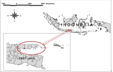
The study area of this research was the sea water of Madura Island, East Java Province, Indonesia; the south side is the Madura Strait and the north side is the Java Sea. It is located between 07°08' 30"S - 07°44' 27"S Latitude and 112°39' 23"E - 114°05' 24"E Longitude (Figure. 1).
2.2. Data Collection
[image:2.612.114.506.455.706.2]Data were collected from Madura Strait and the north side of Madura Island, or the Java Sea. It was collected twice: on November 23, 2015 (the researchers took the sea water of north area) and June 2, 2016 (the researchers took the sea water of south area along with the date of Landsat 8 passing by). The data required in this research were salinity, sulfate concentration, and reflectance remote sensing (Rrs) at sea surface. All data were taken at first hand for modeling algorithms and the image data is used as validation to test the implementation of the algorithm. Sea surface salinity and Band 5
5743 (NIR) Rrs of Landsat 8 OLI were the independent or predictor variable, while the sulfate concentration was the dependent variable or estimator.
2.3. Insitu Data Processing
The data of the sea surface salinity was taken using a refractometer. Collecting sulfate insitu data was done by taking seawater samples to be analyzed its sulfate concentration in the Laboratory of Environmental Engineering Department of ITS (Sepuluh November Institute of Technology) using turbidimetric method by means of UV-VIS spectrophotometer. While the data of surface Reflectance Remote Sensing (Rrs) was taken using TriOS Ramses spectroradiometer. Meantime, there were three types of data recorded by spectroradiometer TriOS Ramses; water upward radiance (Lu), downward radiance atmosphere (Ls)
and downward irradiance atmosphere (Ed) (Figure. 2) of which those values will be used later to calculate the Rrs value using formulas (1) and (2) since the Rrs cannot be directly taken on the field [8], [30], [31].
𝑅 𝜆 (1)
𝐿 𝜆 𝐿 𝜆 𝜌 𝐿 𝜆 (2)
where Lw (water leaving radiance /Wm-2sr-1) is the
radiance value obtained from the water column and the radiation reflected directly by the thin layer of the sea surface [32], Lu is upwelling radiance (Wm -2sr-1), Ls is downward radiance atmosphere (Wm -2sr-1), ρs is part of the reflectance which is on the
surface of the waters derived from the reflection of the sun. ρs can be calculated using the Fresnel formula [33][8], or be calculated using the constant value of the research results [34], or constant value 0.02 as in Nababan research [32].
In recording the data, the spectroradiometer TriOS Ramses used a hyper spectralsensor with 320nm-950nm wavelength range and 3.3nm interval; so then it was done some adjustment based on the characteristic of Landsat 8 which has 11 bands. Landsat 8 has a 400nm-13000nm wavelength range which is divided into 11 bands.
0 200 400 600 800 1000 1200 1400 1600
0.000 500.000 1000.000 1500.000
Intensity
m
W
/(m
^2
nm
)
Wavelength (nm)
upward radiance
0.000 200.000 400.000 600.000 800.000 1000.000
Intensity
m
W/(m^2
nm
)
Wavelength (nm)
downward radiance
0.00 5.00 10.00 15.00 20.00 25.00 30.00 35.00
0.000 500.000 1000.000 1500.000
In
ten
sity m
W
/(m
^2
n
m
)
Wavelength (nm)
[image:3.612.97.513.394.684.2]downward irradiance
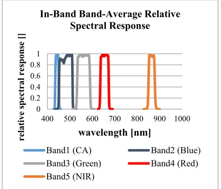
5744 In reducing Ramses data into Landsat 8 OLI characteristics, the researchers used the Relative Spectral Response (RSR) Landsat 8 value in calculating the mean of each band (Figure. 3) by using formula (3).
𝑅𝑆𝑅 ∆ ∑ :: .. ∆𝑅𝑆𝑅 (3)
where RSR is Relative Spectral Response and λ
is wavelength.
2.4. Satellite Data Processing
The Landsat 8 OLI images which were used as data tes of the algorithm model application were
available for free download on page
https://earthexplorer.usgs.gov/ or on
http://glovis.usgs.gov/ on path 118 and row 65. Landsat 8 OLI image taken out within the directory
of Landsat Collection 1 Level-2 (On-Demand) was
Landsat 8 OLI/TIRS C1 Level-2. Furthermore, to get
the value of sea surface Rrs for each pixel of Landsat 8 OLI image, the first calculation was the division of the pixel value by 10000 to obtain the reflectance value. The result was then divided by a constant value of pi (π) to find the sea surface Rrs.
2.5. Data Mining
Data mining can be defined as a process aimed at finding a pattern of amounts large data since data is useless without analysis [24]. Data mining can be interpreted as a process to find interesting patterns and descriptive models that can be understood and predictive of large-scale data [35] or the process of discovering useful patterns and trends in large [36].
data sets The data set can be nominally or
[image:4.612.318.522.172.211.2]numerically. Through this analysis allows one to gain knowledge and insight based on patterns obtained [35] as shown in Figure 4.
Figure 4: Process Diagram of Data Mining
In analyzing data mining requires a method then known as data mining algorithm [36]. Through the application of the algorithm will then obtain knowledge in patterns as useful information and can be used in decision making. Some of the most commonly used methods of data mining are description, estimation, prediction, classification, clustering, and association [36]. In this study used estimation method to estimate sulfate concentration at sea surface.
Estimation is part of the predictive analysis in data mining used to extract information from large data sets to make predictions and estimates about future outcomes [36]. The estimation algorithm that many develop using regression both linear and non linear [24], [35], [36]. In this study will also be used linear regression, non linear regression and multiple regression. In estimation, approximating the value of dependent (estimator) variable using a set of numeric and/or categorical independent (predictor) variables [36]. After the model, as the algorithm, is built subsequently used to estimate the new data of observations in the form of the value of the predictor variable then the value of the target of estimator variables will be obtained.
2.6. Regression Model
Regression is a statistical analysis technique to see functional relationship between two or more variables [37], [38]. In other literature, a variable can be predicted or estimated by other variables [39] by using regression calculation with The least-squares method. In regression equation there are independent variables known as predictor variable of which equation model written as X. While the dependent variable is the predicted or estimated response variable which is known as Y [38]. The predictor variable in regression can be more than one which is later known as multiple regression [40]. In certain literature, there are two models of regression: regression model for sample and population [41]. The equation forms of simple
0 0.2 0.4 0.6 0.8 1
400 500 600 700 800 900 1000
relative
sp
ectral
res
po
ns
e []
wavelength [nm] In-Band Band-Average Relative
Spectral Response
Band1 (CA) Band2 (Blue) Band3 (Green) Band4 (Red) Band5 (NIR)
Figure 3:Relative Spectral Response of Landsat 8 OLI
[image:4.612.85.301.242.427.2]
5745 linear regression are like formula (4) for population and formula (5) for sample. While multiple linear regression with more than one predictor variables are like formula (6) for population and formula (7) for sample [38].
𝑌 𝛽 𝛽 𝑋 𝜀 (4)
𝑌 𝑎 𝑏𝑋 (5)
𝑌 𝛽 𝛽 𝑋 𝛽 𝑋 … … 𝛽 𝑋 𝜀 (6)
𝑌 𝑎 𝑏 𝑋 𝑏 𝑋 … 𝑏 𝑋 (7)
Where Y is the estimated value (predictor variable), a/β0 is a constant value or intercept of the
regression coefficient of Y if the predictor variable is zero, b/β1 is a constant value or slope of regression
coefficient, and X / X1 is a predictor variable. While b2 / β2 is a constant value or slope of the second multiple regression coefficient up to n (bn / βn), and X2 is the predictor variable of the second multiple regressions up to n (Xn). In the use of regression algorithm model in estimating the value of an element to be compared with the actual value of the measurement results, an error value ε is involved as what stated in formula (4) and Formula (6).
Beside the linier regression, there is a nonlinear regression in which the predictor variable is a factor, fractional or exponent. Some nonlinear regression equations are logarithmic formula (8), exponential formula (9), polynomial formula (10), and power formula (11).
𝑌 𝑎 ln 𝑥 𝑏 (8)
𝑌 𝑎 𝐸𝑋𝑃 (9)
𝑌 𝑎 𝑏𝑥 𝑏 𝑥 (10)
𝑌 𝑎 𝑥 (11)
Where Y is the dependent variable to be estimated,
a is a constant value or intercept of the regression coefficient, X is an independent or predictor variable, b is a constant value or slope of the regression coefficient and b1 is the value of a
constant or slope of the regression coefficient of order 2 polynomial regression and could be up to order 6.
To select the best algorithm model which delivers consistent estimation between the result of the applied model and the result of insitu data collection, the researchers applied coefficient determination value (R2) like formula (12)[13], and
the amount of diversity or variability in Y variable is provided by a model or level of relationship between the dependent and independent variables. The range of values which was used was from 0 to 1. The algorithm model is considered good or has a very strong relationship between the dependent and independent variables if the determination coefficient closed to 1 and it is multiplied by 100% [42][43].
𝑅 ∑ ∑∑ ∑ ∑∑ ∑ (12)
Where R2 is determination coefficient, n is total
samples, X is an independent variable (predictor), and Y is a dependent variable (response). Apart of R2, the performance of the algorithm model can also
be seen from the accuracy of the data obtained from the calculation using the algorithm model (estimation) which later is compared to the insitu data (measurement results directly on the field or laboratory) in form of residue or error. The method used was Root Mean Square Error (RMSE) formula (13) and Normalized Mean Absolute Error (NMAE) index formula (14)[44],[45],[27]. RMSE was used to see the residue average of model performance, whereas NMAE was used to see the average of absolute error of model performance in percentage. In estimation algorithm model, the most important thing to consider is the RMSE or NMAE value rather than R2 since the researchers concerned at the
residue or error of the comparison between the estimation and the measurement data on the field.
𝑅𝑀𝑆𝐸 ∑ (13)
𝑁𝑀𝐴𝐸 100% ∑ 100 (14)
Where RMSE is Root Mean Square Error, N is total samples, Xesti is data value from the model result,
Xmeas is insitu data value from the measurement
results on the field or in laboratory, and NMAE is Normalized Mean Absolute Error.
5746
2. ALGORITHM DEVELOPMENT
2.1. Developing the Algorithm
The algorithm in this study is an expanded model of the previous algorithm which used a non-linear regression such as logarithmic [18]. In this study, the algorithm was constructed using both linear (Formula 5) and non-linear regression with various models (Formula 8, 9, 10 and 11), including the multiple regression with two independent variables (Formula 7).
The independent variable (predictor) used was Band 5 (NIR) insitu Rrs of Landsat 8 OLI and the dependent variable was the insitu sea surface sulfate. For the multiple regressions, the second dependent variable was the insitu salinity, as listed in Table 1.
Table 1: Sulfate, Salinity, and Band 5 (NIR) Rrs of L8 Insitu Data for Training
No Insitu Sulfate (mg/L)
Insitu Salinity
(psu)
Band 5 (NIR) Rrs of L8
Insitu nW/(m^2 nm)
1 2089.14 31.18 0.000724871 2 2433.00 31.15 0.001388778 3 1984.50 30.95 0.000596093 4 2285.54 30.78 0.000852525 5 2167.82 30.82 0.000470973 6 1747.79 30.89 0.000162041 7 1890.14 30.99 0.000250217 8 1910.80 30.91 5.19759E-05 9 2046.43 31.01 0.000295619 10 2256.04 31.18 0.000118129 11 2360.79 31.00 0.000437175 12 1837.07 31.18 0.000305518 13 2083.00 31.27 0.000380465 14 2058.72 31.25 0.000936818 15 2366.92 31.30 0.000639645 16 1984.50 31.27 0.000454784 17 2366.92 31.23 0.000420605 18 2.045.18 31.26 0.001150861 19 1.920.85 31.28 0.000635676
Then, plotting will be done between the band 5 (NIR) insitu Rrs of Landsat 8 OLI with insitu sulfate to develop the algorithm with the insitu sulfate data by a scatter graph to see trendline of various regression models both linear and non-linear (Formula 8, 9, 10 and 11) as shown in Figure 5. Where Figure 5a is scatter graph for linear trendline, Figure 5b is scatter graph for logarithmic trendline, Figure 5c is scatter graph for power trendline, Figure 5d is scatter graph for polynomial
trendline and Figure 5e is scatter graph for polynomial trendline.
Figure 4a: Scatter Graph for Linear Trendline
Figure 4b: Scatter graph for logarithmic trendline
Figure 4c. Scatter graph for power trendline
Figure 4d: Scatter Graph for Polynomial Trendline
y = 240956x + 1966.3 R² = 0.1784
1,500.00 2,500.00 3,500.00 4,500.00
0 0.001 0.002 0.003
MEASURED
S
ULFATE
(MG/
L)
MEASURED RRS (NIR) BAND 5 (SR -1)
S C A T T E R W I T H L I N E A R T R E N D L I N E
y = 101ln(x) + 2881.4 R² = 0.1657
1,500.00 2,500.00 3,500.00 4,500.00
0 0.001 0.002 0.003
MEASURED
S
ULFATE
(MG/L)
MEASURED RRS (NIR) BAND 5 NW/(M^2 NM) S C A T T E R W I T H L O G A R I T H M I C
T R E N D L I N E
y = -3E+07x2+ 281572x + 1956.5 R² = 0.1788
1,500.00 2,500.00 3,500.00 4,500.00
0 0.001 0.002 0.003
MEASURED
S
ULFATE
(MG/
L)
MEASURED RRS (NIR) BAND 5 NW/(M^2 NM)) S C A T T E R W I T H P O L Y N O M I A L
T R E N D L I N E y = 3055.5x0.049
R² = 0.172
1,500.00 2,500.00 3,500.00 4,500.00
0 0.001 0.002 0.003
MEASURED
S
ULFATE
(MG/L)
MEASURED RRS (NIR) BAND 5 NW/(M^2 NM) S C A T T E R W I T H P O W E R
[image:7.612.88.300.78.239.2]
5747 Figure 4e: Scatter Graph for Polynomial Trendline
While the multiple regression with two predictor variables (X1, X2), band 5 (NIR) insitu Rrs
of Landsat 8 OLI as X1and sea surface salinity as
X2, was calculated using formula (15):
∑ 𝑌 𝑎𝑁 𝛽 ∑ 𝑋 𝛽 ∑ 𝑋 … … … … ∑ 𝑋 𝑌 𝑎 ∑ 𝑋 𝛽 ∑ 𝑋 𝛽 ∑ 𝑋 𝑋 ∑ 𝑋 𝑌 𝑎 ∑ 𝑋 𝛽 ∑ 𝑋 𝑋 𝛽 ∑ 𝑋
(15)
Where Y is dependent variable (response), X1and
X2 are first and second independent variables
(predictor). The results of modeling with multiple regression using formula (15) was the value of coefficient a (intercept) = 1550.54, X1/Rrs =
13.40andX2/SSS) = 239214.45 with significant value > 0.05, i.e. 0.20746954738219. While the determination coefficient (R2) using formula (12)
[image:7.612.314.520.539.723.2]was 0.1785. From several regression equations obtained from the results of model compilation for sulfate estimation algorithm at sea surface, the researchers obtained five algorithms as in (Table 2).
Table 2: Models of Estimation Algorithm for Sea Surface Sulfate
No Regression Model R2
1 Linear y = 240956x + 1966.3 0.1784
2 Exponential y = 1960.8exp115.82x 0.1815
3 Logarithmic y = 101ln(x) + 2881.4 0.1657
4 Polynomial y = -3E+07x2 + 281572x + 1956.5
0.1788
5 Power y = 3055.5x0.049 0.1720
6 Multiple
Regression 1550.54+13.40(SSS)+ 239214.45(Rrs) 0.1785
Where y is sea surface sulfate (dependent variable) and x is band 5 (NIR) Rrs of Landsat 8 OLI (independent variable). Rrs is reflectance remote
sensing of band 5 (NIR) from Landsat 8 OLI at sea surface and SSS is sea surface salinity.
From the five algorithms, it showed that the value of R2 was low. It meant that the band 5 (NIR)
Rrs of Landsat 8 OLI had a low functional relationship with seawater sulfate. Then, the researchers considered the value of RMSE and NMAE of the five algorithms when they were validated and tested with other data, and the selection of this estimation algorithm depended on the RMSE and NMAE values.
2.1. Model Validation and Testing
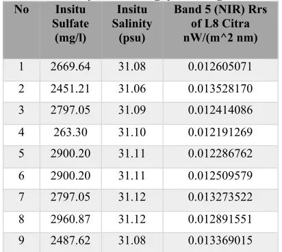
The six models were then validated and tested using the RRS of Landsat 8 OLI data which were taken on different dates to see the performance of the model as the estimation algorithm of sulfates at sea surface (Table 3). Landsat 8 OLI image was downloaded on https://earthexplorer.usgs.gov/ on November 3, 2015. In the same date, the researchers took insitu sulfate data as the comparator to validate the data obtained from the estimation of the algorithm model. Next, the 10 data in Table 3 were then divided into two; five data for validation and five data for testing.
The results of validation and testing of the data using formula (13) and formula (14) as in Table 4. There, the data showed that the power regression model had better performance than other models. The evidence were the smaller NMAE and RMSE values compared to other models, 9.36% and 299.66 respectively for validation; 9.53% and 320.84 for the test. Thus, by considering the related results of estimation, the algorithm model selected for this current research was the power regression with coefficient value a (intercept) = 3055.5 and coefficient value b (slope) = 0.049.
Table 3: Insitu Sulfate, Insitu Salinity, and Band 5 (NIR) Rrs of L8 OLI Image for Testing
No Insitu Sulfate
(mg/l)
Insitu Salinity
(psu)
Band 5 (NIR) Rrs of L8 Citra nW/(m^2 nm)
1 2669.64 31.08 0.012605071
2 2451.21 31.06 0.013528170 3 2797.05 31.09 0.012414086 4 263.30 31.10 0.012191269 5 2900.20 31.11 0.012286762 6 2900.20 31.11 0.012509579 7 2797.05 31.12 0.013273522
8 2960.87 31.12 0.012891551 9 2487.62 31.08 0.013369015 y = 1960.8e115.82x
R² = 0.1815
1,500.00 2,500.00 3,500.00 4,500.00
0 0.001 0.002 0.003
MEASURED
S
ULFATE
(MG/
L)
MEASURED RRS (NIR) BAND 5 NW/(M^2 NM) S C A T T E R W I T H E X P O N E N T I A L
[image:7.612.84.301.545.687.2]
5748
10 2706.05 31.07 0.014069297
Table 4: NMAE and RMSE values of Each Regression Model
3. ALGORITHM IMPLEMENTATION
The developed algorithm was then
implemented into the data of Landsat 8 OLI as distribution media of sulfate mapping at sea surface. Algorithm application and image processing were done by using Beam Visat software started from the change of the digital number on the image pixel into Rrs sea surface.
The first thing to do was inserting the Band 5 (NIR) Landsat 8 OLI image into the Beam Visat editor. Next, the image was processed by changing a DN of image pixel into surface reflectance values by dividing DN by 10000 and phi constant value that was put into Band Maths Expression Editor on
Beam Visat software as shown in Figure. 5. The
result of this process was an image with a pixel value of sea surface Rrs on Band 5 (NIR) of Landsat 8 OLI (Figure 6)
Figure 5: Converting DN of Image Pixel Into Sea Surface Rrs
Figure 6: The Image with Rrs Pixel Value
The second was inserting the estimation algorithm (the formula in Table 2, number 5) into Band Maths Expression Editor on Beam Visat
software (Figure. 7). The result showed that each image pixel was converted into sulfate value.
Figure. 7. Entering the Sulfate Estimation Algorithm in Band Maths Expression Editor of Beam Visat
When the algorithm was implemented, the model converted all pixels into sulfate values for both land and water object. So, in this case, the researchers separated the mainland pixel and the water pixel using formula (16) that was shown in
Figure 8. Since the researchers only separated sulfate values, the word ‘unsur’ was changed into sulfate (Figure 9). Therefore, the result was the image of sulfate distribution at sea surface in Madura strait (Figure 10).
𝑁𝐷𝑊𝐼 0? 𝑢𝑛𝑠𝑢𝑟 ∶ 0 (16)
𝑁𝐷𝑊𝐼 (17)
Where NDWI (Normalized Difference Water Index) was the algorithm to separate water and land pixels on the image by creating a water value index. The result was the NDWI values and classified into
No Regression Validation Testing
NMAE (%)
RMSE
(sr-1) NMAE (%) RMSE (sr-1) 1 Linear 85.55 2328.86 88.00 2393.29
2 Exponential 217.79 5932.02 228.10 6223.39
3 Logarithmic 10.34 323.11 10.15 343.08
4 Polynomial 76.61 2092.41 81.39 2242.16
5 Power 9.36 299.66 9.53 320.84
6 Multiple
[image:9.612.314.520.143.288.2]
5749 2: when it was greater than 0, it was defined as water zone. In contrast, if the NDWI was smaller or equal to 0, then the zone was defined as mainland. RRS value used to calculate NDWI was Reflectance Remote Sensing of band 3 and 5 of Landsat 8 OLI imagery.
[image:9.612.92.299.175.315.2]Figure 8: NDWI Algorithm Application
[image:9.612.91.299.350.515.2]Figure 9: The Classification of Sulfate Values in Aquatic Pixels with NDWI Value
Figure 10: The distribution of Sulfate Concentration at Sea Surface in Madura Strait Waters
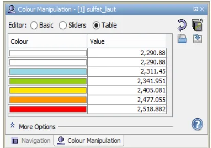
The picture on Figure 10 shows the color gradation which represents the distribution of sulfate concentration at the sea surface of Madura Strait. There were 5 color gradations which indicated the degree of sulfate concentration at the sea surface of Madura Strait starting from white
which represented the lowest sulfate concentration, i.e. 2290.88 and red which represented the highest sulfate concentration, i.e. 2518.882 (Figure 11).
Figure 11: The color class of sulfate distribution at sea surface in Madura Strait
Highest sulfate concentration zone was near the beach with high public activities like Kamal harbor, Bangkalan regency. In addition, the general overview of the statistic, minimum pixel value was 0 and the maximum value was 8248.489 (Figure 12).
The data of sulfate concentration obtained from the estimation algorithm which was compared to insitu sulfate by utilizing Landsat 8 OLI image data showed NMAE 9.53% and RMSE 320.84 of which showed little error and low residue level.
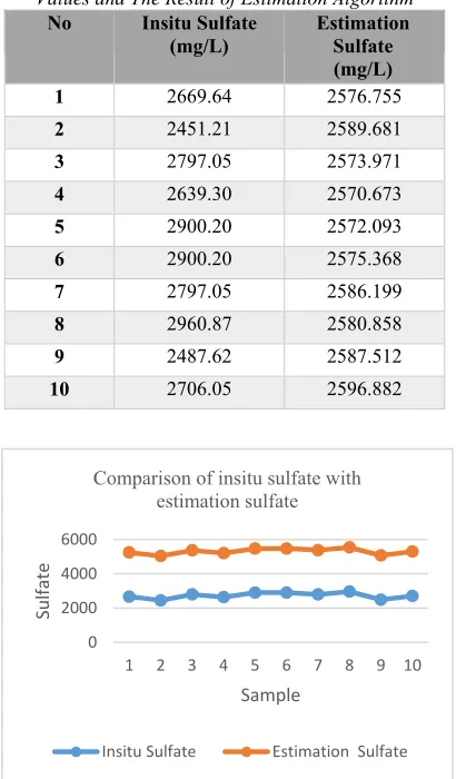
[image:9.612.89.299.511.630.2]Table 5 and Figure 13 showed differences of the sulfate concentration values obtained from the estimation algorithm and the insitu data that were extracted from the pixel of Landsat 8 OLI image. Both of them referred to the same coordinate point of which the image data and seawater samples were taken.
[image:9.612.319.522.545.691.2][image:10.612.92.297.110.460.2]
5750 Table 5: Comparison of Insitu Sulfate Concentration
Values and The Result of Estimation Algorithm
Figure 13: Graphic comparison of insitu sulfate values and the result of estimation algorithm
4. DISCUSSION
Development of a model, as an estimation algorithm sulfate in sea surface, is intended to improve the performance of model itself. The indicators used in addition to the reliability and usefulness of the model to estimate are the accuracy of data which result of model application compared with the field data. Among several methods that can be used to evaluate the accuracy of model applications are NMAE and RMSE. Both models, previous research results [18] and current research, will be applied to the same data ie Rrs values in band 5 (NIR) of Landsat 8 OLI image. Another similarity is the region and time of field data retrieval (Table 3).
In the previous model [18], each variable data value (X and Y) convert to log value. Then enter into a model which is a logarithmic regression equation and the result is still a log value. To
convert into sulfate value, the result value of the model is made a power of 10 since the log used is base-10. By using the Formula (13) and Formula (14) obtained values of NMAE and RMSE as in
Table 6.
Table 6: Values of NMAE and RMSE of Previous dan Current Research
Research Adjusted Model NMAE %
RMSE sr-1
Previous 103.8033– 0.411ln(log(RrsNIR)) 75.8 8688
Current 3055.5RrsNIR0,049 9.5 320
Table 6 shows the value of NMAE and RMSE on the previous model is very high, respectively 75.8% and 8688 sr-1. While for the
current research the values of NMAE and RMSE only 9.5% and 343 sr-1. This occurs because
previous models [18] were built using less data than the current research. Wherein the use of data mining to get patterns more accurately using a lot of data since of variations in value will determine the type of pattern and the information will be obtained.
This research was done in the regional waters of the Madura strait-Indonesia with a tropical climate and then the data is collect in the dry season. With the region's characteristics the influence of the atmosphere and the latitude position on the equator line will affect the satellite recording of the reflectance spectra (Rrs) of the sea surface and the sulfate concentration in sea water. So that territorial use of this algorithm can be evaluated to produce a more optimal estimation value when will be used in other regions with very different characteristics.
The use of Rrs from Band 5 (NIR) of Landsat 8 OLI imagery is based on previous research [52] showed that among the band 1 (CA), band 2 (blue), the band 3 (green), band 4 (red), and band 5 (NIR), as measured by tool Spectroradiometer TriOS Ramses, which is sensitive (spectral signature) to sulfate in sea surface is a band 5 (NIR). Then there are other studies also using band 5 (NIR) for modeling near-infrared reflectance spectra of clay and sulfate mixtures and implications for Mars [53].
5. CONCLUSIONS
The authors have evaluated the performances of the previous research model as estimation algorithm to estimate a sulfate concentration at the sea surface. By using NMAE and RMSE values have been obtained that the model of current research is smaller than previous research, No Insitu Sulfate
(mg/L) Estimation Sulfate (mg/L) 1 2669.64 2576.755
2 2451.21 2589.681
3 2797.05 2573.971
4 2639.30 2570.673
5 2900.20 2572.093
6 2900.20 2575.368
7 2797.05 2586.199
8 2960.87 2580.858
9 2487.62 2587.512
10 2706.05 2596.882
0 2000 4000 6000
1 2 3 4 5 6 7 8 9 10
Sulfate
Sample
Comparison of insitu sulfate with estimation sulfate
5751 respectively 9.5% and 320.8 sr-1. While previous
research has NMAE and RMSE values respectively 75.8% and 8688 sr-1.
The developed estimation algorithm of the sea surface sulfate concentration using both linear and non-linear regression model obtained non-linear model: a power regression with higher degree of precision and smaller value of average error and residue. The algorithm can be applied to estimate sulfate concentration at sea surface with the value obtained for coefficient a (intercept) 3055.5 and coefficient b (slope) 0.049 and one predictor variable (X) that was band 5 (NIR) Rrs of Landsat 8 OLI. In addition, the correlation functionality between sulfate and band 5 (NIR) Rrs of Landsat 8 OLI imagery was low with R2 value only 0.1720 or
1.72% Rrs as the estimation factor of sulfate concentration at sea surface.
ACKNOWLEDGMENT
The researchers thank to the Indonesian National Institute of Aeronautics and Space for the support of data collection.
REFERENCES
[1] R. Chang, CHEMISTRY 10th EDITION, 10th ed. New York: The McGraw-Hill Companies, 2010.
[2] R. Chang and J. Overby, General Chemistry
The Essential Concepts (Sixth Edition), 6th
ed. New York: The McGraw-Hill Companies, 2011.
[3] P. Aji and R. Purwanto, Pengendalian Mutu
Beton Sesuai SNI, ACI dan ASTM. Surabaya:
ITS Press, 2010.
[4] M. Effendy, Model Algoritma Pendugaan Konsentrasi Klorofil-a Berdasarkan Data Citra Satelit Landsat ETM+ untuk Pemetaan
Lokasi Fishing Ground di Madura.
Bangkalan: Fakultas Pertanian, Universitas Trunojoyo Madura, 2009.
[5] F. Wang and Y. J. Xu, “Development and application of a remote sensing-based salinity prediction model for a large estuarine lake in the US Gulf of Mexico coast,” pp. 184–194, 2008.
[6] S. Scale, “SATELLITE REMOTE
SENSING : SALINITY
MEASUREMENTS,” pp. 127–132, 2009. [7] Y. H. Ahn., P. Shanmugam, J. E. Moon, and
J. H. Ryu, “Satellite remote sensing of a low-salinity water plume in the East China Sea,”
Ann. Geophys., vol. 26, no. 7, pp. 2019–2035,
2008.
[8] S. Budhiman, M. Suhyb, Z. Vekerdy, and W.
Verhoef, “Deriving optical properties of Mahakam Delta coastal waters , Indonesia using in situ measurements and ocean color model inversion,” ISPRS J. Photogramm.
Remote Sens., vol. 68, pp. 157–169, 2012.
[9] T. Lillesand, R. W. Kiefer, and J. Chipman,
Remote Sensing and Image Interpretation, 7th
Edition, Fifth Edit. New York: John Wiley &
Sons, 2015.
[10] J. George, Fundamentals of Remote Sensing, Second Edi. Hyderabad: Universities Press (India), 2005.
[11] Y. Liu, M. A. Islam, and J. Gao, “Quantification of shallow water quality parameters by means of remote sensing,”
Prog. Phys. Geogr., vol. 27, no. 1, pp. 24–43,
2003.
[12] M. A. Syariz et al., “RETRIEVAL OF SEA
SURFACE TEMPERATURE OVER
POTERAN ISLAND WATERS OF
INDONESIA WITH LANDSAT 8 TIRS
IMAGE : A PRELIMINARY
ALGORITHM,” 2015.
[13] P. J. Werdell et al., “Retrieving marine inherent optical properties from satellites using temperature and salinity- dependent backscattering by seawater,” vol. 21, no. 26, pp. 32611–32622, 2013.
[14] A. Matsuoka, M. Babin, and E. C. Devred, “Remote Sensing of Environment A new algorithm for discriminating water sources from space : A case study for the southern Beaufort Sea using MODIS ocean color and SMOS salinity data,” Remote Sens. Environ., vol. 184, pp. 124–138, 2016.
[15] Y. Bai, D. Pan, W. Cai, X. He, D. Wang, and B. Tao, “Remote sensing of salinity from satellite-derived CDOM in the Changjiang River dominated East China Sea,” J. Geophys.
Res. Ocean., vol. 118, pp. 227–243, 2013.
[16] K. Shi, Y. Zhang, X. Liu, M. Wang, and B. Qin, “Remote Sensing of Environment Remote sensing of diffuse attenuation coef fi cient of photosynthetically active radiation in Lake Taihu using MERIS data,” Remote Sens.
Environ., vol. 140, pp. 365–377, 2014.
[17] L. M. Jaelani, F. Setiawan, and H. Wibowo, “Pemetaan Distribusi Spasial Konsentrasi Klorofil-a dengan Landsat 8 di Danau Towuti dan Danau Matano , Sulawesi Selatan,” Pros. Pertem. Ilm. Tahun Masy. Penginderaan Jauh
Indones., vol. XX, 2015.
5752 OLI,” in Konferensi Nasional Teknik Sipil dan
Infrastruktur, 2017, pp. 13–22.
[19] I. H. Witten and E. Frank, Data Mining Practical Machine Learning Tools and
Techniques, Second. Elsevier Inc., 2005.
[20] B. Trisakti, “STANDARISASI KOREKSI DATA SATELIT MULTI TEMPORAL DAN MULTI SENSOR ( LANDSAT TM / ETM + DAN SPOT-4 ).”
[21] B. M. Sukojo and Wahono, “Pemanfaatan Teknologi Penginderaan Jauh untuk Pemetaan Kandungan Bahan Organik Tanah,” Makara,
Teknol., vol. 6, no. 3, pp. 102–112, 2002.
[22] Z. Lee and K. L. Carder, “Diffuse Attenuation Coefficient of Downwelling Irradiance : An Evaluation of Remote Sensing Methods,” J.
Geophys. Res., vol. 110, no. 10, 2005.
[23] Z. Lee, S. Shang, L. Qi, J. Yan, and G. Lin, “Remote Sensing of Environment A semi-analytical scheme to estimate Secchi-disk depth from Landsat-8 measurements,” Remote
Sens. Environ., vol. 177, pp. 101–106, 2016.
[24] N. Ye, Data Mining (Theories, Algorithms,
and Examples). Taylor & Francis Group,
LLC, 2014.
[25] A. Simon and P. Shanmugam, “A model to predict spatial , spectral and vertical changes in the average cosine of the underwater light fi elds : Implications for remote sensing of shelf-sea waters,” Cont. Shelf Res., vol. 116, pp. 27–41, 2016.
[26] M. R. Khomarudin, P. Bidang, P. Data, and P. Jauh, “APLIASI PENGINDERAAN JAUH UNTUK MENDUGA UNSUR IKLIM DAN PRODUKTIVITAS TANAMAN HUTAN,” vol. 6, no. 2, pp. 50–61, 2004.
[27] T. Chai and R. R. Draxler, “Root mean square error ( RMSE ) or mean absolute error ( MAE )? – Arguments against avoiding RMSE in the literature,” Geosci. Model Dev., vol. 7, no. 3, pp. 1247–1250, 2014.
[28] C. J. Willmott and K. Matsuura, “Advantages of the Mean Absolute Error ( MAE ) Over the Root Mean Square Error ( RMSE ) in Assessing Average Model Performance,”
Clim. Res., vol. 30, no. 1, pp. 79–82, 2005.
[29] S. Xian-Zhong, A. Mehrooz, and O. David, “Reflectance Spectral Characterization And Mineralogy Of Acid Sulphate Soil In Subsurface Using Hyperspectral Data,” Int. J.
Sediment Res., vol. 29, 2014.
[30] S. Budhiman, “Perbandingan Karakteristik Spektral (Spectral Signature) Parameter Kualitas Perairan Pada Kanal Landsat ETM + dan Envisat Meris (Comparion of Water
Constituents Spectral Signature on Landsat
ETM+ and Envisat Meris Band,” J.
Pengideraan Jauh, vol. 9, no. 2, pp. 76–89,
2012.
[31] C. D. Mobley, “Estimation of Remote Sensing
Reflectance from Above-Surface
Measurements,” Appl. Opt., vol. 38, no. 36, pp. 7442–7455, 1999.
[32] B. Nababan, A. A. Wirapramana, and R. E. Arhatin, “Spectral of Remote Sensing Reflectance of Surface Waters,” J. Ilmu dan
Teknol. Kelaut. Trop., vol. 5, no. 1, pp. 69–84,
2013.
[33] E. Hecht, OPTICS fourth edition, 4th ed. Addison-Wesley, 2002.
[34] C. D. Mobley, “Estimation of the remote-sensing reflectance from above-surface measurements,” 1999.
[35] M. J. Zaki and W. M. Jr, Data Mining and Analysis Fundamental Concepts and
Algorithms. New York: Cambridge University
Press, 2014.
[36] D. T. Larose and C. D. Larose, Data Mining
and Predictive Analytics, Second. Canada:
John Wiley & Sons, Inc., 2015.
[37] R. E. Walpole, Pengantar Statistik. Edisi ke-3
in Bambang Sumantri (Ed). Jakarta: PT
Gramedia Pustaka Utama, 1995.
[38] J. Supranto, Statistik : Teori dan Aplikasi. Jakarta: Erlangga, 2001.
[39] Kismianti, “Handout Analisis Regresi,” Yogyakarta, 2010.
[40] D. N. Gujarati, Basic Econometrics, Fourth
Edition, 4th ed. Colombus: The McGraw-Hill
Companies, 2004.
[41] Y. Ahmad, “Materi Kuliah Metode Statistika (Regresi dan Korelasi),” Cianjur, 2007. [42] J. Chen, T. Cui, J. Ishizaka, and C. Lin,
“Remote Sensing of Environment
Corrigendum to ‘ A neural network model for remote sensing of diffuse attenuation coef fi cient in global oceanic and coastal waters : Exemplifying the applicability of the model to the coastal regions in Eastern China Seas ’ [ Remote Sensing of Environment , 148 168 – 177 ],” Remote Sens. Environ., vol. 153, pp. 99–103, 2014.
[43] J. Zhao, M. Temimi, and H. Ghedira, “Remotely sensed sea surface salinity in the hyper-saline Arabian Gulf : application to Landsat 8 OLI data,” Estuar. Coast. Shelf Sci., 2017.
5753 2, pp. 133–151, 2001.
[45] J. P.H.M. and H. P.S.C., “Calibration of Process-Oriented Models,” Ecol. Modell., vol. 83, no. 1–2, pp. 55–66, 1995.
[46] S. Son and M. Wang, “Remote Sensing of Environment Diffuse attenuation coef fi cient of the photosynthetically available radiation K d ( PAR ) for global open ocean and coastal waters,” Remote Sens. Environ., vol. 159, pp. 250–258, 2015.
[47] K. A. Semmens et al., “Remote Sensing of
Environment Monitoring daily
evapotranspiration over two California vineyards using Landsat 8 in a multi-sensor data fusion approach,” 2015.
[48] X. Yu, M. Suhyb, F. Shen, and W. Verhoef, “Remote Sensing of Environment Retrieval of the diffuse attenuation coef fi cient from GOCI images using the 2SeaColor model : A case study in the Yangtze Estuary,” Remote
Sens. Environ., vol. 175, pp. 109–119, 2016.
[49] Z. Zheng, J. Ren, Y. Li, C. Huang, and G. Liu, “Science of the Total Environment Remote sensing of diffuse attenuation coef fi cient patterns from Landsat 8 OLI imagery of turbid inland waters : A case study of Dongting Lake,” Sci. Total Environ., vol. 573, pp. 39– 54, 2016.
[50] S. Mckeen et al., “Assessment of an ensemble of seven real-time ozone forecasts over eastern North America during the summer of 2004,” J. Geophys. Res., vol. 110, pp. 1–16, 2005.
[51] Y. B. Son et al., “Tracing offshore low-salinity plumes in the Northeastern Gulf of Mexico during the summer season by use of multispectral remote-sensing data,” J.
Oceanogr., vol. 68, no. 5, pp. 743–760, 2012.
[52] Muhsi, “ANALISA KARAKTERISTIK SPEKTRAL ( SPECTRAL SIGNATURE ) UNTUK SULFAT DI PERMUKAAN AIR LAUT PADA BAND LANDSAT 8 OLI,” in
Seminar Nasional Humaniora dan Aplikasi
Teknologi Informasi, 2016, vol. 2016, no.
Sehati, pp. 16–17.
[53] K. M. Stack and R. E. Milliken, “Modeling near-infrared reflectance spectra of clay and sulfate mixtures and implications for Mars,”
Icarus, vol. 250, pp. 332–356, 2015.