Improved Techniques in Ultrasonic Molecular Imaging for Evaluating Response to Cancer Therapy
Jason E. Streeter
A dissertation submitted to the faculty of the University of North Carolina at Chapel Hill in partial fulfillment of the requirements for the degree of Doctor of Philosophy in the Department of Biomedical Engineering.
Chapel Hill 2013
Approved by:
c
2013
Abstract
JASON E. STREETER: Improved Techniques in Ultrasonic Molecular Imaging for Evaluating Response to Cancer Therapy.
(Under the direction of Paul A. Dayton, Ph.D.)
Molecular imaging is a broad term for describing a technique designed to evaluate molecular activity in biological systems. Recently, ultrasound has gained interest in molecular imaging due to the practical advantages over traditional imaging modalities: it is inexpensive, safe and portable.
The principle behind ultrasonic molecular imaging (USMI) is the selective target-ing of acoustically active intravascular microbubbles to biomarkers expressed on the endothelium. Once accumulated at the target site, the microbubbles enhance the acous-tic backscatter from pathologic tissue that might otherwise be difficult to distinguish from normal tissues. Since USMI has the potential to provide information prior to the appearance of phenotypic changes, it is proposed that this method can facilitate early assessment of disease progression. Pre-clinical imaging studies have demonstrated the efficacy of USMI for applications including, but not limited to, assessment of tumor angiogenesis, evaluation of cardiovascular disease, and imaging dysfunctional endothe-lium, thrombus and inflammation.
Although significant advances in USMI have been made, there remain challenges that need to be addressed as this technique advances toward clinical relevance. The ultimate goal of USMI is to determine the degree to which biomarkers are expressed by the target tissue. Therefore, it is essential that targeted microbubbles adhere in quantities that produce backscattered intensities in greater magnitude than the signal
from non-specific targeting. Given this requirement, research has primarily focused on improving the sensitivity to bound microbubbles, improving the ability to quantify biomarker expression, increasing the quantity of targeted microbubbles retained at the site of pathology, and improving microbubble architecture to minimize the non-specific retention of microbubbles and immunogenic response.
This dissertation supports the following hypotheses for in vivo USMI experiments:
1. Producing size-selected microbubbles increases detection sensitivity.
2. Implementing a 3-D ultrasound platform improves our ability to quantify biomarker expression.
3. Using acoustic radiation force enhances microbubble targeting.
4. Creating buried-ligand microbubbles reduces immunogenic response and non-specific targeting.
This is dedicated to my family, for their patience,
for their encouragement, for their support, and for their love.
Acknowledgments
Table of Contents
Table of Contents . . . vii
List of Figures . . . xiv
List of Tables . . . xvii
List of Abbreviations . . . xviii
1 Hypotheses and Scope . . . 1
1.1 Hypotheses . . . 1
1.2 Scope . . . 1
2 Overview of Cancer . . . 4
2.1 Cancer Overview . . . 4
2.2 Cancer Statistics . . . 4
2.3 Early Detection of Cancer . . . 7
2.4 Personalized Cancer Therapy . . . 7
2.5 Response to Cancer Therapy . . . 8
3 Molecular Imaging Overview . . . 10
3.1 Molecular Imaging . . . 10
3.1.1 Metabolic Imaging with PET . . . 11
3.1.2 Imaging angiogenesis with PET . . . 11
3.1.3 Imaging angiogenesis with SPECT . . . 12
3.1.4 Optical Imaging . . . 12
3.2 USMI Introduction . . . 13
3.2.1 Sensitivity Improvement . . . 15
3.2.2 Quantification Improvement . . . 16
3.2.3 Improvement in Quantity of Targeted MCAs . . . 17
3.2.4 Immunogenic Response Minimization . . . 18
3.3 Summary . . . 19
4 Microbubble Contrast Agents . . . 20
4.1 Microbubble Contrast Agents . . . 20
4.1.1 Microbubbles for Perfusion Imaging . . . 21
4.1.2 Microbubbles for Molecular Imaging . . . 22
4.2 Microbubble Safety . . . 23
4.3 Experimental Methods for MCA Fabrication . . . 24
4.3.1 Perfusion Agent Recipe . . . 24
4.3.2 Non-targeted Agent Recipe . . . 24
4.3.3 Targeted Agent Recipe . . . 24
4.3.4 Lipid Preparation Procedure . . . 25
4.3.5 Unsorted Microbubble Populations . . . 26
4.3.6 Sorted Microbubble Populations . . . 26
5 Imaging and Animal Preparation . . . 33
5.1 Imaging Contrast Agents . . . 33
5.1.1 Amplitude Modulation Imaging Overview . . . 34
5.1.2 Pulse Inversion Imaging Overview . . . 34
5.1.4 Harmonic and Sub-Harmonic Imaging Overview . . . 37
5.2 Experimental Methods - Imaging System . . . 38
5.2.1 System overview and capabilities . . . 38
5.2.2 Experimental Methods - CPS Imaging . . . 40
5.2.3 Experimental Methods - 3-D Imaging Apparatus . . . 40
5.2.4 Experimental Methods - ARF for MCA Translation . . . 40
5.3 Animal Preparation and MCA Administration . . . 41
5.3.1 Tissue Implantation . . . 41
5.3.2 Animal Preparation for Imaging . . . 42
5.3.3 Contrast Administration . . . 42
6 Experimental Diagnostic Methods . . . 44
6.1 Perfusion-Based Imaging and Methods . . . 44
6.1.1 Time-Intensity . . . 45
6.1.2 Destruction-Reperfusion . . . 48
6.2 Molecular Imaging and Methods . . . 51
7 Repeated Administration of Targeted Contrast Agents . . . 56
7.1 Introduction . . . 56
7.2 Materials and Methods . . . 58
7.2.1 Microbubble Contrast Agents . . . 58
7.2.2 Animals and Tumor Models . . . 58
7.2.3 Clinical Imaging System . . . 58
7.2.4 Molecular Imaging Protocol . . . 58
7.3 Results . . . 59
7.4 Discussion and Conclusion . . . 61
8 Improving Sensitivity in USMI . . . 62
8.1 Introduction . . . 62
8.2 Materials & Methods . . . 64
8.2.1 Microbubble Contrast Agents . . . 64
8.2.2 Animal Preparation and Contrast Administration . . . 65
8.2.3 Imaging System . . . 66
8.2.4 Perfusion Imaging . . . 66
8.2.5 Molecular Imaging . . . 67
8.3 Results . . . 67
8.3.1 Perfusion Imaging (Intensity & Persistence) . . . 67
8.3.2 Molecular Imaging . . . 70
8.4 Discussion and Conclusion . . . 71
9 3-D US MI of Angiogenesis . . . 78
9.1 Introduction . . . 78
9.2 Materials & Methods . . . 79
9.2.1 Microbubble Contrast Agents . . . 79
9.2.2 Animal Preparation and Contrast Administration . . . 79
9.2.3 3-D Imaging Apparatus . . . 79
9.2.4 Image Acquisition . . . 80
9.2.5 Multi-slice IHC Analysis . . . 80
9.3 Results . . . 83
9.3.1 Intra-tumor Analysis . . . 83
9.3.2 Inter-tumor Analysis . . . 85
9.3.3 Approximating Error in Analogous 2-D Study . . . 86
9.3.4 Multi-slice IHC Analysis . . . 87
10 Arf-Enhanced USMI . . . 93
10.1 Introduction . . . 93
10.1.1 Background . . . 93
10.1.2 ARF and Molecular Imaging . . . 94
10.2 Materials & Methods . . . 96
10.2.1 Microbubble Contrast Agents . . . 96
10.2.2 Imaging System . . . 96
10.2.3 Calibration . . . 97
10.2.4 Effect of ARF Pressure . . . 97
10.2.5 Estimating Optimal In Vivo Study Parameters . . . 101
10.2.6 In Vivo Experiments . . . 102
10.3 Results . . . 104
10.3.1 Effect of ARF Pressure . . . 104
10.3.2 Estimating Optimal In Vivo Study Parameters . . . 105
10.3.3 In Vivo Results . . . 106
10.4 Discussion and Conclusion . . . 111
10.4.1 In Vitro Predictions and In Vivo Results . . . 111
10.4.2 Comparing This In Vivo Study To Previous Work . . . 112
10.4.3 Limitations and Future Directions . . . 114
11 USMI with Buried-Ligand Microbubbles . . . 117
11.1 Introduction . . . 117
11.2 Materials and Methods . . . 119
11.2.1 Microbubble Contrast Agents . . . 119
11.2.2 Animals and Tumor Models . . . 119
11.2.3 Clinical Imaging System . . . 120
11.2.4 Imaging System . . . 120
11.2.5 Contrast Agent Persistence Protocol . . . 120
11.2.6 Molecular Imaging Protocol . . . 121
11.3 Results . . . 121
11.3.1 Contrast Agent Persistence In Vivo . . . 121
11.3.2 Molecular Imaging In Vivo . . . 122
11.4 Discussion and Conclusion . . . 124
12 Evaluating Techniques for Response to Therapy . . . 127
12.1 Introduction . . . 127
12.1.1 Aurora-A Kinase Inhibition . . . 127
12.1.2 Response to therapy . . . 128
12.1.3 Ultrasonic Molecular Imaging . . . 128
12.1.4 Dynamic Contrast-Enhanced Perfusion Imaging . . . 129
12.2 Materials and Methods . . . 130
12.2.1 Microbubble Contrast Agents . . . 130
12.2.2 Animal Preparation and Contrast Administration . . . 131
12.2.3 Therapy . . . 131
12.2.4 3-D Imaging Apparatus . . . 132
12.2.5 Ultrasonic Molecular Imaging . . . 132
12.2.6 Dynamic Contrast-Enhanced Perfusion Imaging . . . 133
12.2.7 Volume Measurements . . . 133
12.3 Results . . . 133
12.3.1 Ultrasonic Molecular Imaging . . . 133
12.3.2 Dynamic Contrast-Enhanced Perfusion Imaging . . . 135
12.3.3 Volume Measurements . . . 136
13 Discussion and Conclusion . . . 143
13.1 Introduction . . . 143
13.2 Discussion - Improved USMI Techniques . . . 145
13.2.1 Repeated Injections in an USMI Study . . . 145
13.2.2 Size-Selection for Sensitivity Improvement . . . 146
13.2.3 3-D for Improved Quantification . . . 148
13.2.4 ARF-Enhanced USMI for Improved Adherence . . . 149
13.2.5 BLA for Reduced Immunogenic Response . . . 151
13.3 Discussion - Response to Therapy . . . 152
13.4 Discussion - Clinical Translation . . . 155
13.5 Conclusion . . . 157
Bibliography . . . 158
List of Figures
4.1 Microbubble Examples . . . 21
4.2 Microbubble Architectures . . . 25
4.3 MCA Size Distributions . . . 31
4.4 MCA Sorting Flow Chart . . . 32
5.1 Amplitude Modulation . . . 35
5.2 Pulse Inversion . . . 36
5.3 CPS Example . . . 37
5.4 US System . . . 39
6.1 Time-Intensity Curve Diagram . . . 45
6.2 Time-Intensity Curve GUI . . . 47
6.3 DCE-PI Diagram . . . 48
6.4 DCE-PI GUI . . . 50
6.5 USMI Diagram . . . 51
6.6 USMI Timeline . . . 53
6.7 USMI GUI . . . 55
7.1 Experimental Timeline . . . 57
7.2 Repeated Administration Percent Change . . . 59
8.1 Microbubble Size Distributions . . . 65
8.2 Non-targeted Kidney Perfusion Data . . . 68
8.3 Intensity vs. Concentration for Non-targeted Perfusion Studies . . . 69
8.4 Example Persistence Curves . . . 71
8.5 Persistence Times vs. Concentration for Perfusion Studies . . . 72
8.6 Example of Image-Subtracted Targeted and Non-targeted Data . . 74
8.7 Targeting Comparison for Various Sized Microbubbles . . . 75
9.1 3-D Conceptual Diagram for Histology . . . 81
9.2 2-D Slice Targeting Distributions for Individual Animals . . . 83
9.3 Targeting Variability Across Individual Tumors . . . 84
9.4 Percent Difference Between Volumetric and Center Slice Targeting . 85 9.5 3-D Rendering of Targeting Showing Angiogenic Variability . . . 86
9.6 Slice-to-Slice Targeting Variation Across Individual Tumors . . . 87
9.7 New Blood Vessel Density vs. USMI Analysis . . . 89
10.1 ARF-Enhanced USMI Example . . . 94
10.2 In Vitro Experimental Diagrams . . . 98
10.3 Over-Pushing/Under-Pushing Example . . . 100
10.4 In Vitro Optical Observations . . . 105
10.5 Minimizing the CEF and Optimizing Depth into Tissue . . . 106
10.6 2-D Slice Distributions of Targeting . . . 108
10.7 3-D Conically-Stratified Hinged Cutaway Images . . . 110
11.1 Buried-Ligand Microbubble Architecture . . . 118
11.2 Representative Persistence Curves . . . 122
11.3 Persistence Analysis . . . 123
11.4 Buried-Ligand Tumor Images . . . 124
11.5 Buried-Ligand USMI Analysis . . . 125
11.6 Buried-Ligand ARF Enhancement . . . 126
12.1 Response to Therapy USMI Results . . . 134
12.2 3-D USMI Treated and Untreated Images . . . 136
12.3 Response to Therapy DCE-PI Results . . . 137
List of Tables
2.1 Cancer Facts and Figures . . . 6
5.1 Summary of Animal Study Parameters . . . 43
6.1 Summary of Imaging Parameters . . . 54
8.1 USMI - FSA vs. R3230 Tumor Models . . . 73
9.1 Blood Vessel Density vs. USMI Intensity . . . 88
10.1 ARF Targeting vs. Passive Targeting . . . 107
12.1 USMI Response to Therapy Data . . . 135
12.2 DCE-PI Response to Therapy Data . . . 138
12.3 Volume Response to Therapy Data . . . 140
13.1 Response to Therapy Example . . . 154
List of Abbreviations
2-D Two-Dimensional
3-D Three-Dimensional
ARF Acoustic Radiation Force
B-mode Brightness Mode
BLA Buried-Ligand Architecture
CARPA Complement Activation-Related Pseudo-Allergy
CEF Cumulative Error Function
CPS Cadence Pulse Sequence
cRAD Cyclo-Arg-Ala-Asp-D-Tyr-Cys
cRGD Cyclo-Arg-Ala-Gly-Asp-D-Tyr-Cys
CT Computed Tomography
DCE-PI Dynamic Contrast-Enhanced Perfusion Imaging
DICOM Digital Imaging and Communications in Medicine
DSPC 1,2 Distearoyl - sn - Glycero - 3 - Phosphocholine
FDA Food and Drug Administration
FSA Fibrosarcoma
GUI Graphical User Interface
HUVEC Human Umbilical Vein Endothelial Cell
IHC Immunohistochemical
JPEG Joint Photographic Experts Group
MAL-P2K 1,2 Distearoyl - sn - Glycero - 3 - Phosphoethanolamine - N - Maleimide ( Polyethylene Glycol ) - 2000
MCA Microbubble Contrast Agent
MI Mechanical Index
MRI Magnetic Resonance Imaging
MVD Micro Vessel Density
P2K 1,2 Distearoyl sn Glycero 3 Phosphoethanolmine N Methoxy -Polyethylene Glycol - 2000
PBS Phosphate Buffered Saline
PDX Patient-Derived Xenograft
PDX-NR Patient-Derived Xenograft - Non-Responder
PDX-R Patient-Derived Xenograft - Responder
PEG Polyethylene Glycol
PET Positron Emission Tomography
PRF Pulse Repetition Frequency
PW Pulsed Wave
RECIST Response Evaluation Criteria in Solid Tumors
RLV Relative Local Variability
ROI Region of Interest
SPECT Single-Photon Emission Computed Tomography
TIFF Tagged Image File Format
TT20 Time to 20 Percent
US Ultrasound
USMI Ultrasonic Molecular Imaging
CHAPTER 1 Hypotheses and Scope
1.1 Hypotheses
This dissertation supports the following hypotheses for in vivo ultrasonic molecular imaging experiments:
1. Producing size-selected microbubbles increases detection sensitivity.
2. Implementing a three-dimensional ultrasound platform improves our ability to quantify biomarker expression.
3. Using acoustic radiation force enhances microbubble targeting.
4. Creating buried-ligand microbubbles reduces immunogenic response and non-specific targeting.
These improved techniques will ultimately provide a basis of methods, which we will draw from to assess a tumor’s response to therapy and compare it to more traditional methods.
1.2 Scope
This dissertation is organized in four main sections:
2. Experimental Methods
3. Data Supporting the Hypotheses
4. Discussion and Conclusions
We begin in Chapter 2 where we discuss the motivation for this dissertation. This is followed by a high-level overview of both molecular imaging and ultrasonic molecular imaging in Chapter 3. In these chapters we emphasize current research and improve-ments that are to be addressed in this dissertation.
The experimental methods section begins in Chapter 4 where we discuss microbub-ble contrast agents, their role in ultrasound molecular imaging and their basic properties utilized in diagnostic ultrasound. In addition, a detailed overview of the experimental fabrication methods is presented. In Chapter 5 we discuss how microbubbles are de-tected using ultrasound technology. We provide a detailed description of the clinical imaging system and the 3-D platform in which experiments are performed through-out this dissertation. This chapter concludes by describing the procedures that were used in preparing animals for in vivo imaging. Chapter 6 provides an overview of the diagnostic techniques that we will utilize for our supporting data.
buried-ligand microbubbles are activated through acoustic radiation force and evaluated in vivo for the reduction of both immunogenic response, and non-specific targeting. Finally, in Chapter 12, we draw from our newly developed techniques to compare and contrast three different methods for evaluating a tumor’s response to therapy: molecular imaging, perfusion imaging and volume measurements.
This dissertation is concluded in Chapter 13 as we discuss the data supporting our hypotheses in greater context. We will explore advantages of each technique, the shortcomings, future directions and possibilities for clinical translation.
CHAPTER 2 Overview of Cancer
2.1 Cancer Overview
Cancer is a disease that is characterized by the abnormal growth of cells, which is caused by changes in gene expression [1; 2; 3; 4]. Ultimately, this leads to a shift in the balance between cell proliferation and cell death, which may gradually evolve into a population of cells that invade and metastasize [1; 2; 3; 4]. If the spread of these cells is not controlled, then it can result in death [1; 2; 3; 4].
Cancer may be caused by environmental factors such as tobacco, chemicals, or radiation. However, cancer may also be caused by internal factors such as mutations, hormones, or immune conditions [1; 2; 3; 4]. Often, ten or more years may pass between exposure to external factors and the detection of cancer [4]. Cancer is typically treated with surgery, radiation, chemotherapy or some combination [4].
2.2 Cancer Statistics
linked to cancer, there is an obvious need to understand the disease progression for better therapeutic options.
While the mortality rates are staggering, remarkable progress in drug discovery and innovation for cancer therapy has been made in the last decade [5]. For instance, the 5-year survival rate for all cancers that have been diagnosed between 2002 and 2008 is 68% [4]. This number has clearly improved since the 1970’s when the same statistic was 49% [4]. However, there are certain types of cancer, like pancreatic adenocarcinoma, for which therapeutic options are limited and mostly ineffective. With just a 6% survival rate, most cancer patients that develop pancreatic cancer will die within the first year of their diagnosis [4]. The lack of progress in primary prevention, early diagnosis, and treatment for this type of cancer underscores the need for additional efforts in cancer research and is the primary motivation behind this dissertation.
2.3 Early Detection of Cancer
Discovering cancer at its earliest and most treatable stage provides patients with the greatest chance of survival [4; 1]. For instance, the 5-year survival rate for localized breast cancer is greater than 95%; however, this number drops to 78% for regional spread, and 23% for metastatic disease [1]. Screening is known to reduce the mortality for many types of cancer including breast, colon, rectum, and cervix [4; 1]. Further-more, understanding any underlying changes in the breast or skin may result in the detection of these tumors at earlier stages [4]. Anatomical imaging, which includes computed tomography (CT), magnetic resonance imaging (MRI) and ultrasound (US), have greatly improved the accuracy of detecting and delineating tumors and play a key in early diagnosis of many types of cancer [6].
2.4 Personalized Cancer Therapy
Early diagnosis and individualized therapy are essential for the improvement of cancer therapy. Individualized therapy or personalized medicine is the tailoring of treatments based on the responsiveness of each individual tumor to a particular form of therapy. Standard cancer therapies typically suffer from low response rates and substantial side effects that may cause systemic toxicity [7]. Thus, with personalized medicine, patients are matched to the best drug for their disease, and doctors can avoid prescribing drugs that might cause serious harm in the wrong patients [8]. If a patient is a non-responder early in the course of therapy, this information can lead to better treatment efficacy. For instance, early assessment of tumor response to therapy could allow physicians to discontinue ineffective treatment and offer the patient more promising alternatives [9].
2.5 Response to Cancer Therapy
Understanding tumor biology is critical to understanding and identifying targets in-volved in tumor proliferation, invasion, and metastases, which are the motivating fac-tors behind newly developed therapies. Therefore, it is critical to have tools that help identify patients who might benefit from a particular form of treatment [9]. Typi-cally, the response of tumors to cancer therapy is evaluated with CT or MRI through anatomical imaging using the Response Evaluation Criteria in Solid Tumors (RECIST) criteria [10; 11; 7; 12]. The RECIST criteria focuses on how the tumor volume changes over time rather than evaluating the underlying molecular, cellular, and physiologic processes that govern therapeutic receptiveness [10].
There are several fundamental and practical limitations with using anatomic volume measurements as a means to gauge a tumor’s response to therapy [7]. First, some cancers such as melanoma and renal cell carcinoma show no correlation between survival rate and tumor volume [13]. Second, the volume measurement criteria for response to therapy was designed primarily for cytotoxic agents, the efficacy of which is correlated with tumor regression. Thus, volume measurements for new therapies that are not cytocidal (cell killing) are typically not helpful when assessing early response to therapy [12]. Gefitinib, erlotinib, and bevacizumab are examples of drugs in which there are modest regressions or prolonged disease stability [12]. Furthermore, a phase III study evaluating the response of non-small cell lung cancer to erlotinib showed a median overall survival increase of 43% despite a volume response rate of less than 10% [14]. Finally, the application of using volume measurements clinically can be subjective. Due to the difficulty in delineating between post-treatment scar tissue and residual tumor mass, tumor volume can vary up to 100% for small tumors [15].
functional and metabolic changes to be detected early in response to drug therapy [10]. Nuclear medicine, which includes including single-photon emission computed tomogra-phy (SPECT) and PET, offers a unique means to study cancer biology, thus improving our approach to cancer treatment [9]. In addition, tissue spectroscopy has improved the detection of gastrointestinal malignancies by evaluating relative changes in how light interacts with tissue [16]. It is clear that for a personalized approach to cancer therapy to be effective, underlying molecular, cellular, and physiologic processes that govern therapeutic receptiveness must be identified. Currently, there is a shift in radia-tion oncology towards a more biological and molecular approach to response evaluaradia-tion [16; 6; 17]. Molecular imaging, for instance, promises improvements in focused and personalized therapy, and earlier treatment follow-up [18].
CHAPTER 3
Molecular Imaging Overview
3.1 Molecular Imaging
As discussed in Chapter 2, there is a demand for new strategies that focus on early disease detection through improved screening protocols as well as patient-specific treat-ment selection and therapy monitoring [7]. As a consequence, much research has focused on the development of new therapeutic strategies directed towards molecular biomark-ers, an indicator for a particular disease state. With the development of these novel therapeutics, molecular imaging has emerged as a method to monitor the effect of these therapeutics through imaging techniques [5; 7].
Molecular imaging is a broad term for describing a technique designed to evaluate cellular and molecular activity in biological systems [19]. As a new paradigm for disease detection and response to therapy, the potential of molecular imaging is considerable. First, the imaging of molecular probes tend to be closely associated with the expressed phenotype of diseases, thus enabling direct associations between therapy and effect [11]. In addition, molecular imaging offers versatility for providing functional assessments of response to therapy by offering snapshots of the bioactivity of drug compounds over time [5]. Finally, molecular imaging provides assessments for response to therapy in humans and non-humans alike, which is essential for translational research [5].
of molecular imaging of cancer are provided in the following subsections.
3.1.1 Metabolic Imaging with PET
PET is an imaging method which measures biochemical function of radio-labeled trac-ers rather than anatomical structure [7]. Metabolic imaging with PET using the glucose analog 18F-fluorodeoxyglucose is currently the only widely-used application in clinical oncology [7]. This technique has the ability to quantify cellular metabolism and is pri-marily used for tumor staging [7]. However, PET imaging with18F-fluorodeoxyglucose
has also been used for differentiating between malignant and benign tumors and iden-tifying tumor recurrence and potential metastatic lesions [7]. Typically, metabolic imaging is regarded as a superior technique relative to anatomic-based imaging for response to therapy characterization. However, this type of imaging is non-specific, especially in inflamed areas, which limits its diagnostic efficacy [7]. While the applica-tion of PET using FDG in measuring therapeutic response has shown promise, specific clinical scenarios have not yet been standardized [7; 20; 21].
3.1.2 Imaging angiogenesis with PET
Tumor angiogenesis is the formation of capillaries and new blood vessels from surround-ing host tissue to provide sufficient oxygen supply and nutrients to the tumor [1; 2]. VEGF and αvβ3 are integrins that are found in abundance on the surface of these
proliferating endothelial cells; thus, they are specific markers for ongoing angiogenesis [1; 2]. αvβ3has been the most thoroughly studied integrin due to the specificity of RGD
to this particular integrin [22; 7]. Haubneret al. developed the first radio-labeled RGD peptide marker, which showed a strong affinity to angiogenic tumors [7; 23]. Initial studies using RGD tracers have been promising and histological studies have confirmed that there is good correlation between RGD uptake and αvβ3 expression making it a
good target for molecular imaging applications involving angiogenesis [7; 24; 25]. Cur-rently, RGD as a PET tracer is not used for measuring therapeutic response, but the technique shows promise in monitoring anti-angiogenic activity and may have clinical relevance in the future [7].
3.1.3 Imaging angiogenesis with SPECT
SPECT is an imaging technique that detects low energy gamma rays that arise from radioisotope decay [26; 27; 28]. One advantage that SPECT has over PET imaging is the ability to detect multiple probes simultaneously [26; 27; 28]. Conversely, SPECT has lower sensitivities and typically requires higher doses, which mean more ionizing exposure for the patient [26; 27; 28]. In the context of clinical molecular imaging of cancer, SPECT has shown promise in the diagnosis of both colorectal and lung cancers [18]. Pre-clinically, SPECT has been used to investigate the VEGF-induced pathways associated with angiogenesis by using Technetium-99m that was tagged with VEGF-C [26; 29]. Furthermore, this particular technique has been successful in the pre-clinical monitoring of VEGF expression in response to anti-angiogenic therapy in rat glioma [26; 29]. While SPECT is used clinically for diagnosis, monitoring therapeutic response is not currently available with this imaging modality [26; 18].
3.1.4 Optical Imaging
in highly-proliferating cancer cells [18; 30; 31]. However, due to the depth penetra-tion restricpenetra-tion, optical imaging applicapenetra-tions have primarily been pre-clinically oriented through the evaluation of new molecular targets and pre-clinical drug evaluations [18]. Optical imaging is now a well-established methodology in pharmacology for evaluating therapeutic effects on cancer cell lines treated with various compounds [26; 32; 33]. Since optical imaging typically requires less equipment and expertise, it is often more cost-effective than technologies like PET and SPECT [26]. While this approach has clinical limitations, it remains a valuable tool for preclinical evaluation of cancer ther-apeutics due to its high specificity [26].
Clinical molecular imaging is typically performed with PET or SPECT [18]. Ul-timately, it is hoped that one or all of these techniques will help doctors to visualize the expression and activity of particular molecules, cells and biological processes that influence the behavior of tumors [16]. The development of molecular imaging both clin-ically and pre-clinclin-ically is in its infancy and could ultimately yield tremendous patient benefit.
3.2 Ultrasonic Molecular Imaging Introduction
Medical US has long been used in clinical applications both as a primary modality and as a supplement to other diagnostic procedures. The basis for US imaging is the transmission of high frequency (megaHertz) sound waves that propagate through tissue. These sound waves backscatter from the interfaces between tissue components with different acoustic properties and are detected by the imaging system, allowing the creation of images based on tissue characteristics and spatial location. Thus, traditional US has focused primarily on the imaging of anatomical structures and analysis of blood flow in large vessels. Until recently, there has been no mechanism by which US has been able to detect changes at the cellular and molecular level.
Over the past decade, US has gained interest in the area of molecular imaging due to the practical advantages over traditional molecular imaging modalities: it is inexpen-sive, safe (no ionizing radiation), portable (bedside support), and readily available with fast acquisition times [19]. With ever growing health care costs, contrast-enhanced US imaging is gaining momentum in the field of molecular cancer research as an alternative to more expensive imaging modalities.
The ability to detect acoustically active microbubble contrast agents (MCA) de-signed to selectively adhere to biomarkers expressed on the endothelium is the basis for ultrasonic molecular imaging (USMI) [1; 7]. MCAs are intravascular, thus the specific targets for molecular imaging must be present in the vascular space and are typically expressed on the luminal vessel surface [34]. In USMI, targeted microbubbles accu-mulate at the target location and enhance the areas of diseased tissue that are not detectable with traditional US imaging. As an example of its utility, USMI can help assess whether and to what extent a specific target (example: angiogenesis) is expressed in tumor neovasculature [35]. This includes both the assessment of the presence of the targets as well as their spatial distribution [35]. Since USMI has the potential to pro-vide information prior to the appearance of gross phenotypic changes, it is proposed that this method can facilitate early assessment of disease progression or response to therapy [19].
magnitude than the signal intensities from non-specific targeting. Given this require-ment, research has primarily focused on improving the sensitivity to bound microbub-bles, improving the ability to quantify biomarker expression, increasing the quantity of targeted microbubbles retained at the site of pathology, and improving microbubble architecture to minimize the non-specific retention of microbubbles and immunogenic response.
3.2.1 Sensitivity Improvement
Targeted microbubbles in molecular imaging experiments typically have sub-optimal retention. Rather than increase the number of microbubbles at the target location through increased dose, many groups are evaluating the effect of increasing the backscat-tered signal for each microbubble, thus improving the sensitivity of the system to tar-geted agents.
Rayleigh-Scattering theory of sub-wavelength particles predicts an increase in US backscatter intensity as a function of the scattering cross-section, a metric directly related to the size of the microbubble scatterer [36; 37]. Due to the significance of microbubble size in the acoustic response, recent interest has involved new production and sorting methods for microbubbles including centrifugation techniques, microflu-idics, and electrohydrodynamic atomization [38; 39; 40; 41; 42]. Each size-selection method has resulted in a substantial improvement in acoustic response, which may improve sensitivity to targeted microbubbles.
For over a decade, targeted imaging applications have primarily used mechanically agitated MCAs with a relatively small mean diameter (∼1 µm). The resultant small populations of adherent MCAs provide weak backscatter intensity and limit imaging sensitivity in molecular imaging [19]. We hypothesize that the improvement of con-trast sensitivity in molecular imaging applications can be achieved by increasing the
mean diameter in MCA populations through centrifugation methods. To our knowl-edge, there have been no molecular imaging studies that have incorporated size-selected microbubbles to improve sensitivity to targeted agents.
3.2.2 Quantification Improvement
Perhaps the greatest challenge in USMI is the ability to quantify biomarker expression. Even though the precise relationship between the number and distribution of retained microbubbles and the resulting acoustic response is still unknown, there have been significant advances in other areas of quantification. One of the limitations of pre-clinical USMI is that it lacks a comprehensive field-of-view compared to other imaging modalities.
Until recently, traditional brightness mode (b-mode), or non-targeted contrast imag-ing, has been mainly two-dimensional (2-D). This has not been a limiting factor for applications in which the user is imaging anatomical structures, because adjusting the transducer manually can vary the image plane. Since molecular imaging with US typically uses a more precise subtraction method for quantifying molecular marker ex-pression, image acquisitions are obtained by placing the transducer in a fixed clamp on an anesthetized animal [43; 44]. Therefore, it is nearly impossible to obtain volu-metric molecular imaging information by manually translating the transducer as with traditional b-mode applications.
volumetric acquisitions with a clinical US system in a contrast detection mode by me-chanically scanning the transducer elevationally across the tumor, which is convenient given the requirement of a fixed clamp setup. We hypothesize that using this novel 3-D approach may provide a more robust assessment of molecular marker expression throughout the tumors than traditional 2-D US.
3.2.3 Improvement in Quantity of Targeted MCAs
The magnitude of the detected signal correlates well with the quantity of adherent microbubbles. Prior studies assessing the adhesion of targeted microbubbles have ob-served sub-optimal retention (∼several bubbles per mm3) [45; 44]. Thus, increasing
the quantity of targeted microbubbles may result in an increase in the detected signal and may improve the ability to detect the pathology.
Over the past decade, in vivo USMI research has relied on passive targeting as the basis for this technique. Passive targeting is microbubble adherence that does not require any additional forces for binding. Unfortunately, passive targeting has resulted in poor binding efficiency, which necessitates signal amplification in targeted imaging applications. A transducer directing non-destructive energy perpendicular to the blood flow can displace moving MCAs to the wall of the vessel opposite the sound source, thus increasing the probability of microbubble-endothelium interactions [46]. Forcibly displacing MCAs to the wall of the vessel would make it possible to increase the concentration of MCAs during USMI experiments, which has been hypothesized but not demonstratedin vivowith a clinical US system [46; 47; 48]. Improved targeting via acoustic radiation force (ARF) techniques have been observed in vivo acoustically and with intravital microscopy [48; 49]. Due to the potential significant increases in MCA adhesion, the application of ARF-enhanced USMI of angiogenesisin vivo with a clinical US system is of great value.
3.2.4 Immunogenic Response Minimization
In typical USMI experiments, the microbubble architecture utilizes a targeted ligand that is exposed to the surrounding environment. This presents the threat of increased interactions with plasma components that may lead to non-specific adhesion. In addi-tion, there may be an increased risk in undesired immunogenic reactions. Ultimately, the traditional exposed-ligand architecture (ELA) is easy to manufacture and use in a molecular imaging experiment; however, the trade-off is a reduction in our ability to specifically identify our target.
Minimizing the non-specific retention of microbubbles has recently been realized using a buried-ligand architecture (BLA) scheme [50; 51; 52]. Microbubbles typically consist of a lipid shell with a polyethylene glycol (PEG) brush to prevent surface ad-sorption and improve solubility. ELA microbubbles for molecular imaging use this architecture as a basis with a targeting ligand tethered to the PEG brush for sur-face exposure. BLA microbubbles, however, use a more complex flexible PEG sursur-face mechanism for the purpose of hiding the ligand from the surrounding environment. Buried-ligand microbubbles are introduced to the vascular system and subsequently activated with an ARF pulse, which reveals the buried ligand to the target site. This method has shown a significant improvement over conventional targeted microbubbles in avoiding immunogenic responses and improving non-specific targeting [51; 52].
3.3 Summary
Early studies indicate that USMI has significant diagnostic potential in the assessment of disease progression and response to therapy. At the pre-clinical level, molecular imaging has already led to a greater understanding of the pathophysiologic mechanisms of various types of diseased tissue. In addition, USMI has shown much progress in the area of pre-clinical drug efficacy evaluations, which could be expanded to more efficient methods of cancer therapeutic development. For example, Pysz and colleagues recently used microbubbles targeted to a kinase insert domain receptor to monitor anti-angiogenic therapy (against Vascular Endothelial Growth Factor - VEGFR-2) in human colon tumor-bearing mice [53]. In another study, USMI was successfully used to monitor the effects of an anti-angiogenic treatment on the expression of both VEGFR-2 and αvβ3 integrin in squamous cell carcinoma xenografts [54]. Molecular imaging
with US research is only in its infancy, but this type of imaging modality could yield tremendous patient benefits in the form of earlier tumor detection, treatment response monitoring, and an individualized approach to various forms of therapy.
CHAPTER 4
Microbubble Contrast Agents Overview
4.1 Microbubble Contrast Agents
In general, blood is a weak US scatterer, thus vascular diagnostic applications (ex-ample: echocardiography) can be challenging especially with larger patients where US attenuation may dominate. Contrast agents help to improve on this shortcoming by enhancing the visualization of blood flow, thus improving the quality of diagnostics.
The use of contrast agents for US was first reported in 1968 when Gramiak and Shah discovered that there was an increased backscatter of US caused by injected microbub-bles [37]. Comprehensively, this mechanism may be described with the Rayleigh-Plesset model as well as Rayleigh scattering theory of a sub-wavelength spherical body [37]. Using these models, the microbubble oscillatory dynamics in an ultrasound field may be described by mechanisms such as compressibility, density of the mediums, elasticity of the shell, and viscosity of the shell [37; 36]. The behavior of the microbubble in an ultrasound field is quite complicated and beyond the scope of this thesis. However, it is important to illustrate that there are significant differences in density and compress-ibility between a microbubble and the blood that surrounds it. Ultimately, this results in ultrasound scattering that is several orders of magnitude different for a microbubble relative to an equivalent volume of tissue or blood [37; 36].
[37; 36]. Contrast agents typically used in US studies include perfluorocarbon emulsion nanoparticles [55], echogenic liposomes [56; 57; 58], and MCAs [59; 60; 61], with the most commonly used agent being the microbubble (Figure 4.1).
Figure 4.1: Microbubble Examples A: A polydisperse distribution of various sized mi-crobubbles as viewed in a bright-field microscope. B: A recently agitated 3 mL vial of microbubbles suspended in a mixed solution of PBS, propylene glycol, and glycerol. C: A high-level illustration presenting the typical components of a lipid monolayer microbubble.
4.1.1 Microbubbles for Perfusion Imaging
In order to take advantage of the contrast mechanism, microbubbles are composed of a gas core that is typically encapsulated by phospholipid-based, albumin or polymer shell [62; 63; 64; 36; 65]. A microbubble’s gas core is usually comprised of a high molecular
weight gas (Example: decafluorobutane) in order to prevent the gas from diffusing out of the microbubble [65; 66]. The minimization of dissolution allows the microbubble to persist in the bloodstream for many minutes at a time, which is a requirement for most diagnostic applications [36]. Finally, most lipid-based microbubbles are fitted with a PEG brush to prevent microbubbles from coalescing into larger microbubbles and for purposes of solubility [65; 66].
Microbubbles are inherently blood-pool agents, and thus are confined to the vas-cular compartment. In the United States, the primary function of perfusion-based microbubbles is in echocardiography where they help to delineate endocardial borders for more accurate diagnosis of heart disease [67]. Microbubbles have been used in appli-cations such as the assessment of systolic function and left ventricular volume, and for identifying myocardial infarction and coronary artery stenoses [68; 69; 70; 71]. More recently, perfusion-based contrast agents have been used to quantify blood flow metrics in cancer research [72; 73; 74].
4.1.2 Microbubbles for Molecular Imaging
Targeted microbubbles are similar to microbubbles used for contrast-enhanced echocar-diography in that they are composed of a gas core and are usually stabilized by a lipid, protein or polymer shell. However, unlike these perfusion agents, targeted microbub-bles contain high-affinity adhesion ligands (such as an antibody, peptide etc.), which are specific for a particular disease epitope [65; 66]. In typical microbubble architectures, these ligands are attached to the PEG brush and interact with the target biomarkers away from the bubble surface [75].
rejection, ischemic memory imaging, and early-stage detection and treatment of solid tumors [76; 77; 78].
4.2 Microbubble Safety
Microbubble contrast agents are typically smaller than red blood cells (<8µm) in order to pass through the pulmonary capillary bed after intravenous injection [36]. After the intravenous bolus injection, microbubbles are distributed uniformly throughout the peripheral circulatory system [36]. After this preliminary phase, microbubbles typically show uptake in the liver and spleen due to phagocytic cells of the reticuloendothelial system [36]. The stabilizing components of microbubbles are filtered by the kidney and eliminated by the liver with the phospholipids of the shell entering normal metabolism [36]. Finally, the gas component of the microbubble contrast agents is expelled by the lungs after the microbubbles have persisted for a period of time, typically a few minutes [36].
Microbubble contrast agents are safe with a low incidence of side-effects [79; 80; 36]. Extensive studies investigating the use of perfusion-based microbubbles for echocardio-graphy have concluded that adverse reactions in patients are rare [79; 80; 36]. However, it should be noted that individual cases of dyspnea, chest pain, and nausea have been reported [79; 80]. In addition, there have been reports of tingling, numbness and dizziness after administration [79; 80]. Microbubbles are not inherently nephrotoxic or cardiotoxic, but there have been cases of severe allergic reactions [79; 80]. In a 2008 study, over 200,000 patients were evaluated with the contrast agent DefinityR
(Lan-theus Medical Imaging, Billerica, MA). Of the 200,000 patients, 16 allergic reactions were reported (∼0.3%), which is an incidence that is much lower than current CT-based or MR-based contrast agents [79; 80; 36]. While there have been rare instances of side-effects using microbubbles, it is clear that the potential clinical benefits outweigh the
potential for adverse reactions.
4.3 Experimental Methods for MCA Fabrication
This section details the process in which lipid solutions were prepared for the experi-ments described in this dissertation. Recipes for perfusion agents, non-targeted agents (control) and targeted agents are presented and the manufacturing processes for ob-taining various populations are discussed.
4.3.1 Perfusion Agent Recipe
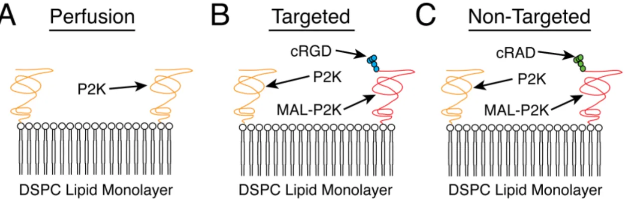
MCAs for perfusion-based experiments were created using a 9:1 molar ratio of 1,2 Distearoyl - sn - Glycero - 3 - Phosphocholine (DSPC) (Avanti Polar Lipids, Alabaster, AL) and 1,2 Distearoyl - sn - Glycero - 3 - Phosphoethanolmine - N - Methoxy - PEG - 2000 (P2K) (Avanti Polar Lipids - Alabaster, AL) in a 90 mL buffer solution (Figure 4.2A). The buffer solution was comprised of 80% phosphate buffered saline (PBS), 15% propylene glycol and 5% glycerol and the final lipid concentration was 1.0 mLmg.
4.3.2 Non-targeted Agent Recipe
Non-targeted (control) lipid solutions for molecular imaging experiments were created using DSPC, P2K, and 1,2 Distearoyl sn Glycero 3 Phosphoethanolamine N -Maleimide (PEG)-2000 (MAL-P2K) cross-linked to a cRAD peptide (Cyclo-Arg-Ala-Asp-D-Tyr-Cys) in a 18:1:1 molar ratio respectively with a total lipid concentration of 1.0 mLmg. Finally, the lipids were suspended in 90 mL of sterile PBS (Figure 4.2C).
4.3.3 Targeted Agent Recipe
Microbubbles designed to targetαvβ3 integrins for molecular imaging experiments were
(Figure 4.2B). Similar to the perfusion and non-targeted agents, lipids were fabricated with a total lipid concentration of 1.0 mLmg in a 90 mL buffer solution of sterile PBS. The chosen cRGD peptide has previously been shown to targetαvβ3-expressing vasculature,
which is characteristic of angiogenic tumors [22; 38; 81].
Figure 4.2: Illustrations of the various microbubble architectures used in this disserta-tion. A: Perfusion-based microbubble architecture consisting of a DSPC lipid monolayer and a P2K brush layer. B: Targeted microbubble architecture consisting of a DSPC lipid monolayer, a P2K brush layer, and a cRGD peptide linked to a MAL-P2K. C: Non-Targeted microbubble architecture consisting of a DSPC lipid monolayer, a P2K brush layer, and a cRAD peptide linked to a MAL-P2K.
4.3.4 Lipid Preparation Procedure
Briefly, powdered lipids were measured to precise weights using a high precision bal-ance (AB204-S, Mettler Toledo, Greifensee, Switzerland) with the previously described recipes. The lipids were placed into a 100 mL glass vial with 2 mL of chloroform, an organic compound in which lipids easily dissolve. Next, the lipids were thoroughly agitated with a vortex mixer until all lipids were visibly dissolved in the chloroform. Then, the chloroform was evaporated in the presence of slow-flowing nitrogen and si-multaneous agitation with the vortex mixer. After the chloroform was removed from the container, the dried lipids were added to an oven, under vacuum, at 55◦C for 30 minutes to remove any remaining chloroform from the container. Finally, the buffer
solution was added to the lipid container and introduced to a sonication (Branson 2510, Branson Ultrasonics, Danbury, CT) bath for 30 minutes at 55◦C for re-hydration.
4.3.5 Unsorted Microbubble Populations
Unsorted microbubbles were produced using mechanical agitation, which is the fabri-cation method that is utilized for the FDA - approved contrast agent DefinityR. First, 1.5 mL of the appropriate lipid solution was transferred to a 3 mL serum vial. The vial was stoppered and capped and decafluorobutane was exchanged with the air in the vial headspace using a custom vacuum apparatus. The vial was shaken vigorously for 45 seconds at 4500 rotations per minute using a mixer (Vialmix, Bristol-Myers Squibb Medical Imaging, North Billerica, MA) to produce the characteristic polydisperse dis-tribution for perfusion-based in vivo experiments.
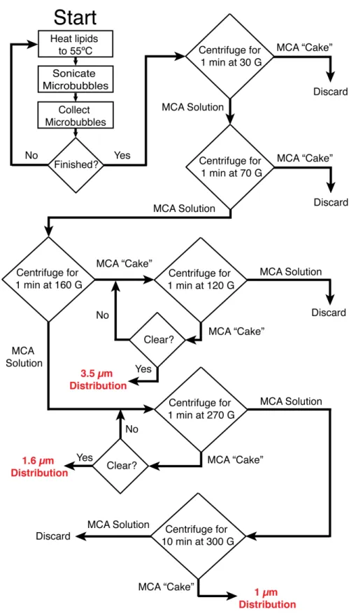
4.3.6 Sorted Microbubble Populations
The specific procedure for sorting microbubbles is presented in this section as an item-ized list of steps and as a flow chart in Figure 4.4. The method used to create various size distributions is based on differences in buoyancy forces for different microbubble sizes and was recently described in detail by Feshitan and colleagues [41]. Using this technique, sorted distributions with mean diameters of ∼1.0 µm, ∼1.6 µm, and ∼3.5 µm may be obtained (Figure 4.3). It is important to note that the mode of the
Microbubble Production
A large quantity of lipid solution is required (typically 90 mL or more at a minimum concentration of 1.0 mLmg) to yield the appropriate number of sorted microbubbles. This lipid solution is prepared via the methods described in section 4.3.4. After the lipid solution is prepared, different diameter distributions are preferentially selected using a multi-step centrifugation procedure as follows:
1. Lipids are completely dissolved in the buffer solution by raising the solution tem-perature to 55◦C.
2. The beaker of lipids is transferred to the sonic dismembrator apparatus. The sonicator tip is placed such that it is ∼1 mm below the surface of the lipid solution.
3. The sonic dismembrator is set to a power of 70% and a time of 15 seconds.
4. A large collection of microbubbles is generated via acoustic emulsification by turning the sonicator on while flowing decafluorobutane over the surface of the solution.
5. The resulting microbubbles (in solution) are collected using 30 mL syringes.
6. The 30 mL syringes are placed in a centrifuge for 10 minutes at 300 G.
7. After 10 minutes, a microbubble “cake” forms toward the plunger of the syringe. The buffer solution is slowly pushed out of the syringe (everything but the mi-crobubble “cake”) into a beaker for recycling.
8. Approximately 1 mL of buffer solution is added to the syringe containing the microbubble “cake” for every 1 mL of microbubbles produced.
9. Using the recycled lipid solution, steps 1 through 8 are repeated until at least 30 mL of microbubbles have been collected.
3.5 Micron Diameter Isolation
1. The well-mixed 30 mL syringe of microbubbles is placed into a centrifuge for 1 min at 30 G.
2. The resulting microbubble solution is slowly pushed out into another 30 mL syringe and the microbubble “cake” is discarded.
3. Filtered PBS is added to the syringe containing the solution until there is a final volume of 30 mL.
4. The 30 mL syringe of microbubbles is placed into a centrifuge for 1 min at 70 G.
5. The resulting microbubble solution is slowly pushed out into another 30 mL syringe and the microbubble “cake” is discarded.
6. Filtered PBS is added to the syringe containing the solution until there is a final volume of 30 mL.
7. The 30 mL syringe of microbubbles is placed into a centrifuge for 1 min at 160 G.
8. The resulting microbubble solution is slowly pushed out into another 30 mL syringe for ∼1.0 µm and ∼1.6 µm selection.
9. The “cake” is transferred to a 5 mL syringe for the selection of∼3.5 µm diameter microbubbles.
10. Filtered PBS is added to the syringe until there is a final volume of 5 mL.
12. The resultant microbubble solution is slowly pushed out of the syringe while the microbubble “cake” is retained.
13. Steps 10 through 12 are repeated until the resultant solution is completely clear.
14. The final microbubble population is stored in a 3 mL syringe with no headspace. The size distribution is described in Figure 4.3C.
1.6 Micron Diameter Isolation
1. Using the resultant microbubble solution from step 8 above, the 30 mL syringe is placed in the centrifuge for 1 min at 270 G.
2. The resulting microbubble solution is slowly pushed out into another 30 mL syringe for ∼1.0 µm size-selection.
3. Filtered PBS is added to the syringe containing the microbubble “cake” until there is a final volume of 30 mL.
4. The 30 mL syringe is placed in the centrifuge for 1 min at 270 G.
5. The resultant microbubble solution is slowly pushed out of the syringe and dis-carded while the microbubble “cake” is retained.
6. Steps 3 through 5 are repeated until the resultant solution is completely clear.
7. The final microbubble population is stored in a 3 mL syringe with no headspace. The size distribution is described in Figure 4.3B.
1.0 Micron Diameter Isolation
1. Using the resultant microbubble solution from step 2 above, the 30 mL syringe is placed in the centrifuge for 10 min at 300 G.
2. The resulting microbubble solution is slowly pushed out and discarded.
CHAPTER 5
Imaging and Animal Preparation
5.1 Imaging Contrast Agents
Lipid-encapsulated microbubbles oscillate in the presence of an acoustic wave [36; 82]. When a microbubble is insonified, it expands and contracts in rhythm with the negative and positive pressure half cycles respectively. In general, the microbubble is analogous to a spring-mass system where the balance of forces are governed by the restoring force of the encapsulated gas and the inertia of the surrounding fluid pushing on the shell surface [36].
5.1.1 Amplitude Modulation Imaging Overview
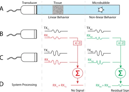
Amplitude modulation is a contrast agent imaging technique that utilizes the depen-dence of the microbubble response on the amplitude of the transmitted pulse [36; 84]. A brief and generalized description of this technique is provided in this section (Figure 5.1). First, two different interrogation pulses are transmitted with different amplitudes, but with the same frequency [36; 84]. Typically, the second pulse has an amplitude that is twice the amplitude of the first pulse [36; 84]. The imaging system then stores the backscattered intensity from the interrogated region for each of the two pulses. Post-processing is then performed on the two signals. The first stored echo is multiplied by a factor of two before it is subtracted from the second stored echo sequence [36; 84]. This technique has two different outcomes for linear scatterers and non-linear scatterers. For linear scatterers, or stationary tissue (at low pressure amplitudes), the second echo will be equivalent to two times the first echo; therefore, the final subtracted signal will equate to a zero value. In other words, the two-pulse technique will ultimately produce zero signal for linear or tissue-like scatterers. For non-linear scatterers, however, echoes produced by the two pulses will not subtract to zero. The residual signal created after post-processing represents the non-linear signal produced by the interrogated MCAs. The one disadvantage of this technique over conventional b-mode imaging is that the frame rate is sacrificed due to the requirement of multiple transmit pulses, which may sacrifice our ability to detect fast moving objects with this technique.
5.1.2 Pulse Inversion Imaging Overview
Figure 5.1: High-level description of the amplitude modulation imaging technique. A: Pictorial description of the setup to describe amplitude modulation. In this panel a transducer interrogates both a tissue region and a microbubble region. At low pressure amplitudes, the tissue will behave as a linear target and the microbubble will behave non-linearly. B: A two-cycle pulse is transmitted at amplitude A and the return echo is stored for both tissue and microbubbles. C: Again, a two-cycle pulse is transmitted only this time the amplitude of the signal is 2A. The return echo is stored for both tissue and microbubbles. D: The receive signal from the first pulse sequence is multiplied by minus two and then added to the second receive signal. The final result for the tissue region will be zero whereas the result for the microbubble region will equate to a non-zero value.
Then, another two-cycle pulse is transmitted only this time it is inverted relative to the initial transmitted pulse [36; 85; 82]. The echo from the inverted signal is stored and is added to the received signal from the initial pulse [36; 85; 82]. Due to the non-linearity of microbubbles, the echo from the inverted pulse will differ from echo from the initial pulse, which will sum to a non-zero value. The linear scatterers, however, will behave the same for both the first and inverted pulses and thus sum to zero.
Figure 5.2: High-level description of the pulse inversion imaging technique. A: Pictorial description of the setup to describe pulse inversion. In this panel, a transducer inter-rogates both a tissue region and a microbubble region. At low pressure amplitudes, the tissue will behave as a linear target and the microbubble will behave non-linearly. B: A two-cycle pulse is transmitted and the return echo is stored for both tissue and microbubbles. C: Again, a two-cycle pulse is transmitted only this time the signal is inverted from B. The return echo is stored for both tissue and microbubbles. D: The two receive signals for tissue are summed and equate to zero. The two microbubbles, being non-linear, sum to a non-zero value.
5.1.3 CPS Imaging Overview
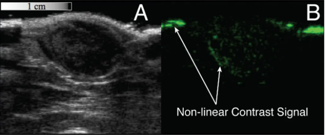
much more complex in its implementation [36; 86].
Figure 5.3: Examples of both b-mode and CPS images output from the Siemens Sequoia system. A: The grayscale b-mode image is a typical anatomical interrogation of a subcutaneous fibrosarcoma tumor. B: An interrogation of the same tumor in the same location, but using CPS mode, a non-destructive non-linear imaging technique, which suppresses the signal from the tissue. The green signal is the receive signal from non-linear targeted microbubbles within the tumor tissue.
5.1.4 Harmonic and Sub-Harmonic Imaging Overview
As previously mentioned, microbubbles behave similar to a spring-mass system [36]. Moreover, the oscillatory motion of the microbubble in an acoustic field may contain harmonic and sub-harmonic energies relative to the fundamental transmit frequency, f0 [82]. By utilizing these properties, it is possible to detect microbubbles through
harmonic and sub-harmonic imaging techniques [82; 87; 88].
Harmonic imaging is a method where the ultrasound system separates the second harmonic frequency signal from the fundamental transmit frequency. Briefly, an ultra-sound system generates a transmit pulse at a frequency f0 that is within the bandwidth
of the system. The microbubble oscillates and produces harmonic energies, which are subsequently detected by the system at the second harmonic frequency, 2f0 [36; 82].
By using filtering techniques, the harmonic signals are separated from the fundamental
frequency, which contains most of the energy detected from tissue. Unfortunately, at high enough pressures, tissue may also generate harmonic signals [36; 82]. Therefore, most of the systems that incorporate this technique are obscured by residual tissue signal components, which cannot be completely separated from the microbubble signal [36; 82]. Since this is not a multi-pulse imaging strategy, frame-rates are typically not compromised when using this technique.
Under certain conditions, microbubble contrast agents also generate sub-harmonic energy [87; 88; 89]. Sub-harmonic imaging is a technique that utilizes this behavior as a means to separate the microbubble signal from the tissue signal. Sub-harmonic imaging is similar to harmonic imaging; however in this detection scheme, the ultra-sound system receives the scattered microbubble signal at 12f0, rather than twice the
fundamental frequency [87; 88; 89]. Since the received signal is lower in frequency than the fundamental, this technique does not suffer significantly from frequency-dependent attenuation. Unfortunately, the resolution of the system worsens because of the lower detected sub-harmonic frequencies. Similar to harmonic imaging, frame-rates are typi-cally not affected when using this technique due to its single-pulse strategy.
While harmonic imaging and sub-harmonic imaging have been utilized successfully in various applications, these imaging techniques were not inherent to our clinical ul-trasound system, and thus not available as a comparison to CPS. Therefore, allin vivo imaging throughout this dissertation was performed using CPS imaging.
5.2 Experimental Methods - Imaging System 5.2.1 System overview and capabilities
regions of interest for quantifying biomarker expression within a tumor. Thus, for all experiments performed, b-mode US images of tumors were taken at 14 MHz in spatial compounding mode. Another necessary component for quantifying biomarker expression in molecular imaging experiments is the destruction of microbubbles. This was achieved using the D Color function (Color Doppler) at 7 MHz with a maximum mechanical index (MI) of 1.9. Prior studies utilizing a MI of 1.9 to destroy microbubbles suggest no indication of bioeffects when higher frequencies (≥7 MHz) are utilized [90].
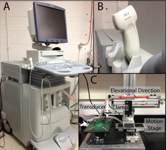
Figure 5.4: Images of the US scanner used for all of the studies described herein. A: Siemens Acuson Sequoia with a 15L8 linear array transducer. B: Close-up of the 15L8 linear array transducer that was used in all US experiments. C: 3-D stage used for all volumetric acquisitions. The transducer was positioned in a fixed clamp and digitally stepped in the elevational direction using the linear motion stage shown in the image.
5.2.2 Experimental Methods - CPS Imaging
MCAs were imaged in CPS mode, which is a non-destructive contrast-specific imaging technique previously described in 5.1.3. CPS was implemented to provide a high con-trast to tissue ratio while being minimally destructive to microbubbles [56; 60; 86]. For all contrast imaging, the transducer was operating at a frequency of 7 MHz and a MI of 0.18 with a dynamic range of 80 dB. In a preliminary experiment, the video intensity of targeted agents in vivo was observed over 30 seconds using CPS at a MI of 0.18. In this experiment (data not shown), no loss in signal intensity was observed over the evaluated time frame, indicating that our imaging parameters were non-destructive. This conclusion was corroborated by Kaufmann and colleagues in a study performed in 2010 evaluating the effect of power on microbubble adherence in molecular imaging experiments in vivo [91].
5.2.3 Experimental Methods - 3-D Imaging Apparatus
To create 3-D data sets, the transducer was positioned in a fixed clamp and digitally stepped in the elevational direction using a linear motion stage (Model UTS150PP, Newport Irvine, CA) (Figure 5.4C). A custom LabView (National Instruments Austin, TX) program was interfaced to both the motion stage and the US system. Using output signals from the US system, the step-size of the motion stage was precisely positioned while simultaneously triggering the capture of video data at every discrete step [81; 92]. The elevational beam width of the 15L8 transducer was calculated to be ∼800 µm.
5.2.4 Experimental Methods - ARF for MCA Translation
duty cycle with a pulse repetition frequency (PRF) of 25 kHz. The axial focus was positioned deep into tissue (∼6 cm) to create an unfocused application of ARF. Finally, the amplitude of the ARF pulses was modulated by using the power output dial of the US system.
5.3 Animal Preparation and MCA Administration
In this section, we describe how animals were prepared and contrast agents were ad-ministered for the studies in Chapters 7 through 11. All animal studies were conducted in accordance with the protocols approved by the University of North Carolina School of Medicine’s Institutional Animal Care and Use Committee.
In Chapters 7 through 11, rats of similar sizes (∼125 g) were used for all in vivo studies. The tumor model used in allin vivo experiments was a rat fibrosarcoma (FSA) [93]. In previous studies, this particular type of tumor has been shown to provide a good model for αvβ3 targeted molecular imaging [38; 81]. It should be noted, however,
that an R3230 mammary carcinoma tumor model was also evaluated in Chapter 8.
5.3.1 Tissue Implantation
During the tumor tissue implantation procedure, the rats were anesthetized using 2% inhaled isoflurane mixed with oxygen. The animal’s body temperature was maintained at 37◦through the use of a temperature-controlled heating pad. Next, the rat’s left flank was shaved and disinfected and a 2 mm incision was made above the quadriceps muscle. Finally, a small 1 mm3 piece of tumor tissue was positioned subcutaneously and allowed
to grow for approximately 2 weeks. Once the tumor had grown to approximately 1 cm in diameter in the longest measurable axis, imaging was performed.
5.3.2 Animal Preparation for Imaging
Rodents were anesthetized with 2% inhaled isoflurane mixed with oxygen. Once the rat was sedated, the area to be imaged was shaved with small animal hair clippers and further depilated using a chemical hair remover. A 24-gauge catheter was inserted into the tail vein of the animal for the purpose of administering MCAs. The US transducer used in thein vivo analysis was positioned in a fixed clamp and coupled to the animal with US gel. Throughout the imaging procedure, the rodent’s body temperature was maintained through the use of a temperature-controlled heating pad .
5.3.3 Contrast Administration
The sizes and concentrations of stock solutions for all microbubble types used in all studies were measured prior to each imaging study using an Accusizer 780A laser light obscuration and scattering device (Particle Sizing Systems, Santa Barbara, CA, USA). For each injection, the appropriate volume of stock solution was added to the catheter via a micropipette tip and flushed with sterile saline. Animals received less than 1.5 mL limit of total fluid volume through the tail vein within any 24-hour period.
Table 5.1: Summary of Animal Study Parameters
Chapter Animal # Animals Imaging Tumor Imaging
Type Subject Type Type
7 Rat 13 Tumor FSA MI
8 Rat 9 Kidney NA Perfusion
8 Rat 3 Tumor FSA, R3230 MI
9 Rat 8 Tumor FSA MI
10 Rat 8 Tumor FSA MI
11 Rat 8 Tumor FSA MI
11 Rat 8 Tumor FSA Perfusion
12 Mouse 14 Tumor Panc. DCE-PI
12 Mouse 14 Tumor Panc. MI
CHAPTER 6
Experimental Diagnostic Methods
This chapter describes the experimental diagnostic procedures utilized in this disser-tation. Each section generally describes the method, how the data was obtained from each method and its implementation herein.
6.1 Perfusion-Based Imaging and Methods
6.1.1 Time-Intensity
In this dissertation, microbubble clearance from the circulatory system was measured in vivo by observing the length of time that each type of microbubble persisted in the tumor vasculature (or kidney in Chapter 8) after a bolus injection of MCAs. Briefly, the linear array transducer was placed in a fixed clamp to maintain the same imaging plane and the imaging system was set to a center frequency of 7 MHz in CPS mode. After each bolus injection, the MCA wash-in was recorded at a 1 Hz sample rate using the clip store function on the US system. Once there were no microbubbles visibly moving in the vasculature, the video was stopped and analyzed offline. Figure 6.1 describes the procedure of measuring the intensity of a region of interest over time for the purposes of evaluating microbubble clearance.
Figure 6.1: Diagram that describes the mechanism for obtaining a time-intensity curve for contrast-enhanced imaging. Persistence is measured as the time from the peak intensity to the time that the video intensity of the ROI reached half of the peak intensity.
Of note, only animal studies with contrast administration not requiring radiation force were used to collect persistence data, because the volumetric administration of
ARF interferes with our ability to observe the contrast agent wash-in. This is directly related to data that was collected in Chapter 11.
6.1.2 Destruction-Reperfusion
Dynamic contrast-enhanced perfusion imaging (DCE-PI) is an US technique that is used to non-invasively monitor the blood flow in both large vessels and in the capil-lary microcirculation using non-targeted perfusion-based MCAs. This technique uses a short, high-intensity pulse of US that causes rapid destruction of MCAs in the in-terrogated region. This clearance pulse is immediately followed by a low-intensity contrast-specific signal that does not fracture the microbubbles, but instead allows for the pixel-by-pixel observation of blood flow rates as the MCAs enter back into the tissue [71; 96]. Accordingly, changes in contrast enhancement over time can provide information about tissue perfusion. Figure 6.3 illustrates the concept of DCE-PI.
Figure 6.3: Diagram describing the destruction-reperfusion approach to DCE-PI. MCAs are destroyed and subsequently interrogated until the intensity reaches 20% of the maximum.