UNCSTUDY_CC.pdf

(1)

Evaluating the impacts of the clean cities program

Shiyong Qiu

a,

⁎

, Nikhil Kaza

b

a_{World Resources Institute China Ofﬁce, Room K-M, 7/F, Tower A, Donghuan Plaza, No. 9 Dongzhong Street, Dongcheng District, Beijing 100027, China} b

Dept. of City & Regional Planning, University of North Carolina at Chapel Hill, 110 New East, Campus Box 3140, Chapel Hill, N.C. 27599-3140, United States

H I G H L I G H T S

•The clean cities program is effective in promoting alternative fueling stations. •The program has potentially shifted

travel behaviors from driving to riding transit.

•Counties in the program experienced larger improvements in air quality. •In these counties, fewer commuters

drive to work and more use transit.

G R A P H I C A L A B S T R A C T

a b s t r a c t

a r t i c l e i n f o

Article history: Received 20 June 2016

Received in revised form 17 November 2016 Accepted 17 November 2016

Available online 25 November 2016

Editor: D. Barcelo

The Department of Energy's Clean Cities program was created in 1993 to reduce petroleum usage in the transpor-tation sector. The program promotes alternative fuels such as biofuels and fuel-saving strategies such as idle re-duction andfleet management through coalitions of local government, non-profit, and private actors. Few studies have evaluated the impact of the program because of its complexity that include interrelated strategies of grants, education and training and diversity of participants. This paper uses a Difference-in-Differences (DiD) approach to evaluate the effectiveness of the program between 1990 and 2010. We quantify the effectiveness of the Clean Cities program by focusing on performance measures such as air quality, number of alternative fueling stations, private vehicle occupancy and transit ridership. Wefind that counties that participate in the program perform better on all these measures compared to counties that did not participate. Compared to the control group, counties in the Clean Cities program experienced a reduction in days with bad air quality (3.7%), a decrease in automobile commuters (2.9%), an overall increase in transit commuters (2.1%) and had greater numbers of new alternative fueling stations (12.9). The results suggest that the program is a qualified success.

Alternative fuel vehicles Air quality

Vehicle miles traveled Policy evaluation

1. Introduction

The transportation sector contributes about 50% of all smog-forming volatile organic compounds (VOCs), nitrogen oxide (NOx) emissions, and toxic air pollutant emissions, and about 75% of all carbon monoxide ⁎ Corresponding author.

E-mail addresses:[email protected](S. Qiu),[email protected](N. Kaza).

Contents lists available atScienceDirect

Science of the Total Environment

(2)

(CO) emissions in the U.S. (United States Environmental Protection Agency, 2007). Petroleum-based products such as gasoline and diesel account for much of this pollution. Federal policies have focused on re-ducing petroleum consumption in the transportation sector by promot-ing alternative fuels, reducpromot-ing vehicle miles traveled (VMT) and increasing fuel ef_ficiency of automobiles (Congress of the United States & Congressional Budget Office, 2002; Gallagher et al., 2007; Knittel, 2012). Part of this effort is supported by the Department of Energy’s Clean Cities program, which promotes petroleum reduction in American cities. Created by the U.S. Department of Energy (DOE) in 1993, the Clean Cities program aims to reduce petroleum consumption in transportation through alternative and renewable fuels, fuel econo-my improvements, idle reduction, and other fuel-saving technologies and practices (United States Department of Energy, Energy Efficiency & Renewable Energy, 2016a). Clean Cities Coalitions (CCCs) are public-private partnerships comprised of businesses, fuel providers, state and local agencies, and community organizations (United States Department of Energy, Energy Efficiency & Renewable Energy, 2016a). Because the program is complex and consists of interrelated pollution mitigation strategies, evaluation has hitherto relied on accounting for displaced petroleum consumption from alternative fuelfleet adoptions and mitigation factors associated with strategies such as idle reduction (United States Department of Energy, Energy Efficiency & Renewable Energy, 2016b). Little is known about the impact of the program on air quality or petroleum demand reduction as data are hard to obtain and establishing causal relationships is challenging.

This study provides an initial characterization of efﬁcacy of the Clean Cities program. The program's impacts are evaluated by comparing the difference in various outcome measures between counties located in-side and outin-side the boundaries of CCCs between 1990 and 2010, while controlling for meteorological, sociological, and demographic fac-tors. We focus on different outcome measures such as air quality, alter-native fuel use, commuters using automobile and transit. Weﬁnd that the Clean Cities program is positively associated with a decrease in the number of days with bad air quality. Moreover, counties that are part of CCCs have more alternative fueling stations than counties that are not. Finally, our results suggest that the Clean Cities program discour-ages driving to work and encourdiscour-ages transit ridership, potentially yield-ing a reduction in transportation-related air pollution.

2. Background

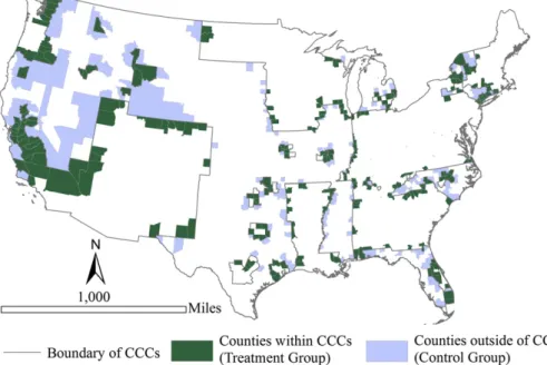
The 1992 Energy Policy Act required certain vehiclefleets (e.g. feder-al and statefleets in metropolitan areas excluding emergency and law enforcement) to acquire Alternative Fuel Vehicles (AFVs). The DOE established the Clean Cities program in 1993 to provide resources to thesefleets and other voluntary adopters (United States Department of Energy, Energy Efficiency & Renewable Energy, 2016a). The program provides resources and information to help transportation stakeholders evaluate options and achieve goals related to alternative fuels, advanced vehicle technologies, and other strategies to curtail petroleum use. A formal designation occurs when a local champion, such as a county gov-ernment, local non-profit, or city agency working with the DOE, assem-bles local stakeholders and develops a program plan for the coalition. The local coalitions provide opportunities for transportation stake-holders to coordinate their actions with one another to reduce petro-leum use. CCC designation occurs on voluntary basis; however, the coalition has the capacity to identify a healthy marketplace for alterna-tive fuels and other petroleum reduction strategies, establish a clear or-ganizational structure, and maintain strong partnerships with relevant government departments (United States Department of Energy, 2016). The designation process can take anywhere from one to three years. When the Clean Cities program commenced, six local coalitions were formed (United States Department of Energy, 2016) and by mid-2016, this number grew to 84 CCCs nationwide, encompassing more than half of all U.S. counties (seeFig. 1) (United States Department of

Energy, Energy Efficiency & Renewable Energy, 2016c). The central aim of the Clean Cities program is to decrease petroleum consumption in the U.S. by 2.5 billion gal per year by 2020 (United States Department of Energy, Energy Efficiency & Renewable Energy, 2016b). The Clean Cities program aims to build partnerships among state and local actors within both the public and private sectors to overcome crit-ical barriers that have impeded the acquisition of AFVs and use of alter-native motor fuels. These barriers include the low price of gasoline and diesel, insufficient availability of alternative fuel refueling infrastruc-ture, and the relatively high cost of AFVs (Santini et al., 1995; Whalen et al., 1999; Rubin & Leiby, 2000). The program's main strategies are 1) to encourage a voluntary approach to AFV development and acquisi-tion; 2) to implement and oversee major activities such as grants for in-stallation of idle-reduction technologies and technical training through local designated coordinators; 3) to pay attention to niche markets, such as airport, transit, and government_fleets; 4) to enable and encourage development of refueling infrastructure; 5) to involve federal and state governments in developing and supplying funding, information resources, and technical assistance (Zhao & Melaina, 2006).

In 2013 alone, the Clean Cities program claims to have saved about 1 billion gal of petroleum through alternative fuels and vehicles (70.5%), increased adoption of electric vehicles (13.7%), reductions in VMT (6.7%), idle reduction (5.3%), and improved fuel economy (2.8%) (United States Department of Energy, Energy Efﬁciency & Renewable Energy, 2016b), which is equivalent to preventing 5.7 million tons of Greenhouse Gas (GHG) emissions (Johnson & Singer, 2014). However, these effects are estimated through simulations based on tools devel-oped by Argonne National Labs (e.g. GREET Model, the Greenhouse Gases, Regulated Emissions, and Energy Use in Transportation Model). Evaluations of other outcomes, such as air quality improvements, are scant in the literature.

Studies have found that alternative fuels differ in their advantages and disadvantages for air quality compared to petroleum (Lave et al., 2000; Schell et al., 2002; Frey et al., 2009a). For example, biodiesel can reduce particulate matter (PM), CO and total hydrocarbon (HC) emis-sions signiﬁcantly (Haas et al., 2001; Morris & Jia, 2003; McCormick, 2007; Lapuerta et al., 2008; Janaun & Ellis, 2010), but may increase NOxemissions upwards of 80% compared to petroleum diesel (Haas et

al., 2001; Hansen et al., 2006). Electric vehicles are able to eliminate emissions of CO and HC and greatly reduce NOx emissions, while they are reported to increase emissions of sulfur oxide (SOx) and PM (DeLuchi et al., 1989; Wang & Santini, 1992; Lave et al., 1995; Jacobson et al., 2005; Brady & O'Mahony, 2011). Although propane is found to increase mercury (Hg) emissions (Won et al., 2007), it has the potential to decrease the emissions of Ozone (O3), PM, NOx, CO, and HC (Chang et al., 2001; Ristovski et al., 2005). Additionally, the air quality beneﬁts of alternative fuels such as ethanol (Knapp et al., 1998; Hsieh et al., 2002; Niven, 2005; Anderson, 2009) and natural gas (Goyal, 2003; Ravindra et al., 2006) are still under debate. CCCs pro-mote a range of alternative fuels that suit regional and local needs. For these reasons, it is more appropriate to evaluate the attendant air qual-ity beneﬁts of a comprehensive alternative fuels program broadly, rath-er than evaluating the effects of individual fuels separately.

(3)

Transportation Efﬁciency Act, and the Transportation Equity Act (United States Department of Transportation & Federal Highway Administration, Policy and Government Affairs, 2014). Thus, the effect of CCCs should be evaluated through analyzing a more comprehensive list of indicators rather than simply modeling potential petroleum substitution.

3. Materials and Methods

3.1. Outcome measures

To evaluate the impact of CCCs, we measure the difference in the number of days with bad air quality in counties within and outside of the CCCs. If the CCCs are effective, counties within the coalitions should have signiﬁcantly lower numbers of days with poor air quality com-pared to counties outside of them. We choose Air Quality Index (AQI) as the measurement of overall air quality, which can be acquired from the AirData Air Quality Index Summary Report published by U.S. Envi-ronmental Protection Agency (EPA) since 1980 (United States Environmental Protection Agency, 2016). AQI considers all of the criteria air pollutants within a geographic area based on the National Ambient Air Quality Standards (NAAQS). The index ranges from 0 to 500; an AQI value above 100 is considered to be unhealthy from a public health perspective (AirNow, 2016; U.S. Environmental Protection Agency, 2014). We use the maximum daily AQI value to account for multiple monitoring stations within a county, and then count the num-ber of days where AQI was above 100 in that year (McCarty & Kaza, 2015). We calculate the proportion of days with an AQI above 100 and average the proportion between 1980 and 1982, between 1988 and 1992, and between 2008 and 2012. This method averages out the effect of exceptional events (e.g. forestﬁres) that might contribute to a higher proportion of AQI in a particular year.

The differences in air quality can be attributed to either alternative fuels strategy or VMT reduction strategy or both. To measure whether the alternative fuel strategy is effective, we use the number of alterna-tive fueling stations in the county as an indicator. However, such a direct indicator is not readily available for the VMT reduction strategy because VMT data are not consistently available at a sub-metropolitan level. In-stead, we use two outcome variables, private vehicle occupancy (% of commuters using car) and transit ridership (% of commuters using

transit), as proxies because they are shown to be associated with total VMT in an area (Carlson & Howard, 2010; Holtzclaw, 1991; McMullen & Eckstein, 2013).

We acquired data on alternative fueling stations from the U.S. DOE Energy Efficiency and Renewable Energy Alternative Fuels Data Center (United States Department of Energy, Energy Ef_ficiency and Renewable Energy, 2015). Stations include all alternative fuels and both existing private and public stations. Since alternative fueling sta-tion data include the specific address of the station and corresponding ZIP Code instead of the Federal Information Processing Standard (FIPS) county code, we used the 2010 ZIP Code Tabulation Area to County Re-lationship File provided by the U.S. Census Bureau to assess the number of stations within each county.

Data on private vehicle occupancy and means of transportation to work come from the U.S. Decennial Census 1980 (United States Census Bureau, 1980), 1990 (United States Census Bureau, 1990) and American Community Survey 2008–2012 (5-Year Estimates) (United States Census Bureau, 2012).

3.2. Control variables

Average daily maximum air temperatures in the years of 1980, 1990 and 2010 were acquired at the county level from the North America Land Data Assimilation System (Centers for Disease Control and Prevention, 2016). Data on other covariates including total population, urban population, unemployment rate for total population 16 years and over, workers in manufacturing and construction (NAICS codes 31-33 & 21), median household income, and time for workers travelling to work are from the U.S. Decennial Census 1980 (United States Census Bureau, 1980), 1990 (United States Census Bureau, 1990) and American Community Survey 2008–2012 (5-Year Estimates) (United States Census Bureau, 2012).

3.3. Research design

(4)

within CCCs that were designated between 1990 and 2010. Data on the CCCs are from the U.S. DOE Energy Efficiency and Renewable Energy Clean Cities of_ficial website. Sometimes the CCCs lose designation, or are“dedesignated”, due tofinancial difficulties or lack of support (United States Department of Energy, Energy Efficiency & Renewable Energy, 2016c). However, due to data limitations, this study does not take these dedesignated coalitions into account. The resulting sample includes 428 counties. Among them, 231 counties are within the CCCs (treatment group) and 197 counties are outside of them (control group) (Fig. 2).

We examine the effectiveness of the Clean Cities program using the Difference-in-Differences (DiD) approach, a common method for evalu-ating the effect of a policy intervention (Dimick & Ryan, 2014; Chemin & Wasmer, 2009; Ashenfelter, 1978; Heckman & Robb, 1985; Benmarhnia et al., 2016; Girma & Gorg, 2007; Angrist & Pischke, 2008; Chang et al., 2016). The DiD method uses a comparison group that is experiencing similar trends but has not received the policy intervention and com-pares outcome measures for both the treated group and the untreated (comparison) group before and after the policy intervention. The DiD estimator measures the differenceð^δÞbetween the difference in average outcome in the treatment group before and after the policy intervention and the difference in average outcome in the control group over the same time period. Mathematically,

^ δ̂ ¼ Ycccafter−Y

ccc before

− Ynonafter−ccc−Y non−ccc before

ð1Þ

where Y is the average outcome. Therefore, there are four groups in this model: pre-treatment treated, pre-treatment control, post-treatment treated, and post-treatment control. Among these four groups, only the post-treatment treated group receives the intervention (i.e. Yafterccc in Eq.(1). The DiD estimator and this research design have the potential to eliminate threats to validity. For example, if automobile technology is concurrently improving with the CCC program but is unobservable, the researcher can falsely attribute the changes in air quality to the intervention.

We use a regression model to calculate the DiD estimator. The re-gression model can easily yield the DiD estimator and standard errors, and allow for the inclusion of additional covariates at the county level to reduce the residual variance and the effect of confounders

(Koppensteiner, 2013; Albouy, 2004). We use separate models for four different outcomes of interest: proportion of bad air quality days, num-ber of alternative fueling stations, private vehicle occupancy and transit ridership.

IfYitis the outcome variable of interest, e.g. proportion of bad air quality days in periodtand countyi, then the regression model is spec-iﬁed as:

Yit¼β0þβ1Xiþβ2Kiþβ3Ttþβ4ðXiTtÞ þβj Zjþμit ð2Þ

whereXiis a dummy variable equal to 1 if the county is located inside the boundaries of a CCC (treatment group) and 0 if it is located outside the boundaries of a CCC (control group); Kidenotes the number of years since designation of the CCC; Ttis a dummy variable equal to 1 for 2010 data (post-treatment period) and 0 for 1990 data (pre-treatment peri-od); Xi* Ttis the interaction taking the value 1 only for the treatment group in the post-treatment period. Thereforeβ4is the DiD estimator of interest. A negative value forβ4indicates a decrease in the proportion of bad air quality days (i.e. an increase in air quality) in CCC counties compared to non-CCC counties, while a positive value might indicate an increase in alternative fueling stations. Zj(jN4) denotes other covar-iates andμitis the error term. All data management and statistical anal-yses were conducted in STATA SE software, version 12.

4. Results

4.1. Descriptive statistics

The unemployment rate is marginally lower in counties within CCCs, while the proportion of industrial employment is similar between counties within and outside of CCCs both in 1990 and 2000 (seeTable 1). However, the share of industrial employment has declined and the unemployment rate has increased in the two decades under study reﬂecting the national trend. Both groups have similar median house-hold incomes. This suggests that the economic structure of both groups is roughly similar. Furthermore, because these are generally outlying counties to metropolitan areas, they have similar proportions of com-muters with long commutes (60 min or more). This proportion, howev-er, has increased from 5% to 7% during the two decades indicating the rise of the‘mega commuters’(Rapino & Fields, 2013). These commuting

(5)

patterns have implications for air quality. The total population as well as the urban population of the counties within CCCs are, on average, great-er than counties that are not in CCCs. Urban populations rose at a fastgreat-er rate in the CCC counties than the non-CCC counties, though it is unclear if the urbanization rates have any effect on the designation of coalition status. All these indicators point to the parallel growth trends within both groups of these border counties and thus, make the groups compa-rable to test the effect of the coalitions.

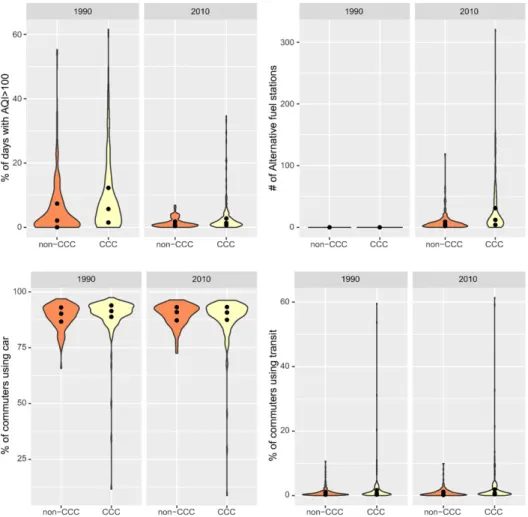
By comparing the differences in the outcome variables (Table 2and

Fig. 3), one can see that the air quality has improved throughout the na-tion between 1990 and 2010, while the effect is much more dramatic in CCC counties (α= 0.05). While there were no alternative fuel stations in the 1990s, there were many more in CCC counties than in neighbor-ing counties in 2010 (α= 0.01). The proportion of commuting by car, on average, increased in non-CCC counties, while it decreased in CCC counties. Furthermore, while the average proportion of transit com-muters declined in non-CCC counties, the proportion increased in CCC counties. The differences in proportion of transit commuters and auto commuters between the two groups of counties are not statistically signiﬁcant.

These descriptive statistics point to mixed success in outcome mea-sures of the coalitions. However, such conclusions are premature as these outcome measures could be inﬂuenced by changes in the control variables as well as larger technological and economic shifts across the study time period. The regression model accounts for these issues and contributes to a robust understanding of the effectiveness of the coali-tion designacoali-tion.

4.2. Parallel trends assumption

A central assumption of the DiD approach is the parallel trends as-sumption (Dimick & Ryan, 2014; Angrist & Pischke, 2008; Albouy,

2004), which states that the trends in outcomes between the treatment and control groups would be the same in the absence of the policy inter-vention. If this assumption is violated, the DiD estimator would be bi-ased due to different time trends in the control and treatment group. For example, if the two subsets of counties are inherently different in their air quality trajectories then the differences in air quality cannot be solely attributed to the CCC designation/participation. To address this issue, we focus only on counties that are located on the boundaries of CCCs. Neighboring counties, due to their spatial proximity, are ex-pected to share similar growth trajectories, thus ensuring that the char-acteristics of the treatment and control groups are comparable, aiming to eliminate as much observed heteroscedasticity as possible.

We test the parallel trend assumption by examining the significance of the coefficients in a regression model that uses data in the time period prior to the policy intervention. The term of interest is the interaction between the indicator variable representing whether the county belonged to CCC or not and the indicator variable representing the start (1980) and end (1990) of the period. Results indicate that there were no statistically significant differences in trends of the outcome measures between these two groups prior to the Clean Cities program (Table 3). Thus, the conclusions drawn in this study are robust.

4.3. Effect on air quality

The Clean Cities program designation is positively associated with a decrease in bad air quality days, the number of days where AQI is above 100 (Table 4). The difference in proportion of days with AQI_N100 be-tween the treatment and control groups has decreased signiﬁcantly since 1990 (α= 0.05). CCC counties experienced modest air quality im-provements (3.7 percentage points) compared to non-CCC counties and these improvements can be attributable to the CCC designation. The number of years of designation status of a CCC is positively associated Table 1

Descriptive statistics of covariates.

Variables 1990 2010

Not in CCC (n = 197) In CCC (n = 231) Not in CCC (n = 197) In CCC (n = 231)

Mean Std. dev. Mean Std. dev. Mean Std. dev. Mean Std. dev.

# of years since coalition designation 0 0 0 0 0 0 12.02 4.37

Population (000 s) 101.83 134.37 249.85 325.92 109.43 150.70 326.34 416.13

Proportion of urban population (%) 49.76 28.15 62.59 28.38 52.87 27.76 69.50 27.33

Unemployment rate (%) 7.08 2.53 6.33 2.06 9.60 3.24 9.30 3.06

Proportion of industrial employment (%) 25.12 10.24 26.08 8.87 17.80 6.02 18.17 5.69

Proportion of workers withN1 h commute (%) 4.94 3.13 5.30 3.74 6.58 3.91 6.79 4.21

Median household income (log) 10.67 0.22 10.77 0.25 10.69 0.22 10.8 0.23

California (yes/no) 0.14 0.12 0.12 0.11

Average daily maximum temperature (°F) 64.72 9.39 66.22 8.89 64.23 9.51 65.31 9.04

Table 2

Descriptive statistics of outcome variables.

Outcome variables and groups n 1990 2010 Difference between 1990 and 2010 DiD estimator

% days with AQIN100 (“bad”air quality)

In CCC 231 8.968 2.802 −6.166*** (0.726) −2.302** (1.101)

Not in CCC 197 5.230 1.366 −3.863*** (0.827)

Alternative fueling stations

In CCC 231 0 26.845 26.845*** (2.323) 18.611*** (3.522)

Not in CCC 197 0 8.234 8.234*** (2.647)

Commuters driving to work (%)

In CCC 231 89.814 88.155 −1.175 (0.765) −1.771 (1.159)

Not in CCC 197 89.155 89.751 0.596 (0.871)

Commuters using transit (%)

In CCC 231 2.176 2.469 0.293 (0.511) 0.367 (0.775)

Not in CCC 197 1.026 0.953 −0.074 (0.582)

(6)

with the proportion of days where AQIN100, though the relationship is not signiﬁcant. The model has modest predictive power (adjusted R2 ~0.218).

As expected, increase in the county population lead to increase in air pollution (α= 0.01). Since the difference in population between the treatment and control groups is even greater after the intervention, i.e. the treatment group has a greater population than the control group in 2010, the population difference between groups should not affect the direction and signi_ﬁcance of treatment effects. Similarly, increases in average daily maximum temperature, urbanization rate, and income all yield decreases in air quality, though the differences are not signiﬁ -cant. As expected, California counties experience more days with seri-ous air pollution issues (α= 0.01). Higher industrial employment (manufacturing and construction) is associated with worse air quality (α= 0.01). Unemployment rate, however, has a negative association with air quality (α= 0.05). This may be because: 1) unemployment rate tends to have lagged effect on air quality, 2) a higher unemploy-ment rate leads to more people looking for jobs, which could result in greater VMT, and 3) a higher unemployment rate does not necessarily mean lower industrial employment, which is observed to have a nega-tive relationship with air quality (McCarty & Kaza, 2015).

4.4. Impact on alternative fueling stations

The DiD estimates suggest that the Clean Cities program is associated with greater increase in the number of alternative fueling stations with-in the treatment counties compared to the comparison counties (α= 0.01, seeTable 4). CCC counties are expected to have 13 more alterna-tive fueling stations than non-CCC counties, on average. The estimates also suggest that counties with fewer alternative fueling stations are more likely to join the Clean Cities program (α= 0.01). This may be be-cause they can receive funding, information resources, and technical as-sistance through the program to build stations (Zhao & Melaina, 2006). This model has moderate predictive power (adjusted R2~0.543).

It should be noted that Californian counties, on average, are expected to have 6 more alternative fueling stations than other counties (α= 0.05). In addition to the CCC technical assistance, the state provides more incentives to encourage the construction of alternative fueling sta-tions such as AFV and Fueling Infrastructure Grants, and Natural Gas Ve-hicle (NGV) Home Fueling Infrastructure Incentive–South Coast. California's success story also provides evidence to support the symbio-sis between advocacy, education, and assymbio-sistance at different levels of governments and market actors (Zhao & Melaina, 2006).

Fig. 3.Distribution of the outcome variables.

Table 3

Results of pre-intervention trend.

Outcome variable

% days with AQIN100 Commuters driving to work (%) Commuters using transit (%)

DiD estimator 0.988 (2.418) 0.483 (1.160) −0.017 (0.807)

Adjusted R2 _0.191 _0.508 _0.538

(7)

4.5. VMT reduction

The difference in proportion of commuters driving to work between counties within CCCs and those outside of CCCs is 2.9 percentage points (_α= 0.05). This model has modest predictive power (adjusted R2 ~ 0.42). The Clean Cities program not only discourages private vehicle occupancy, but also encourages public transit ridership (α= 0.05), in-dicating its ef_ficacy on VMT reduction. CCC counties have experienced a 2.1 percentage point increase in transit ridership compared to non-CCC counties, on average. Nevertheless, the proportion of commuters riding transit has decreased as the number of years of CCC designation increases (α= 0.01). In other words, among those counties that take part in the program, the proportion of transit commuters decreases with time since coalition designation. This may be because the primary focus of the Clean Cities program has traditionally been on adopting al-ternative fuels, while promotion of public transit is a relatively novel ini-tiative (United States Department of Energy, Energy Efficiency & Renewable Energy, 2016b; United States Department of Energy, Energy Efficiency & Renewable Energy, 2016d). Coalitions who joined the program earlier may not be able to readily switch from a sole focus on alternative fuels to more varied projects like VMT reduction. Additionally, transit ridership is impacted by transit infrastructure im-provements and pricing. CCCs have limited influence over these large infrastructure and policy decisions. This model has modest predictive power (adjusted R2_~0.394).

In these models, unemployment rate has a signiﬁcantly negative as-sociation with transit ridership (α= 0.05). Unemployment rate also has a signiﬁcantly positive association with private vehicle occupancy (α= 0.01), which helps explain why the counties with higher unem-ployment rate have more bad air quality days.

5. Discussion

To date, the Clean Cities program has awarded over 400 million dol-lars towards various projects across the country to promote alternative fuels (United States Department of Energy, Energy Efﬁciency & Renewable Energy, 2016e). Thus, it is not surprising that alternative fuel stations have become more prevalent in counties contained within a coalition. Because there is very little publicly available disaggregate data about actual petroleum consumption, these stations are a proxy for the adoption of alternative fuelﬂeets and vehicles by organizations and households. However, the impact of AFV programs on air quality is unclear. A comprehensive and rigorous analysis of the effects of the programs on air quality helps with understanding the effectiveness of

the CCCs in achieving short-term goals of petroleum reduction, but also long-term goals of improving air quality.

This project analyzes panel data from 1990 to 2010 in order to assess the effectiveness of the Clean Cities program. Given that a CCC is com-prised of several counties, and county boundaries are relatively stable compared to some other geographical regions such as cities, we choose to analyze this program at the county level. By employing a sophisticat-ed research design, our results provide some evidence that indesophisticat-ed air quality in counties with CCC designation has improved at faster rates than that of non-CCC counties, even when controlling for other factors such as population growth, decreased industrial activity, and changes in the economy.

Previous research has suggested that non-fuel substitution strategies such as land use strategies to reduce VMT (Baum-Snow, 2010; Frank & Pivo, 1995; Boarnet, 2010), and behavioral strategies to avoid idling (Frey et al., 2009b; Gaines et al., 2012), reduce driving, and encourage transit use, have direct, if modest, impacts on human health (Dannenberg et al., 2003), energy use and CO2emissions (Makido et

al., 2012; Norman et al., 2006). These strategies require signiﬁcant multi-institutional efforts. The main role of CCCs is to facilitate such inter-institutional collaborations. While it is unclear that CCCs have em-braced the non-fuel substitution strategies as they claim, it does seem that there is an associative link between CCC designation and outcome metrics such as increased transit use and reductions in driving rates among commuters. It is unclear whether or not these transit ridership increases are due to improved transit quality within the CCC boundaries or whether CCCs are involved in decisions about transit infrastructure. However, it should be noted that the councils of governments, metro-politan planning organizations, cities, fuel suppliers, and transit agen-cies are routinely members of these coalitions (United States Department of Energy, Energy Efﬁciency & Renewable Energy, 2016a) and they do make land use and transportation investments.

Overall, this research shows that CCCs are effective in promoting im-proved air quality within their coalition member counties. While alter-native fuels are the primary driver of this change, other strategies such as VMT reduction might also be playing a modest but signiﬁcant role in improving air quality in these regions. The institutional composition of CCCs and the coordination with other state and local policies, as highlighted in the California case, are quite important and deserve fur-ther research.

Mobile sources (e.g. cars, buses, trucks, etc.), stationary sources (e.g. factories, power plants, oil refineries, etc.), area sources (e.g. wood burningfireplaces, building materials, etc.) and natural sources (e.g. wildfires, volcanoes, etc.) are four major types of air pollution sources. However, due to limitations of data availability, the models fail to Table 4

Summary of model results.

Outcome variable

Days with AQIN100 (%) Alternative fueling stations Commuters driving to work (%) Commuters using transit (%) Independent variables

DiD estimator −3.728** (1.715) 12.883*** (4.324) −2.889** (1.439) 2.110** (0.991)

Located within CCC (yes = 1, no = 0) 3.242*** (0.793) −7.035*** (2.000) 0.688 (0.665) 0.035 (0.458)

# of years since coalition designation 0.083 (0.113) 0.191 (0.286) 0.152 (0.095) −0.191*** (0.065)

Post-treatment (yes = 1, no = 0) −3.665*** (0.893) 10.226*** (2.253) 2.816*** (0.750) −1.141** (0.516)

Population (000 s) 0.004*** (0.001) 0.054*** (0.003) −0.009*** (0.001) 0.008*** (0.001)

Proportion of urban population (%) 0.008 (0.013) −0.088*** (0.034) 0.008 (0.011) 0.026*** (0.008)

Unemployment rate (%) 0.288** (0.124) −0.147 (0.313) 0.394*** (0.104) −0.183** (0.072)

Proportion of industrial employment (%) 0.101*** (0.037) 0.115 (0.093) 0.335*** (0.031) −0.077*** (0.021)

Proportion of workers withN1 h commute (%) −0.087 (0.079) −0.530*** (0.198) −0.476*** (0.066) 0.513*** (0.045)

Median Household Income (log) 0.236 (1.756) 3.418 (4.429) 8.050*** (1.474) −4.474*** (1.015)

California (yes = 1, no = 0) 3.937*** (0.915) 5.887** (2.306) −2.681*** (0.767) −0.587 (0.528)

Average daily maximum temperature (°F) 0.020 (0.031) −0.037 (0.079) 0.338*** (0.026) −0.126*** (0.018)

n 698 698 698 698

Adjusted R2 _0.218 _0.543 _0.421 _0.394

Inference: ***pb0.01; **pb0.05; *pb0.1.

(8)

include some important control variables such as transportationﬂeet mix and industry mix. This exclusion ultimately limits the predictive power of the models and increases susceptibility to omitted variable bias even when the research design is carefully constructed to use com-parable groups. We also acknowledge the rather infrequent occurrence in which a coalition is dedesignated and its member counties are no lon-ger part of the treatment group. We do not account for this situation be-cause comprehensive data does not exist. Therefore, it is quite likely that the reported results are downwardly biased.

6. Conclusions

In summary, ourﬁndings suggest that the Clean Cities program has promoted the construction of alternative fueling stations and potential-ly shifted travel behaviors from driving in a private vehicle to riding transit, and as a result, has improved air quality in affected regions. Ourﬁndings also indicate that funding, information sources, and techni-cal assistance are effective strategies for encouraging alternative fuel use and dealing with the critical barriers that have impeded the acquisi-tion of AFVs. Nevertheless, increase in alternative fuel adopacquisi-tion is mere-ly one strategy to reduce petroleum consumption. The Clean Cities program could consider utilizing its strength in inter-institutional coor-dination to further employ non-fuel substitution strategies for petro-leum reduction and air quality improvements.

Acknowledgements

The authors would like to thank Mary K. Wolfe for her editorial assis-tance. The authors declare no conflict of interest including anyfinancial, personal or other relationships with other people or organizations. This research did not receive any specific grant from funding agencies in the public, commercial, or not-for-profit sectors.

References

AirNow, 2016. Air Quality Index (AQI) Basics. (website, page last updated on August; https://www.airnow.gov/index.cfm?action=aqibasics.aqi, (Last Assessed 09/14/ 2016).

Albouy, D., 2004.Program evaluation and the difference in difference estimator. Econom-ics 131.

Anderson, L.G., 2009.Ethanol fuel use in Brazil: air quality impact. Energy Environ. Sci. 2 (10), 1015–1037.

Angrist, J.D., Pischke, J.S., 2008.Mostly Harmless Econometrics: An Empiricist's Compan-ion. Princeton University Press, Princeton, NJ.

Ashenfelter, O., 1978.Estimating the effect of training program on earning. Rev. Econ. Stat. 60, 47–57.

Baum-Snow, N., 2010.Changes in transportation infrastructure and commuting patterns in Metropolitan areas, 1960–2000. Am. Econ. Rev. Pap. Proc. 100 (2), 378–382. Benmarhnia, T., Bailey, Z., Kaiser, D., Auger, N., King, N., Kaufman, J., 2016. A

difference-in-differences approach to assess the effect of a heat action plan on heat-related mortal-ity, and differences in effectiveness according to gender, age and socioeconomic sta-tus (Montreal, Quebec). Environ. Health Perspect.http://dx.doi.org/10.1289/EHP203. Boarnet, M.G., 2010.Planning, climate change, and transportation thoughts on policy

analysis. Transp. Res. A 44 (8), 587–595.

Brady, J., O'Mahony, M., 2011.Travel to work in Dublin, the potential impacts of electric vehicles on climate change and urban air quality. Transp. Res. Part D: Transp. Environ. 16 (2), 188–193.

Carlson, D., Howard, Z., 2010. Impacts of VMT Reduction Strategies on Selected Areas and Groups. Prepared for the State of Washington Department of Transportation (http:// www.wsdot.wa.gov/research/reports/fullreports/751.1.pdf, Last Assessed 09/14/ 2016).

Centers for Disease Control and Prevention, 2016. North America Land Data Assimilation System Daily Air Temperatures and Heat Index (1979–2011) Request. (website, page last reviewed on January;http://wonder.cdc.gov/NASA-NLDAS.html, Last Assessed 08/30/2016).

Chang, C.C., Lo, J.G., Wang, J.L., 2001.Assessment of reducing ozone forming potential for vehicles using liqueﬁed petroleum gas as an alternative fuel. Atmos. Environ. 35 (35), 6201–6211.

Chang, K.M., Lee, J.T., Vamos, E.P., Soljak, M., Johnston, D., Khunti, K., Majeed, A., Millett, C., 2016. Impact of the National Health Service Health Check on cardiovascular disease risk: a difference-in-differences matching analysis. CMAJ 188 (10):228–238.http:// dx.doi.org/10.1503/cmaj.151201.

Chemin, M., Wasmer, E., 2009.Using Alsace-Moselle local Laws to build a difference-in-differences estimation strategy of the employment effects of the 35-hour workweek regulation in France. J. Labor Econ. 27 (4), 487–524.

Congress of the United States and Congressional Budget Ofﬁce, 2002. Reducing Gasoline Consumption: Three Policy Options. (www.cbo.gov/sites/default/ﬁ les/107th-congress-2001-2002/reports/11-21-gasolinestudy.pdf, Last Assessed 09/14/2016).

Dannenberg, A.L., Jackson, R.J., Frumkin, H., Schieber, R.A., Pratt, M., Kochtitzky, C., Tilson, H.H., 2003. The impact of community design and land-use choices on public health: a scientiﬁc research agenda. Am. J. Public Health 93 (9):1500–1508.http://dx.doi.org/ 10.2105/AJPH.93.9.1500.

DeLuchi, M., Wang, Q., Sperling, D., 1989.Electric vehicles: performance, life-cycle costs, emissions, and recharging requirements. Transp. Res. A 23 (3), 255–278. Dimick, J.B., Ryan, A.M., 2014.Methods for evaluating changes in health care policy: the

difference-in-differences approach. JAMA 312 (2), 2401–2402.

Frank, L.D., Pivo, G., 1995.Impacts of mixed use and density on utilization of three modes of travel: single-occupant vehicle, transit, and walking. J. Transp. Res. Board 1466, 44–52.

Frey, H.C., Zhai, H., Rouphail, N.M., 2009a.Regional on-road vehicle running emissions modeling and evaluation for conventional and alternative vehicle technologies. Envi-ron. Sci. Technol. 43, 8449–8455.

Frey, H.C., Kuo, P.Y., Villa, C., 2009b.Effects of idle reduction technologies on real world fuel use and exhaust emissions of idling long-haul trucks. Environ. Sci. Technol. 43, 6875–6881.

Gaines, L., Rask, E., Keller, G., 2012. Which is Greener: Idle, or Stop and Restart? Comparing Fuel Use and Emissions for Short Passenger-Car Stops. Argonne National Laboratory (https://anl.app.box.com/s/5xj5wp04p8vp5myhw7soodadrlkdooqr, Last Assessed 09/14/2016).

Gallagher, K.S., Collantes, G., Holdren, J.P., Lee, H., Frosch, R., 2007. policy options for re-ducing oil consumption and greenhouse-gas emissions from the U.S. Transportation Sector. Energy Technology Innovation Policy Project (Discussion Paper) (http:// belfercenter.ksg.harvard.edu/ﬁles/policy_options_oil_climate_transport_ﬁnal.pdf, Last Assessed 09/14/2016).

Girma, S., Gorg, H., 2007.Evaluating the foreign ownership wage premium using a differ-ence-in-differences matching approach. J. Int. Econ. 72, 97–112.

Goyal, P., 2003.Present scenario of air quality in Delhi: a case study of CNG implementa-tion. Atmos. Environ. 37 (38), 5423–5431.

Haas, M.J., Scott, K.M., Alleman, T.L., McCormick, R.L., 2001.Engine performance of biodie-sel fuel prepared from soybean soapstock: a high quality renewable fuel produced from a waste feedstock. Energy Fuel 15 (5), 1207–1212.

Hansen, A.C., Gratton, M.R., Yuan, W., 2006.Diesel engine performance and NOx emis-sions from oxygenated biofuels and blends with diesel fuel. Trans. ASABE 49 (3), 589–595.

Heckman, J.J., Robb, R., 1985.Alternative models for evaluating the impact of intervention. In: Heckman, J.J., Singer, B. (Eds.), Longitudinal Analysis of Labor Market Data. Cam-bridge University Press, CamCam-bridge.

Holtzclaw, J., 1991.Explaining Urban Density and Transit Impacts on Auto Use. California Energy Commission Docket, Natural Resources Defense Council, San Francisco. Hsieh, W.D., Chen, R.H., Wu, T.L., Lin, T.H., 2002.Engine performance and pollutant emission

of an SI engine using ethanol-gasoline blended fuels. Atmos. Environ. 36, 403–410. Jacobson, M.Z., Colella, W.G., Golden, D.M., 2005.Cleaning the air and improving health

with hydrogen fuel-cell vehicles. Science 308 (5730), 1901–1905.

Janaun, J., Ellis, N., 2010.Perspectives on biodiesel as a sustainable fuel. Renew. Sust. Energ. Rev. 14 (4), 1312–1320.

Johnson, C., Singer, M., 2014. Clean Cities 2013 Annual Metrics Report; Report No.: NREL/ TP-5400-62838. National Renewable Energy Laboratory (http://www.afdc.energy. gov/uploads/publication/2013_metrics_report.pdf, Last Assessed 09/14/2016). Knapp, K.T., Stump, F.D., Tejada, S.B., 1998.The effect of ethanol fuel on the emissions of

ve-hicles over a wide range of temperatures. J. Air Waste Manage. Assoc. 48 (7), 646–653. Knittel, C.R., 2012.Reducing petroleum consumption from transportation. J. Econ.

Perspect. 26, 93–118.

Koppensteiner, M.F., 2013. Automatic Grade Promotion and Student Performance: Evi-dence from Brazil. University of Leicester. Department of Economics Working Paper (http://www.le.ac.uk/economics/research/RePEc/lec/leecon/dp11-52a.pdf). Lapuerta, M., Armas, O., Rodriguez-Fernandez, J., 2008.Effect of biodiesel fuels on diesel

engine emissions. Prog. Energy Combust. Sci. 34 (2), 198–223.

Lave, L.B., Hendrickson, C.T., McMichael, F.C., 1995.Environmental implications of electric cars. Science 268 (5213), 993–995.

Lave, L., Maclean, H., Hendrickson, C., Lankey, R., 2000. Life-cycle analysis of alternative automobile fuel/propulsion technologies. Environ. Sci. Technol. 34:3598–3605. http://dx.doi.org/10.1021/es991322+.

Makido, Y., Dhakal, S., Yamagata, Y., 2012.Relationship between urban form and CO2 emissions: evidence fromﬁfty Japanese cities. Urban Climate 2, 55–67.

McCarty, J., Kaza, N., 2015. Urban form and air quality in the United States. Landsc. Urban Plan. 139:168–179.http://dx.doi.org/10.1016/j.landurbplan.2015.03.008.

McCormick, R.L., 2007.The impact of biodiesel on pollutant emissions and public health. Inhal. Toxicol. 19 (2), 1033–1039.

McMullen, B.S., Eckstein, N., 2013.Determinants of VMT in Urban Areas: a panel study of 87 U.S. urban areas 1982–2009. J. Transp. Res. Forum 52 (3), 5–23.

Morris, R.E., Jia, Y., 2003. Impact of Biodiesel Fuels on Air Quality and Human Health: Task 4 Report; Report No.: NREL/SR-540-33797. National Renewable Energy Laboratory (http://www.nrel.gov/docs/fy03osti/33797.pdf, Last Assessed 09/14/2016). Niven, R.K., 2005.Ethanol in gasoline: environmental impacts and sustainability review

article. Renew. Sust. Energ. Rev. 9 (6), 535–555.

Norman, J., Maclean, H.L., Kennedy, C.A., 2006.Comparing high and low residential den-sity: life-cycle analysis of energy use and greenhouse gas emissions. J. Urban Plann. Dev. 132 (1), 10–21.

(9)

Ravindra, K., Wauters, E., Tyagi, S.K., Mor, S., Van Grieken, R., 2006.Assessment of air qual-ity after the implementation of compressed natural gas as fuel in public transport in Delhi, India. Environ. Monit. Assess. 115 (1–3), 405–417.

Ristovski, Z.D., Jayaratne, E.R., Morawska, L., Ayoko, G.A., Lim, M., 2005.Particle and car-bon dioxide emissions from passenger vehicles operating on unleaded petrol and LPG fuel. Sci. Total Environ. 345 (1), 93–98.

Rubin, J., Leiby, P., 2000.An analysis of alternative fuel credit provisions of U.S. automotive fuel economy standards. Energy Policy 13, 589–601.

Santini, D.J., Krinkle, M., Mintz, M., Singh, M., 1995. Assessing the Displacement Goals in the Energy Policy Act; Report No.: ANL/ES/CP-84105. Argonne National Laboratory (http://www.osti.gov/scitech/servlets/purl/32548, Last Assessed 09/14/2016). Schell, B., Ackermann, I.J., Hass, H., 2002. Reformulated and alternative fuels: modeled

im-pacts on regional air quality with special emphasis on surface ozone concentration. Environ. Sci. Technol. 36:3147–3156.http://dx.doi.org/10.1021/es015817m. U.S. Environmental Protection Agency, 2014. Air Quality Index: A Guide to Air Quality and

Your Health; Publication No.: EPA-456/F-14-002. Ofﬁce of Air Quality Planning and Standards, Outreach and Information Division. (https://www3.epa.gov/airnow/aqi_ brochure_02_04.pdf, Last Assessed 09/14/2016).

United States Census Bureau, 1980.Industry, Private Vehicle Occupancy, Total Population, Urban and Rural (Persons), Unemployment Rate for Civilian Population, Means of Transportation to Work, Travel Time to Work, and Median Household Income; Cen-sus. Social Explorer.

United States Census Bureau, 1990.Industry, Private Vehicle Occupancy, Total Population, Urban and Rural, Unemployment Rate for Total Population 16 Years and Over, Means of Tranportation to Work, Travel Time to Work, and Median Household Income; Cen-sus. Social Explorer.

United States Census Bureau, 2012.Industry, Private Vehicle Occupancy, Total Population, Urban and Rural, Unemployment Rate for Total Population 16 Years and Over, Means of Transportation to Work, Travel Time to Work and Median Household Income; American Community Survey 2008–2012 (5-Year Estimates). Social Explorer. United States Department of Energy, 2016. Clean Cities Coalition Designation Guide.

(https://cleancities.energy.gov/ﬁles/pdfs/designation_guide.pdf, Last Assessed 09/ 14/2016).

United States Department of Energy, Energy Efﬁciency & Renewable Energy, 2016a. About Clean Cities Coalition, Clean Cities Website. (https://cleancities.energy.gov/about/, Last Assessed 09/14).

United States Department of Energy, Energy Efﬁciency & Renewable Energy, 2016b. Goals and Accomplishments; Clean Cities Website. (https://cleancities.energy.gov/ accomplishments/, (Last Assessed 09/14/2016).

United States Department of Energy, Energy Efﬁciency & Renewable Energy, 2016c. Coa-litions in Order of Designation; Clean Cities Website. (https://cleancities.energy.gov/ coalitions/designation/, Last Assessed 09/14/2016).

United States Department of Energy, Energy Efﬁciency & Renewable Energy, 2016d. Clean Cities. (http://www.afdc.energy.gov/uploads/publication/clean_cities_overview.pdf, Last Assessed 09/14/2016).

United States Department of Energy, Energy Efﬁciency & Renewable Energy, 2016e. Clean Cities Funded Projects. Clean Cities Website. (https://cleancities.energy.gov/ partnerships/projectsLast Assessed 09/14/2016).

United States Department of Energy, Energy Efﬁciency and Renewable Energy, 2015R. Al-ternative Fueling Station Locator, AlAl-ternative Fuels Data Center Website. (data last updated on March 28,http://www.afdc.energy.gov/locator/stations).

United States Department of Transportation, Federal Highway Administration, Policy and Government Affairs, 2014a. Reducing Vehicle Miles Traveled–Statutory Language; Ofﬁce of Highway Policy Information Website. (page last modiﬁed on November, https://www.fhwa.dot.gov/policyinformation/hpms/epastat.cfm, Last Assessed 09/ 14/2016).

United States Environmental Protection Agency, 2007. The Plain English Guide to the Clean Air Act; Publication No. EPA-456/K-07-001. Ofﬁce of Air Quality Planning and Standards: Research Triangle Park, NC (https://www.epa.gov/sites/production/ﬁles/ 2015-08/documents/peg.pdf, Last Assessed 09/14/2016).

United States Environmental Protection Agency, 2016. Air Quality Index Report; AirData Website. (last updated on August,https://www3.epa.gov/airdata/ad_req_aqi.html, Last Assessed 09/05/2016).

Wang, Q., Santini, D., 1992. Magnitude and Value of Electric Vehicle Emissions Reductions for Six Driving Cycles in Four US Cities with Varying Air Quality Problems; Report No.: ANL/ES/CP-77429. Argonne National Lab. (www.osti.gov/scitech/servlets/purl/ 6830754, Last Assessed 09/14/2016).

Whalen, M., Coburn, T., Eudy, L., 1999. Perspectives on AFVs: State and City Government Fleet Manager Survey; Publication No.: NREL/TP-540-25929. United States Depart-ment of Energy, National Renewable Energy Laboratory (http://www.afdc.energy. gov/pdfs/25929.pdf, Last Assessed 09/14/2016).

Won, J.H., Park, J.Y., Lee, T.G., 2007.Mercury emissions from automobiles using gasoline, diesel, and LPG. Atmos. Environ. 41 (35), 7547–7552.