NUMERICAL MODELS OF STARBURST GALAXIES: GALACTIC WINDS AND ENTRAINED GAS
Ryan Tanner
A dissertation submitted to the faculty at the University of North Carolina at Chapel Hill in partial fulfillment of the requirements for the degree of Doctor of Philosophy in the Department of Physics and
Astronomy.
Chapel Hill 2016
ABSTRACT
Ryan Tanner: Numerical Models of Starburst Galaxies: Galactic Winds and Entrained Gas (Under the direction of Gerald Cecil)
PREFACE
My intention when I started this was to have a summer project, and then later find something to study for my dissertation. But what was supposed to be short foray into starburst simulations turned into several years of working, reading, and generally failing to fix my code. I estimate that I have used somewhere around 250 years worth of computation time with very little of that actually making it into the finished product. So what is presented here represents many failures, false starts and, quite frankly, mistakes on my part to produce viable research. I have learned a lot, but mostly I have learned what I do not know.
I wish to thank Gerald Cecil who was not satisfied with giving me a “summer” project, but handed me something that ultimately became this dissertation. I also wish to thank Fabian Heitsch for putting up with me and never giving up on that one annoying grad student who managed to make every mistake in the book and never seemed to understand what he was doing.
I am especially grateful to my wife Marcelaine and my children, Kevin, Heidi and Ann Marie.
TABLE OF CONTENTS
LIST OF TABLES . . . vii
LIST OF FIGURES . . . viii
LIST OF ABBREVIATIONS AND SYMBOLS . . . x
CHAPTER 1: Background . . . 1
CHAPTER 2: Code and Setup . . . 4
2.1 Numerical Methods . . . 4
2.2 Gravitational Potential and Initial Velocity Field . . . 4
2.3 Gas Thermal Balance . . . 5
2.4 Base Code Modifications . . . 7
2.4.1 Cooling in Athena . . . 7
2.4.2 Kinetic Flux Vector Splitting . . . 7
2.4.3 Integrator Modifications . . . 8
2.5 Initial Conditions of the ISM . . . 9
2.5.1 Smooth ISM . . . 9
2.5.2 Fractal Clouds . . . 10
2.6 Static Mesh Refinement . . . 12
2.7 Starburst . . . 13
2.8 Model Parameters . . . 17
CHAPTER 3: Blowout Conditions and Structure . . . 22
3.1 Wind Structure . . . 22
CHAPTER 4: Emission as Blowout Tracer. . . 26
4.1 How Does the Cooling Function Alter Emission? . . . 28
4.2 Resolution . . . 29
4.3 Using Total Emission to Infer Starburst Properties . . . 31
CHAPTER 5: Embedded Filaments . . . 40
5.1 Expanding Bubbles . . . 40
5.2 Mass Anchors . . . 42
5.3 Filament Lift Off . . . 42
CHAPTER 6: Synthetic Absorption Lines . . . 45
6.1 Simple Absorption Profiles . . . 45
6.2 Full Absorption Profiles . . . 46
6.3 Relationships from Absorption Profiles . . . 50
CHAPTER 7: Discussion and Conclusion . . . 59
7.1 Blowout Conditions . . . 59
7.2 Effect of the Radiative Cooling Limit . . . 60
7.3 Total Emission . . . 60
7.4 Filaments . . . 61
7.5 Multiple Overlaping Scaling Relationships . . . 61
7.6 Conclusions . . . 62
LIST OF TABLES
2.1 Gas Temperature Ranges . . . 6
2.2 Parameters . . . 12
2.3 SMR Grid Structure . . . 12
2.4 M Series Values . . . 19
2.5 Model Series . . . 21
6.1 vcen Fit Data . . . 55
LIST OF FIGURES
2.1 Combined Cooling Curves . . . 6
2.2 Tabulated Cooling Fit . . . 8
2.3 Equilibrium Temperature . . . 9
2.4 Slice of Initial Density . . . 10
2.5 3D Rendering of Initial Density . . . 11
2.6 SMR Levels . . . 13
2.7 Total Energy from a SIB . . . 15
2.8 Total Mass from a SIB . . . 16
2.9 Total Energy from CSF . . . 17
2.10 Total Mass from CSF . . . 18
2.11 Table of M Series Models . . . 19
3.1 M5 34T1 Model . . . 23
3.2 M5 27T1 Model . . . 24
3.3 vA vs. vw . . . 25
4.1 M1 Models . . . 27
4.2 Emission vs. vw. . . 29
4.3 Mass vs. vw . . . 30
4.4 2D Gas Mass Histograms . . . 33
4.5 Resolution Effects . . . 34
4.6 Low Temperature M1 Series Emission . . . 35
4.7 High Temperature M1 Series Emission . . . 36
4.8 Low Temperature F Series Emission . . . 37
4.9 High Temperature F Series Emission . . . 38
4.10 Comparison of F Series Emission . . . 39
5.1 Cartoon of Filament Creation . . . 41
5.2 Close-up of M5 34T1 Filament Creation . . . 43
6.1 Synthetic Absorption Lines . . . 47
6.2 Voigt Profile . . . 48
6.3 Ionization Fraction . . . 49
6.4 O I Absorption Line . . . 50
6.5 Si Absorption Lines . . . 51
6.6 vcen vs. Si Ions . . . 52
6.7 v90 vs. Si Ions . . . 52
6.8 Si IVv90 vs. SFR . . . 53
6.9 Si XIIIv90vs. SFR . . . 53
6.10 Si IV vcen vs. SFR . . . 54
6.11 R Seriesv90 vs. Si Ions . . . 56
6.12 R Seriesvcen vs. Si Ions . . . 56
6.13 R Series Si Ivcen vs. ΣSFR. . . 57
6.14 R Series Si II vcen vs. ΣSFR . . . 57
LIST OF ABBREVIATIONS AND SYMBOLS
CSF Continuous Star Formation
FWHM Full width half maximum
HWHM Half width half maximum
IR Infrared
kpc Kiloparsec
pc Parsec
SIB Single Instantaneous Burst
SFR Star Formation Rate
SMR Static Mesh Refinement
SN Supernova
ULIG Ultra luminous infrared galaxies
UV Ultraviolet
nhalop0,0q Central halo density
ndiskp0,0q Average density in starburst
Thalo Halo temperature
Tdisk Average disk temperature
σt Turbulence parameter for disk
edisk Rotation ratio (disk)
ehalo Rotation ratio (halo) Rsb Starburst radius
Hsb Starburst height
ΦSSpr, zq Gravitational potential of the stellar bulge
Φtotpr, zq Total stellar gravitational potential
L Total radiative energy rate
Γ Radiative heating rate
Λ Radiative cooling rate
Ppr, zq Gas pressure
G Newton’s gravitational constant
vφpr, zq Azimuthal velocity
Mss Stellar spheroid mass
Mdisk Stellar disk mass
M‹ Stellar mass
r0 Stellar spheroid radial scale size
a Disk radial scale size
b Disk scale size
zrot Rotational scale height
vA Analytic wind velocity
vw Actual wind velocity
ξ Wind scaling factor 9
E Total energy injection rate 9
M Total mass injection rate 9
ESN`SW Total energy injection rate from SN and stellar winds 9
MSN`SW Total mass injection rate from SN and stellar winds
β Mass loading factor
∆ Emission ratio
vch Velocity channel
∆vch Velocity channel resolution
τpvchq Optical depth along a velocity channel
κpvchq Absorption coefficient
Npvchq Column density
apvchq Absorption coefficient per atom
me Mass of an electron
∆ν1{2 Gaussian HWHM
f Oscillator strength
Hpvchq Voigt profile
c Speed of light
kB Boltzmann’s constant
m The atomic mass of an ion
ν0 The frequency of the line center
Ipvchq Intensity for a single velocity channel
I0pvchq Initial intensity for a single velocity channel
vcen Velocity at mid point of FWHM of absorption line
v90 Velocity where absorption line return to 90% of continuum δ Scaling factor for velocity and SFR
CHAPTER 1: Background
A galactic wind is a key phase in the gas feedback cycle of galaxies (Heckman et al. 1990; Shapiro et al. 1994; Aguirre et al. 2001). Yet, uncertainties in the coupling between the galactic wind to the multi-phase interstellar medium (ISM) obscures how galaxy structure determines the evolution of the wind as its flow alters the ISM. Models cannot yet fully predict how often and under what circumstances galactic winds form, and their ultimate impact on galactic evolution.
Chevalier & Clegg (1985) made the first analytic model of how stellar winds from multiple stars can merge to alter the ISM completely. Over the first few Myr of a starburst, OB star winds inflate bubbles of hot, low density, metal enriched gas. Expanding bubbles shock and compress the ISM, then merge as a “superbubble” of radiusą0.1 kpc (Dawson 2013) that is powered first by OB and WR-star winds then SNe II. The superbubble can expand to exceed the scale height of the galaxy, potentially “blowing out” its metal-enriched gas into the low density halo (the “champagne effect”, Tenorio-Tagle 1979) to form a galactic wind.
Observations beginning in the 1990s established galactic winds as ubiquitous phenomena associated with star-forming galaxies (Heckman et al. 1993; Bland-Hawthorn 1995; Dahlem 1997; Heckman et al. 2000). These observations focused on optical emission lines images and spectroscopy (Heckman et al. 1993). Op-tical imagery helped to establish the physical morphology of galactic winds and spectroscopy provided the kinematics and warm plasma diagnostics. While emission traced the interaction of the warm ISM with the hot wind, absorption lines probed the interaction between warm and cold gas and the hot wind (Heckman et al. 2000). X-ray emission, first observed in M82 (Watson et al. 1984), would also become important for identifying galactic outflows and measuring wind energetics (Fabbiano 1988; Fabbiano et al. 1990; Heckman et al. 1993, 1995). While some studies of galactic winds focused on X-ray emission (Strickland & Stevens 2000; Strickland & Heckman 2009), Bland-Hawthorn (1995) predicted that multi-band observations of galac-tic winds would become standard in characterizing galacgalac-tic winds, and Veilleux et al. (2005) have shown that subsequent multi-band studies are important in characterizing the galactic wind.
absorption lines such as: Mg II and Fe II (Rubin et al. 2014), Si II, Si III, Si IV and O I (Chisholm et al. 2015, 2016), and Na D (Heckman et al. 2000; Martin 2005).
Heckman et al. (2000) found that starburst galaxies whose Na D absorption line is dominated by the ISM typically exhibited outflow velocities ofą100 km s´1, with maximum velocities ranging from 300
´700 km s´1and were able to map outflow gas up to 10 kpc from the galactic center. They concluded that dense
clouds in the ISM with a velocity at the galaxy systemic velocity is being disrupted by the galactic wind, and that the ablated gas is being accelerated up to the terminal wind velocity.
Martin (2005) investigated the relationship between outflow velocities, as measured by the Na D lines, and the SFR. She found that the maximum wind velocity correlates as SFR1{3, and that stellar luminosity
suffices to accelerate cool outflows to the terminal velocity. Martin noted that the covering fraction of the cold gas is not complete, which indicates that it is not a continuous fluid but is broken into clouds or shells. Rubin et al. (2014) extended previous work using Mg II and Fe II absorption lines to find that outflows are detected for all ranges ofM‹, SFR and ΣSFRstudied. Interestingly they found no evidence of a minimum
threshold for ΣSFR. This indicates that galactic winds can still form in galaxies with extremely low SFR
densities. Although outflows are detected for all parameter ranges, a correlation is only found between outflow velocity andM‹. These findings are both consistent with and conflict with previous work (Weiner
et al. 2009; Chen et al. 2010; Heckman et al. 2011; Martin et al. 2012).
Conversely Chisholm et al. (2015) found correlations between M‹ and SFR, but not with ΣSFR, using
Si II absorption lines. They found a weak correlation between SFR and maximum velocity, but a slightly stronger correlation between SFR and the velocity as measured by the line center. In agreement with Rubin et al. (2014), Chisholm et al. (2015) found that there is no minimum ΣSFR at which outflows are created.
blowout is channeled by the scale height, density, and pressure of the ambient disk ISM. Melioli et al. (2013) investigated the dependence of galactic wind evolution on the environment at the base of the galactic wind and determined that optical filament formation depends on the clumpiness of the starburst region. Creasey et al. (2013) argued that higher gas surface density and lower gas fraction should make faster galactic winds. Most simulations of starburst driven galactic winds have included radiative cooling, but have rarely examined the effects of cooling below 104 K. Early work by Mac Low & McCray (1988); Mac Low et al.
(1989); Suchkov et al. (1994) and Silich et al. (1996) approximated cooling with a power-law relation down to 105K. Subsequent studies have used the cooling tables of (Sutherland & Dopita 1993; Raymond et al. 1976;
Sarazin 1986) down to 104 K. Strickland & Stevens (2000), and Sutherland & Bicknell (2007) addressed X-ray emission but not emission from cold gas and thus did not include cooling below 104 K. Strickland & Heckman (2009) used post processing to calculate emission but did not include cooling in their simulations. Cooper et al. (2008) considered Hαemission and X-rays, but were matching optical data. Creasey et al. (2013) argued that energy loss below 8,000 K is insignificant and does not affect galactic wind formation. Joung & Mac Low (2006) used a parameterized cooling curve (Dalgarno & McCray 1972) below 104 K to
examine formation of cold dense clouds near supernovae. Fujita et al. (2009) found that cooling below 104
K does not affect gas outflow kinematics.
Evidently, the effect of low temperature cooling has not been thoroughly explored, therefore my disser-tation considers the effects of cooling below 104 K on wind dynamics and content. My simulations tested these expectations over the first few Myr following a single instantaneous starburst. For consistency with previous studies of starbursts (Cooper et al. 2008; Strickland & Heckman 2009; Melioli et al. 2013), I fixed the galaxy size and shape at M82 values to focus on a set of parameters which include: the energy injection rate, the mass loading rate, radiative cooling, grid resolution, star formation rate (SFR), starburst radius, thermalization efficiency, and mass loading factor. In this dissertation I will show relationships between the outflow velocity, outflow emission, and these parameters.
CHAPTER 2: Code and Setup
2.1 Numerical Methods
I integrate numerically the inviscid hydrodynamical equations with the public Athena code (Stone et al. 2008). Section 2.4 describes my modifications to improve code stability as large pressure and density varia-tions are encountered during cooling to low temperatures. The setup described here has been published in Tanner et al. (2016).
2.2 Gravitational Potential and Initial Velocity Field
Following Cooper et al. (2008) and Strickland & Stevens (2000) I model the stellar gravitational potential as a combined disk and bulge. The disk, with mass Mdisk, radial scale size a, and vertical scale size b is
modeled as a Plummer-Kuzmin potential (Miyamoto & Nagai 1975)
Φdiskpr, zq “ ´
GMdisk b
r2` pa`?z2`b2q2
(2.1)
The spheroidal bulge ΦsspRqis modeled as a King model,
ΦsspRq “ ´ GMss r0 » – ln ”
pR{r0q ` a
1` pR{r0q2 ı
pR{r0q
fi
fl, (2.2)
with R “ ?r2`z2, radial scale size r
0, and mass Mss. The total potential is Φtot “ Φdisk`Φss using
Equations 2.1 and 2.2. I neglect the contribution of the dark matter halo because my simulation only covers the central 1 kpc. In that region matter is baryon dominated (McMillan 2011). The disk gas is initially rotating at azimuthal velocity
vφpr, zq “ediskexpp´|z|{zrotq ˆ
rBΦtotpr,0q Br
˙1{2
(2.3)
Here edisk is the ratio azimuthal to Keplerian velocity. Table 2.2 lists simulation parameter values. The
to the initial rotation is lost.
2.3 Gas Thermal Balance
The Athena code implements thermal physics as an external source term in the total energy equation. To range over the 10ăT ă108 K anticipated in my simulations, I combined tabulated cooling curves for solar metallicity (Sutherland & Dopita 1993) with the low-temperature photoelectric heating (eq. 2.5) and cooling (eq. 2.6) of Koyama & Inutsuka (2002) based on Wolfire et al. (1995), with appropriate corrections by Inoue et al. (2006). Kim & Ostriker (2015) have used a similar implementation of heating and cooling in Athena. The rate of energy change (Field 1965) is
L“npΓ´nΛpTqq. (2.4)
with heating Γ“ $ ’ & ’ %
2ˆ10´26 erg cm´3 s´1 :T
ă104 K
0 :T ą104 K
(2.5)
and cooling whereT ă104 K
ΛpTq
Γ “10
7exp ˆ
´118400
T `1000
˙
`0.014?Texp
ˆ ´92
T ˙
cm3. (2.6)
For 104
ă T ă 108.5 K, I use piecewise power-law fits to the tabulated cooling for collisional ionization
equilibrium at solar metallicity from Sutherland & Dopita (1993). Although I do not anticipate temperatures above 108K, for completeness I include emission through bremsstrahlung aboveT
ą108.5 K using (Rybicki
& Lightman 1986)
Λ“2.1ˆ10´27T1{2n2Z2. (2.7)
Figure 2.1 shows the combined cooling curves. I use Eq. 2.4 to calculate cell emissivity and sum radiative losses along a chosen column to calculate gas emission. I separate emission into bands for cold gas, Hα, soft X-ray, mid X-ray and hard X-ray emission. Table 2.1 gives temperature ranges for the bands.
For series M (see Section 2.8 for a description of model series) I run all models twice with different cutoff temperatures where cooling is applied: first with cooling only applied when gas temperatureą104 K, then
Table 2.1: Definition of gas temperature ranges
Band Range
Cold Gas ă1e2 K Warm Low 1e2-1e3 K Warm High 1e3-5e3 K
Hα 5e3-4e4 K
Hot UV 4e4 K - 0.5 keV Soft X-Ray 0.5-3.0 keV Mid X-Ray 3.0-10.0 keV Hard X-Ray ą10.0 keV
2.4 Base Code Modifications
In this section I detail the modifications I made to Athena. My code can be found on my website1.
2.4.1 Cooling in Athena
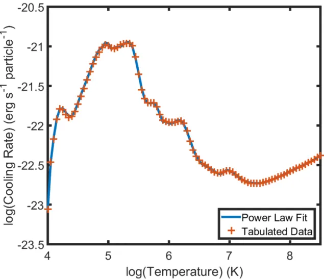
Athena handles radiative cooling by adding an external source term given by Equation 2.4 to the energy equation within the CTU integrator. As noted in Section 2.3 I use tabulated data from Sutherland & Dopita (1993) and fit piecewise power-law functions, that I calculated using MATLAB’s polyfit function, to the tabulated cooling (Figure 2.2). Between 104 and 105 K I use a 10th order polynomial. Between 105 and 106
K I use a 10th order polynomial. Between 106 and 107 K I use a 8th order polynomial. Between 107 and
108.5 K I use a 5th order polynomial. Above 108.5 K I use Equation 2.7 to calculate the emission.
SubstantialT and pressure gradients in my simulations require modification to improve the accuracy of the cooling step by sub-cycling a 2/3rd order adaptive step-size integrator (Bogacki & Shampine 1989), as follows. For each cell at each time step, ∆T is calculated using a single pass through the Bogacki-Shampine method. If the difference between the 2nd and 3rd order results exceeds 10% or if the method returns a non-physical result (i.e. ă0 K or a NaN) then ∆T for the cell is recalculated using an adaptive step subroutine. Otherwise, I keep the result from the first pass.
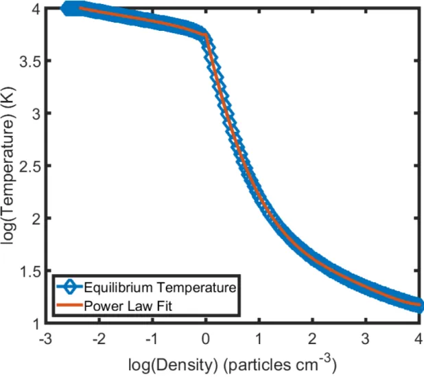
As the cooling step ends I check if the calculated ∆T deviates the cell from its radiative equilibriumT at its current density. I calculate the equilibrium temperature at different densities using root finding methods in MATLAB, then I fit the equilibrium temperature using piecewise functions with a 5th order polynomial for densities below 1.0 particles cm´3, and another 5th order polynomial for densities above 1.0 particles
cm´3 (Figure 2.3). Both fits were found using the function polyval in MATLAB. I also impose a 10 K floor
to ensure a physical result.
2.4.2 Kinetic Flux Vector Splitting
I add a backup way to calculate fluxes for the 1-5 cells (out of 6ˆN3 flux calculations) in a single
Figure 2.2: Comparison of Sutherland and Dopita tabulated cooling values and my piecewise power-law fit.
2.4.3 Integrator Modifications
Figure 2.3: Comparison of calculated equilibrium temperatures and my piecewise power-law fit.
2.5 Initial Conditions of the ISM
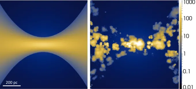
To generate a realistic initial ISM, I multiply a smooth background against a fractal density distribution to mimic embedded clouds.
2.5.1 Smooth ISM
Densities in the computational domain are a combination of halo and disk distributions given by
nhalopr, zq “nhalop0,0q ˆexp «
´Φtotpr, zq ´e 2
haloΦtotpr,0q ´ p1´e2haloqΦtotp0q c2
s,halo
ff
, (2.8)
ndiskpr, zq “ndiskp0,0q ˆexp «
´Φtotpr, zq ´e 2
diskΦtotpr,0q ´ p1´e2diskqΦtotp0q σ2
t `c2s,disk
ff
central densitynp0,0q, sound speedcs,disk“
a
kBTdisk{mHthat sets the scale height of each density profile, andedisk,halothe ratio of azimuthal to Keplerian velocity. The turbulence parameterσthelps to form a thick disk without raising its temperatures artificially (see Cooper et al. 2008).
200 pc
Figure 2.4: XZ plane slice of gas density (npr, zqin cm´3) scaled logarithmically. Left: Smooth disk before
adding fractal clouds. Right: The disk with fractal clouds.
2.5.2 Fractal Clouds
A “cloudy” ISM is mimicked by a fractal density distribution, multiplied against the smooth background disk density
npr, zq “nhalopr, zq `ndiskpr, zqNpr, zq (2.10)
withNpr, zqthe fractal density fraction of each grid cell. To make a fractal density distribution I generate a set of individual fractal clouds following Mathis et al. (2002,§2) with modifications. I repeat the Mathis et al. approach for a single fractal cloudnc times (see below), but with the constraint that first-level points must fall a distance ofěL{4 from the edge of the box. I place each cloud within the computational domain and repeat fornc fractal clouds with a scale length chosen at random between 50ăLă150 pc. Each cloud is placed semi-randomly on the computational grid to avoid excessive overlap. To set nc, I repeat until the average fractal density of the grid equals the density of a single cloud.
For models with cooling applied only when T ą 104 K, I set the disk pressure using P
diskpr, zq “
ndiskpr, zqc2s,disk. For models with cooling applied down to T ą10 K, the heating/cooling function sets the
Figure 2.5: 3D cutaway of the density (npr, zqin cm´3).
both cases whenTą3ˆ104K, cells are set to halo densities and pressures only. This prescription is given
as,
Ppr, zq “ $
’ &
’ %
nhalopr, zqc2s,halo`Pdiskpr, zq : ă3ˆ104K nhalopr, zqc2s,halo : ą3ˆ10
4K
(2.11)
I use the adiabatic exponent 5{3 and mean molecular weight 1.
Table 2.2: Parameters used for simulation setup.
Symbol Value Property
Parameters used for initial gas distribution.
nhalop0,0q 0.2 particles/cm3 Central halo density
ndiskp0,0q 100 particles/cm3 Average density in starburst
Thalo 5.0ˆ106K Halo temperature
Tdisk 1.0ˆ104K Average disk temperature
σt 60 km s´1 Turbulence parameter for disk
edisk 0.95 Rotation ratio (disk)
ehalo 0.00 Rotation ratio (halo)
Parameters used for the starburst.
Rsb 150 pc Starburst radius
Hsb 60 pc Starburst height
Parameters used for the gravitational potential.
Mss 6ˆ108M
@ Stellar spheroid mass
Mdisk 6ˆ109M@ Stellar disk mass
r0 350 pc Stellar spheroid radial scale size
a 150 pc Disk radial scale size
b 75 pc Disk scale size
zrot 500 pc Rotational scale height
Table 2.3: Grid set up for SMR models. Nx, Ny, and Nz are the number of cells in each direction. idisp, jdisp, and kdisp are the displacements measured in number of cells of that level from the base level. See the Athena documentation for more information.
Base Level First Level Second Level
Nx 64 Nx 68 Nx 128
Ny 64 Ny 68 Ny 128
Nz 64 Ny 112 Ny 160
idisp N/A idisp 30 idisp 64
jdisp N/A jdisp 30 jdisp 64
idisp N/A kdisp 16 kdisp 96
2.6 Static Mesh Refinement
Athena can employ static mesh refinement (SMR) to increase grid resolution in predesignated regions in the domain. This allows for higher resolution where needed, while decreasing the total number of processors for a single simulation, thereby enabling more extensive parameter studies. Each level of refinement doubles the resolution.
Figure 2.6: XZ plane slice of gas density (npr, zqin cm´3) scaled logarithmically. White lines indicate SMR
levels of refinement.
2.7 Starburst
I model a spheroidal central starburst using
1ą px 2
`y2 q pR2 sbq ` pz 2 q pH2 sbq , (2.12)
of radiusRsb and heightHsb. At each time step I inject mass and energy into the starburst volume at rates
9
M and E9. Each cell in the starburst region is injected with mass and energy proportional to that cell’s fraction of the total initial ISM mass within the starburst volume. At each timestep I calculate the change in the mass (dM) and energy (dE) of each cell inside the starburst using
dE dtdVcell “ 9 Enini ş
ninidVSB
(2.13)
dM dtdVcell
“
9
M nini
ş
ninidVSB
HeredVcellis the cell volume, niniis the initial density of the cell. To avoid a sharp boundary between the starburst and the ISM I apply atanhprofile tonini in the following way.
nini“npr, zq
ˆ
0.51.0´tanhpr´Rsbq
Rsb{4
˙
ˆ ˆ
0.51.0´tanhp|z| ´Hsbq
Hsb{4
˙
(2.15)
Herenpr, zqis the total density as defined by Equation 2.10.
The energy injection rate (E9) is directly related to the mechanical luminosity of the starburst by
9
E“E9SN`SW, (2.16)
withthe thermalization efficiency andL‹the mechanical luminosity (Veilleux et al. 2005). The exact value
ofdepends on the local environment of the stars in the starburst and is time dependent (Freyer et al. 2003; Veilleux et al. 2005; Strickland & Heckman 2009; Kim & Ostriker 2015). Freyer et al. (2003) show that the thermalization efficiency varies over time, ranging from 0.1 immediately after star formation to„0.01. Strickland & Heckman (2009) mention that 0.1 is the practical lower limit for the thermalization efficiency and conclude that a proper value for M82 ranges from 0.3 to just shy of 1.0. However, Kim & Ostriker (2015) find efficiency ranging from 0.1 to 1.0, but highly time dependent with rapid shifts between 1.0 and 0.1-0.3. Unless explicitly stated, for simplicity I set“1. For my models, energy is injected only as internal energy, not kinetic energy.
Like most high-resolution simulations (Suchkov et al. 1996; Cooper et al. 2008; Strickland & Heckman 2009), I combine contributions of stellar mass loss with that ablated from cold molecular clouds that are unresolved in my simulations as given in Equation 2.17.
9
M “M9SN`SW `M9cold“βM9SN`SW, (2.17)
withβ the mass loading factor. M9SN`SW is the total mass returned to the ISM from supernovae and stellar winds. It is called the central mass loading by Suchkov et al. (1996), or the mass injection rate by Cooper et al. (2008) and Strickland & Heckman (2009). I call it the mass loading rate.
Starburst99 population synthesis models (Leitherer et al. 1999) can model a starburst as either a single instantaneous starburst (SIB) or assuming continuous star formation (CSF). The energy and mass output of a SIB is dominated by stellar winds for the first 3 Myr until the first supernovae detonate. BecauseE9SN
`SW
andM9SN
and mass input from a SIB scales with starburst stellar mass as,
9
ESN`SW “7.261e40perg s´1qpMtot{107M@q (2.18)
9
MSN`SW “0.01866pM@yr´1qpMtot{107M@q (2.19)
withE9SN`SW the energy input in units of erg s´1,M9
SN`SW the mass input in units of M@yr´1, andMtot the total mass of the SIB in units of M@.
Figure 2.7: E9SN`SW (erg s´1) for SIB starbursts with initial mass ranging from 5ˆ106M@ to 1ˆ108M@.
Figure 2.8: M9SN`SW (M@yr´1) for SIB starbursts with initial mass ranging from 5
ˆ106M
@to 1ˆ108M@.
From Starburst99 population synthesis models (Leitherer et al. 1999).
For CSF, energy increases for the first 5 Myr, then remains constant thereafter due to a constant super-novae rate. Thus for my models that assume CSF, I simulate starting 5 Myr after the onset of star formation. While this is after the onset of SNs, I do not have sufficient resolution to accurately model individual SNs. Kim & Ostriker (2015) modeled individual SN inside a three phase ISM and determined that estimates of the thermalization efficiency and energy losses due to radiative cooling associated with a single SN are not accurate for grid resolutions Á 0.1 pc. Because my finest spacial resolution is 2.0 pc, I do not attempt to simulate individual SN. Future work with a more accurate sub-grid model, or greater resolution would alleviate this issue.
Figure 2.9: E9SN`SW (erg s´1) for starbursts with CSF with SFR ranging from 1 M
@yr´1to 1000 M@yr´1.
From Starburst99 population synthesis models (Leitherer et al. 1999).
the SFR (in units of M@ yr´1) by
9
ESN`SW “4.324e41perg s´1q pSFR{M@ yr´1q (2.20)
9
MSN`SW “0.1902pM@yr´1q pSFR{M@yr´1q (2.21)
2.8 Model Parameters
Figure 2.10: M9SN`SW (M@ yr´1) for starbursts with CSF with SFR ranging from 1 M
@ yr´1 to 1000
M@yr´1. From Starburst99 population synthesis models (Leitherer et al. 1999).
Models for series M assume a SIB and are divided into 1283, 2563, or 5123 fixed cells with spatial
resolution 7.8, 3.9, or 2.0 pc respectively. My low resolution models vary 0.5ďM9 ď3.5 M@ yr´1 in steps
of 0.5 M@ yr´1, and 5ˆ1040ďE9 ď1ˆ1042 erg s´1 in steps of 0.25 dex. Nine medium resolution models
range from 1.0ďM9 ď2.0 M@ yr´1 and 1ˆ1041ďE9 ď5ˆ1041 erg s´1 with another medium resolution
model atM9 “1.0 M@yr´1,E9 “1ˆ1042erg s´1. These ranges straddle the transition from blowout to no
blowout. Two high resolution models useM9 “1.5 M@yr´1,E9
“2.5ˆ1041 erg s´1 andM9
“1.0 M@yr´1,
9
E “ 1ˆ1042 erg s´1. The former was chosen to study a low energy GW, while the latter was chosen to
Table 2.4: M9 andE9 used for Fig. 3. Index refers to model number. First index in model number corresponds toM9, second toE9.
Index M9pM@yr´1q Eperg s9 ´1q
1 0.5 5.0e40
2 1.0 7.5e40
3 1.5 1.0e41
4 2.0 2.5e41
5 2.5 5.0e41
6 3.0 7.5e41
7 3.5 1.0e42
Using equation 2.18, the energy injection rates in my M series models yield a mass scale of 5ˆ106 ă M ă1ˆ108M
@. Barker et al. (2008) give a total mass for the starburst in M82 of„4ˆ107M@. Thus my
simulations exceed the range of SIBs comparable in mass to the starburst in M82 to adequately investigate the limit of a superbubble blowout.
Fujita et al. (2009) explored mass loading rates ranging from 1.7 M@yr´1to 120 M@yr´1. Strickland &
Heckman (2009) explored a much smaller range and determined a mass flow rate corresponding to M82 to be 1.4ÀM9 À3.6 M@yr´1. I choose mass loading values that are similar to Strickland & Heckman (2009).
This corresponds to values 2Àβ À15 for the most energetic starbursts and 35ÀβÀ242 for the smallest. The simulations for series M, with associated energy and mass inputs, are given in Table 2.11. Model numbers denote grid resolution, M9, E9 and cooling used. Models starting with “M1”, “M2” or “M5” cor-respond to 1283, 2563, and 5123 cells respectively. Postfix indicies designate M9 and E9 respectively, see
Table 2.4 column 1. T4 models cool to 104 K, T1 models to 10 K. To summarize my nomenclature, model
“M1 34T4” has 1283cells withM9
“1.5 M@yr´1,E9
“2.5ˆ1041erg s´1, and cooling limited toT
ą104K.
Figure 2.11: The models are arranged with increasing mass loading (in M@ yr´1) on the vertical and
increasing mechanical luminosity (in erg/s) on the horizontal. The indices on the horizontal and vertical axes correspond to the indices listed in Table 2.4 and identify the models. This arrangement is also used for Figure 4.1.
with 5123. Each model was run twice, once with cooling to 104 K then to 10 K, for a total of 122 models for series M.
Series K, S, R, and F use SMR (see§2.6) with the same configuration for all models. I use two two levels of refinement with the base grid divided into 643 cells, the first level divided into 64
ˆ64ˆ112 cells, and the second level divided into 128ˆ128ˆ160 cells. This gives spatial resolution of 15.6 pc on the base and 7.8 and 3.9 pc on each level of refinement. Thus the highest level of refinement has the same resolution as the medium resolution M series models.
The K series assumes an SIB and fixed mass loading rate either 1.5 or 3.5 M@ yr´1 and sets the energy
input to achieve a set analytic wind velocity (see§3.2, eq. 3.1). The velocity ranges from 200 to 500 km s´1in
steps of 25 km s´1, and then from 600 to 2200 km s´1in steps of 100 km s´1for a total of 60 models. Model
numbers denote first the mass loading rate, then the velocity. Thus model number K 15 1800 corresponds to mass loading rate 1.5 M@yr´1 and analytic velocity 1800 km s´1.
The S series assumes CSF and varies the SFR from 1 to 100 M@yr´1 in steps of 0.1 dex. Each model in
the S series has a fixed analytic wind velocity of 1000, 1500 or 2000 km s´1 for a total of 63 models. Model
numbers denote first the analytic wind velocity then the SFR. Thus model number S 15 79 has analytic wind velocity 1500 km s´1 and SFR 7.9 M
@yr´1.
The R series assumes CSF and varies the radius of the starburstpRSBqfrom 50 to 500 pc in steps of 0.1 dex. Each model in the R series has a fixed SFR of 10, 50 or 100 M@ yr´1for a total of 33 models. Model
numbers denote first the SFR then the starburst radius. Thus model number R 50 79 has SFR 50 M@yr´1
and starburst radius 79 pc.
The F series assumes CSF and varies the thermalization efficiency (eq. 2.16) between 0.2 and 1.0 in steps of 0.2, and varies the mass loading factor (eq. 2.17) from 1.0 to 10.0 in steps of 0.1 dex. Each model in the F series has a fixed SFR of 10 or 50 M@yr´1for a total of 110 models. Series F is similar to series M in that
I vary the mass and energy injection rates, but I set ranges of the thermalization efficiency and the mass loading factor to match the parameter space explored by Strickland & Heckman (2009) with their 2D and 1D models. Model numbers denote first the SFR, then the thermalization efficiency, then the mass loading factor. Thus model number F50 2 79 has SFR 50 M@ yr´1, thermalization efficiency 0.2, and mass loading
factor 7.9.
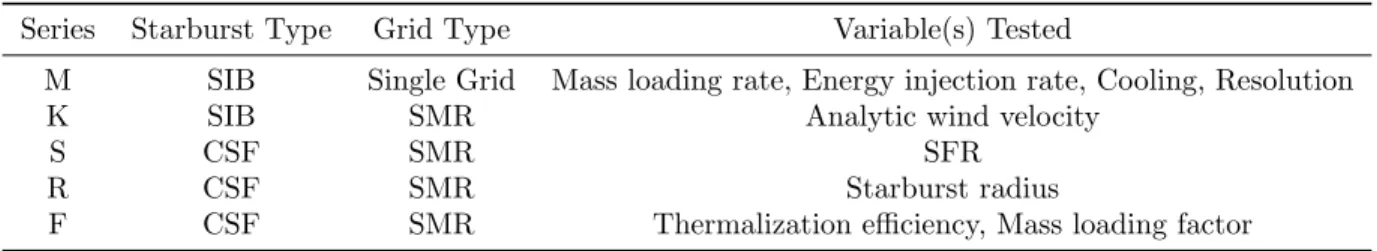
Table 2.5: Series of simulations run with basic information on each series.
Series Starburst Type Grid Type Variable(s) Tested
M SIB Single Grid Mass loading rate, Energy injection rate, Cooling, Resolution
K SIB SMR Analytic wind velocity
S CSF SMR SFR
R CSF SMR Starburst radius
F CSF SMR Thermalization efficiency, Mass loading factor
Myr after the start of the simulation will be available on my website2.
CHAPTER 3: Blowout Conditions and Structure
3.1 Wind Structure
Figures 3.1 and 3.2 show a “typical” GW in my highest resolution models (M5 34T1 and M5 27T1). They plot at 1.5 Myr a yz-slice of temperature and density together with column integrated Hαand soft X-ray emission. The mass and energy injection rates of model M5 27T1 powers a GW of terminal velocity
„1420 km s´1. My M5 34T1 model with a quarter the energy injection but 50% higher mass injection rate
still forms a GW but with terminal velocity„540 km s´1. After 1.5 Myr, model M5 34T1 has accumulated
enough energy to blow out (Fig. 3.1) but insufficient to clear the entire volume as model M5 27T1 does. Models that blow out have a hot (Á 106 K) free-wind region where the velocity is set by E9 and M9.
Embedded in the free wind are dense (ą 10 particle cm´3) filaments of warm and cold gas (
ă 5000 K) surrounding dense cores (ą100 particle cm´3) that have been swept up by the wind. These filaments are
discussed in Chapter 5. The swept-up gas substrate is shock heated toÁ107K and surrounds the free wind
as a shell.
3.2 Outflow Wind Speed
The analytic terminal wind speed of a blowout is related to E9 and M9 (see Fujita et al. 2009, based on Weaver et al. (1977) and McCray & Kafatos (1987)) as
vA”
˜ 2 ş 9 Edt ş 9 M dt ¸1{2
. (3.1)
It is related to the simulated wind speedpvwqby
vw“ξ1{2vA (3.2)
Fujita et al. (2009) give ξ “ 5{11 « 0.45 which is the fraction of E9 that drives the kinetic energy within a bubble that is embedded in a uniform ISM (Weaver et al. 1977). For comparison to analytical results, I determineξfrom my model set (Fig. 3.3). Eq. 3.2 is generally reproduced by my models: T4 models when
200 pc
Figure 3.1: A slice in the yz plane through the center of the galaxy for model M5 34T1 at 1.5 Myr. Clockwise from top left: Hαemission (log erg s´1cm´2) and temperature (log K), density (log cm´3), and soft X-ray
emission scaled as log( erg s´1 cm´2). Red box in bottom right image indicates the zoomed-in region of
Figure 5.2.
The escape velocity from the model galaxy isve«490 km s´1. ForvAăve, my simulations do not blow out. ForvA ą1.5ve, my T4 and T1 series are identical, and increased resolution does not alter the wind speed. In the transitionveăvAă1.5ve, my T4 models have higher simulated wind speeds than T1 models (Fig. 3.3 inset); both deviate from the relation in Eq. 3.2.
Using Equations 2.16 and 2.17 I can relate the analytic wind speed to the energy and mass injection rates from Starburst99 population synthesis models (Leitherer et al. 1999).
vw“
˜
2ξ ş
E9SN`SWdt
ş
βM9SN`SWdt
¸1{2
. (3.3)
200 pc
Figure 3.2: Same as Figure 4, but now for model M5 27T1 at 1.5 Myr. Red box in bottom right image indicates the zoomed-in region of Figure 5.3.
the first„3 Myr of a SIB. Because both Equations 2.18 and 2.19 depend on the total mass of the starburst, the mass cancels out and we see that the terminal wind speed depends only on the thermalization efficiency and the mass loading factor.
vw“ p2,478 km s´1q
c
2ξ
β (3.4)
Doing the same for CSF using Equations 2.20 and 2.21 gives,
vw“ p1,894 km s´1q
c
2ξ
CHAPTER 4: Emission as Blowout Tracer
When viewing starburst galaxies edge on we use emission from the superbubble to determine if a blowout has occurred. In this chapter I investigate how to use the emission from the starburst and associated superbubble to infer starburst properties. Figure 4.1 maps emission of Hαand soft X-rays for the M1 XXT1 models, viewed edge-on. Note:
1. Emission morphology reveals the threshold M9 andE9 for a blowout. As expected from Eq. 3.1, larger 9
M inhibits blow out but largerE9 promotes it.
2. Soft X-rays delineate the starburst and shell of the superbubble, and fill the free wind region (Fig. 3.1). X-rays brighten with increasingM9. For lowM9 but highE9 the starburst emits few X-rays. With higher
9
M the hot free wind has higher mass, boosting the X-ray emissivity.
To determine which emission bands can trace a blowout I define ∆ as the ratio of total emission in the lower halo (z ą85 pc) to the disk (ză85 pc). Figure 4.2 compares ∆ for different emission bands to the terminal wind speedvw. Simulations withvwą300 km s´1 have clearly experienced a blowout. Results in the blowout regime suggest the relation
∆“αvκwind. (4.1)
Hereαandκare constants. All bands follow this relation except for the cold gas (top right panel of Figure 4.2). Wind speed does not significantly affect cold gas emission, though there may be increased cold gas emission whenvwą1000 km s´1. For M series models only two simulations (M1 17 and M1 27) produced hard X-rays so I was not able to establish a relationship between wind speed and ∆. I note that the Hα
emission calculated here represents a lower bound because I do not include ionizing radiation from the stellar disk, the starburst, and other sources.
Figure 4.1: Low-resolution M1 XXT1 models at 1.5 Myr. Models are arrayed with increasing M9 (in M@
yr´1) vertical and increasing E9 (in erg s´1) horizontal. Values on axes are the same as in Table 2.4 and
correspond to indices in model numbers. Hα(red) and soft X-ray (blue) emission scaled as log(erg s´1cm´2)
4.1 How Does the Cooling Function Alter Emission?
I use three measures to determine how the different cooling limits affect the gas transported out of the galactic disk. I compare how T1 and T4 cooling affects the relation betweenvw and gas mass in the lower halo (zą85 pc), gravitationally unbound mass, and ∆.
Figure 4.2 shows that the different cooling limits do not affect ∆ for soft and mid X-rays, whereas for Hαboth ∆ andκdiffer drastically between series T4 and T1. For T4 models Hαemission in the disk is ten thousand times brighter than the lower halo, whereas for T1 models the disk is only ten times brighter. Cold gas in the lower halo (ă102 K) emits only in T1 models. Still, lower halo emission from cold gas remains 4-8 dex below that from the disk.
I sum the gas mass present in the lower halo (z ą 85 pc) over the central 500 pc. I also sum the gravitationally unbound gas mass present in the disk and lower halo over the entire computational domain. Similar to Strickland & Stevens (2000) I consider gas to be gravitationally unbound if
|vzpr, zq|`vthermpr, zq ąvescapepr, zq (4.2)
where|vzpr, zq|is the bulk velocity in each cell in the vertical direction,vthermpr, zq ”
a
3kBTpr, zq{mH and
vescapepr, zqis the escape velocity for each cell. Figure 4.3 plots unbound gas mass and gas mass in the lower halo vs. wind speed vw for both cooling limits. Forvw ą500 km s´1 there is no significant difference in the unbound mass for all temperature regimes between the T4 and T1 models. Below 500 km s´1 the T4
models still have„2ˆ105 M
@ of unbound mass. This mass is hot, thermally unbound, non-ballistic gas.
The artificially high cooling limit of the T4 models keeps the disk gas hot and thermally unbound.
Figure 4.3 reveals no difference in the total gas mass present in the lower halo between the T4 and T1 models. For all wind speeds, warm Hα emitting gas dominates in T4 models but not in T1 models. Gas mass decreases in both at highvw because the models with highest wind speed have smallM9 but large E9. Thus the wind, and by extension the lower halo, does not have as much mass.
Temperature-density plots in Figure 4.4 demonstrate differences in model series T1 and T4: three models (M2 43, M2 34, M2 25, withM9 p2.0,1.5,1.0qM@yr´1, andE9
p1.0,2.5,5.0q ˆ1041 erg s´1) of series T1 are
down the left column, and repeated for series T4 on the right. T4 models reproduce the Hα “shelf” at
„104K of Strickland & Stevens (2000) and Creasey et al. (2013). The shelf is barely evident in T1 models.
It comprises shocked gas cooling to much lower values. Reduced shelf mass explains reduced Hαgas mass in Figure 4.3.
Figure 4.2: Total emission lower halo/disk (∆) vs. simulated wind speed at 1.5 Myr for M series models. Counterclockwise from upper right: cold gas, Hα, soft X-ray, mid X-ray.
outflow as evidenced by an absence of hot gas in the lower halo. This model sits in the bottom of the intermediate regime shown in the inset in Figure 3.3.
4.2 Resolution
To examine the effect of resolution I ran my MX 34 and MX 27 models at three resolutions, and compared the wind velocities, lower halo mass, and unbound mass in the different temperature regimes. As noted in Section 2.5.2, the same initial density distribution was used for all models and was coarsened for the lower resolution models. Additionally my M5 27 and M2 27 models use the same parameters and resolutions as model numbers M01 and M04, respectively from Cooper et al. (2008).
Figure 4.3: Gas mass vs. simulated wind speed for M series models. Graphs on the left show gas gravita-tionally unbound from the galaxy. On the right, gas present in the lower halo (zą85 pc). Graphs on the top show T1 models, on the bottom T4 models. Mass measured at 1.5 Myr.
steady state wind had formed after 1.5 Myr. For all MX 34 models vw « 550 km s´1 and for all MX 27 models vw«1420 km s´1. As shown in Figure 3.3 forvwą500 km s´1 the relation given in Equation 3.2 holds irrespective of resolution. Thus the wind kinematics of a sufficiently powerful starburst are not affected by numerical resolution. But note, when vw ă500 km s´1 (see Figure 3.3 insert) wind formation depends on the resolution. Lower resolution models may experience enhanced cooling due to greater average density from unresolved features. Thus for models on the edge of a blowout, increased resolution is important for determining if a galactic wind will form.
just above the limit ofvwă500 km s´1 where resolution begins to affect the kinematics. This is evident as a slight decrease in the total unbound mass at the lowest resolution. The unbound mass of soft X-ray gas is not affected by resolution for both sets of models, but for my MX 34 models there is marked decrease in soft X-ray gas mass in the lower halo. This is due to the increased resolution of bow shocks and hot envelopes surrounding filaments, which decreases the amount of mass in that temperature regime. This effect is not seen in the MX 27 models because the superbubble has expanded to fill the entire lower halo volume. Here the mass contribution of bow shocks and hot envelopes surrounding filaments is not as significant. Related to this is an increase in unbound, warm, Hαemitting gas from ablata off of ballistic filaments. This corresponds to increased cold gas in the lower halo as higher resolution models form more well defined filaments containing cold gas.
Because there is not a significant difference in velocity and total outflow mass between my M2 and M5 models I determined that a grid resolution of 3.9 pc suffices for studying the effect of starburst and galaxy parameters on the resulting outflow. Thus for my series that employ SMR, I use a grid resolution of 3.9 pc on the highest refinement level.
4.3 Using Total Emission to Infer Starburst Properties
Figure 4.1 reveals increased X-ray emission with increasing mass loading. Using 2D and 3D models Strickland & Heckman (2009) inferred starburst properties of M82 using total X-ray emission from their models. Here I use my M and F series models to investigate the effect thatM9, E9, the mass loading factor (β see eq. 2.17), and the thermalization efficiency ( see eq. 2.16) have on the total emission from the superbubble in different temperature regimes as given in Table 2.1.
Figures 4.6 and 4.7 show total halo emission, defined as all emission from gaszą85 pc, for my M series models. The models are arrayed as in Figure 4.1 with increasing E9 horizontal, and increasing M9 in the vertical, so that each “pixel” represents a single simulation. Figure 4.6 shows total emission from cold, warm and Hαemitting gas, while Figure 4.7 shows total halo emission from hot UV, soft, mid, and hard X-ray emitting gas.
increasingβ (ranging from 1.0-10.0) are vertical.
With a SFR of 10 M@yr´1, theE9 andM9 of my F10 series correspond roughly to the M series simulations
in the two right most columns of Figure 4.1, the highest energy models, but with a larger total mass loading range. The absence of X-ray halo emission for models with highM9 and lowE9 indicates that the outflow from the starburst has been quenched. Despite the absence of an outflow, the quenched models still have trace amounts of cold, warm and Hαemitting gas, while quenched models do not produce X-ray emission. Only three of my F series models had their outflows quenched, compared to 19 of my M series. In the quenched models cooling dominates to prevent a wind from forming.
In Figure 4.10 I compare soft and mid X-ray halo emission for my F10 XX XX models with a SFR of 10 M@yr´1, and my F50 XX XX models with a SFR of 50 M@ yr´1. The F50 models have higher total halo
emission, but as can be seen in the soft X-ray panels the same models are quenched regardless of SFR. A starburst with a higher SFR inputs more energy and this can be seen by comparing the mid X-ray emission. More models have mid X-ray halo emission.
Inside each panel of Figures 4.6, 4.7, 4.8, and 4.9 wind velocity increases from top left to bottom right, with the simulation situated in the bottom right corner having highest velocity. While the total halo emission from all bands generally increases with higher velocity winds, the models with the highest velocity outflows do not always have the highest total emission. This is evident for hot UV and soft X-ray emission from my M series, and is even more evident in all bands for my F series, with the exception of mid and hard X-rays. In all of these models, higher velocity is achieved by increasingE9 relative toM9, which increases the fraction of the gas at higher temperature. As gas is pushed to higher temperatures, total Hα, UV and soft X-ray emission is decreased, while mid and hard X-ray emission increases.
For both my M and F series, the greatest Hα, hot UV and soft X-ray emission comes from models with wind velocity „ 1500 km s´1. Above this, the total halo emission and ∆ decrease, indicating that the
relationship between total emission and wind velocity given in Equation 4.1 only holds for Hα, hot UV and soft X-ray emission when wind velocitiesă1,500 km s´1. Above that point mid or hard X-ray emission can
Figure 4.7: Total halo emission from M series models arrayed in same configuration as Figure 4.1 with increasingE9 horizontal, and increasingM9 in the vertical. Clockwise from top left total emission in erg s´1
for hot UV, soft X-ray, hard X-ray, mid X-ray gas. While the color bar assigned to each emission band has a lower limit, the actual emission from models at the lower limit is 0 erg s´1. The lower limit has been set
Figure 4.8: Total halo emission from F series models arrayed with increasing thermalization efficiency () horizontal, and increasing mass loading factor (β) in the vertical. Clockwise from top left total emission in erg s´1 for cold, warm low, Hα, warm high gas. While the color bar assigned to each emission band has a
lower limit, the actual emission from models at the lower limit is 0 erg s´1with the exception of warm high
Figure 4.9: Total halo emission from F series models arrayed with increasing thermalization efficiency () horizontal, and increasing mass loading factor (β) in the vertical. Clockwise from top left total emission in erg s´1 for hot UV, soft X-ray, hard X-ray, mid X-ray gas. While the color bar assigned to each emission
band has a lower limit, the actual emission from models at the lower limit is 0 erg s´1with the exception of
Figure 4.10: Panels on the right are soft and mid X-ray emission from Figure 4.9 from models F10 XX XX with a SFR of 10 M@yr´1. Panels on the left are from soft and mid X-ray emission from models F50 XX XX
CHAPTER 5: Embedded Filaments
5.1 Expanding Bubbles
Many GWs contain long optical and X-ray emitting filaments (Bland & Tully 1988; Veilleux et al. 1994; Shopbell & Bland-Hawthorn 1998; Devine & Bally 1999; Strickland et al. 1997, 2002). In my simulations, filaments appear by a combination of three processes.
1. Limb brightening from the shocked edge of the superbubble (Cecil et al. 2002).
2. Disruption of a cool dense cloud by the supersonic wind (Cecil et al. 2002; Cooper et al. 2009). 3. Merging bubbles that rise from the starburst region (Joung & Mac Low 2006; Melioli et al. 2013).
Limb brightened filaments appear in Figures 4.1 and 3.2 at the edge of the shocked region; they are broad (100´200 pc) without well defined boundaries. They have no significant vertical motion because they represent the edge of the wind region. Embedded in these regions may be smaller filaments formed through processes 2 and 3 as discussed below.
Cold dense clouds are overrun by the supersonic hot wind, which exerts a ram pressure on the cloud, disrupting it, stripping off material and elongating it into a filament. Examples of disrupted clouds can be seen in the density plots in Figures 3.1 and 3.2. While these disrupted clouds are present in my simulations, to fully resolve them would require resolutionă0.1 pc (see Cooper et al. (2009)) compared to my maximum of 2 pc.
Due to inhomogeneities in the starburst, multiple bubbles form that sweep up and squeeze the ISM. With continued expansion, the shells merge to coalesce the gas into thin (ă 50 pc) filaments. In my models, many of these filaments emit little Hαbefore dispersing within a Myr by shock heating and ablation, or disrupting by Kelvin-Helmholtz instabilities.
Z
Figure 5.1: Cartoon of two merging superbubbles viewed side-on, combining filament formation scenarios 2 and 3. Their contact forms a filament from ISM swept up and compressed by the wind. To persist, this filament must be anchored to a mass loading source to continuously replenish its shocked, dense gas.
Figures 5.2 and 5.3 compare models M5 34T1 and M5 27T1 respectively to show examples of filaments forming through a combination of cloud disruption and merging bubbles. These filaments are embedded in a GW of 400 ăv ă 2000 km s´1. The densest material has a velocity of
À 50 km s´1 whereas ablated
material 200ăvă500 km s´1. Thus the dense cores of the filaments are hardly moving with respect to the
disk. The wind flows by, ablating and collimating the filaments. The velocity gradient of its ablata resembles the homologousvprq9rvelocity gradient mapped in NGC 3079, although velocities are lower than the 1500 km s´1 observed (Cecil et al. 2001, 2002).
5.2 Mass Anchors
Model M5 34T (Fig. 5.2) has sufficient energy to form a GW, but the wind does not disrupt all filaments. As shown in Figure 5.2, two distinct bubbles emerge from the central starburst. Their boundaries merge to form a dense filament that stretchesą100 pc back to anchor on the starburst reservoir. The 540 km s´1wind
ablates mass off the reservoir, and pushes it into the filament that by 1.5 Myr has extendedą400 pc above the disk plane to drift along at only 50´100 km s´1. Due to continual mass loading at its base, the
filament stays anchored allowing it to persist and grow. At some point the filament should disrupt entirely due to either Kelvin-Helmholtz instabilities or heating and evaporation. But my resolution is insufficient to maximize filament survival time (see Cooper et al. 2009).
5.3 Filament Lift Off
In model M5 27T1 (Fig. 5.3) the filament again forms along the bubble contact. But now, after 1 Myr it detaches from the disk reservoir and lofts into the free-flowing wind of the now merged bubbles. This filament differs from its slow counterpart model M5 34T1; it has a larger cross section to the impinging wind, so it fragments more due to Kelvin-Helmholtz instabilities. The surrounding wind flows at 1420 km s´1while the
filament moves at 0´50 km s´1 before lift off but attains 200
´500 km s´1thereafter. This filament would
0.5 Myr
0.625 Myr
100 pc
0.75 Myr
1.0 Myr
1.25 Myr
0.5 Myr
0.625 Myr
100 pc
0.75 Myr
1.0 Myr
1.25 Myr
CHAPTER 6: Synthetic Absorption Lines
In Chapter 4 I showed how total halo emission can be used to infer galactic wind velocity and starburst properties for edge on galaxies. For face on galaxies, absorption lines can probe kinematic properties of the three phase medium of the galactic wind. To probe cold, warm, and hot gas phases I synthesize absorption lines of various ions. Typically only the warm phase has been probed using absorption lines (Heckman et al. 2000; Martin 2005; Rubin et al. 2014; Chisholm et al. 2015, 2016), but more recent work (Ho et al. 2016, e.g.) and future surveys using ALMA and the Square Kilometer Array will focus on absorption from colder, molecular and atomic gas. All surveys cited above have noted the presence of asymmetric absorption profiles from warm and cold gas entrained in the galactic wind.
To help the interpretation of absorption profiles, I first use a simple formulation in Section 6.1 to generate asymmetric profiles seen in observations, then in Section 6.2 I give a more general formulation to generate absorption lines of specific ions, and finally in Section 6.3 I study relationships between SFR, SFR density (ΣSFR) and the analytic wind velocity.
6.1 Simple Absorption Profiles
For my simple formulation I synthesize absorption lines for three temperature regimes, denoted “molecu-lar”, “warm”, and “soft X-ray”, that correspond to the cold, Hαand soft X-ray temperature ranges in Table 2.1. A trivial, optically thin line source function suffices for kinematical signatures of the three temperature regimes. Absorption spectra are derived by integrating optical depth in N cells along the column viewed perpendicular to the disk
τpvchq “ N
ÿ
i
τipvchq. (6.1)
The velocity channels have a resolution of 10 km s´1 and range from -1800 km s´1to 200 km s´1.
the asymmetry would require running additional models to study how the number of filaments affects line asymmetry. My K series used initial conditions that produced more filaments than my M series and as seen in Figure 6.5 the absorption line from hot gas does not have as much asymmetry. This would indicate that the asymmetry of absorption lines in hot gas depends more on the number of filaments in the wind. Model M5 34T1 shows two spikes in this absorption profile. The faster spike corresponds to the free wind inside the expanding bubble, the slower to absorption in the bubble shell. This shell has left the computational grid in model M5 27T1.
The “warm” line traces filaments and clouds caught in the gas but moving much slower, so maximum extinction is at much lower velocity. The long tail of this profile traces ablata accelerating off the filaments. The “molecular” line shows a similar tail, although that absorption is more varied because multiple clouds contribute. In both the “warm” and “molecular” profiles shown in Figure 6.1 there is absorption at positive velocities. These features result from clouds initially at the edge of the lower halo, but not directly above the starburst. They were perturbed by the shock from the starburst but not blown out by it and have begun to fall towards the disk. For absorption from an arbitrary ion found in the neutral medium, I would expect an acceleration tail similar to that in the warm and molecular lines.
The asymmetric “warm” and “molecular” absorption line profiles are similar to observed SiII, SiIII, OI,
CII (see Wofford et al. 2013, Fig. 11, especially KISSR 242 and KISSR 1578), and Lyα (see Jones et al.
2012, Figs. 5 and 6) profiles in starburst galaxies. The shape also matches analytical predictions (Scarlata & Panagia 2015).
6.2 Full Absorption Profiles
I now calculate absorption profiles for specific ions to probe the kinematics of the three phase medium in the galactic wind.
The absorption coefficient for a single velocity channel (vch) is,
κpvchq “Npvchqapvchq (6.2)
where Npvchq is the column density and apvchqis the absorption per atom. Assuming contributions from Doppler broadening and spontaneous radiative transitionsapvchqis given as,
apvchq “
πe2 mec
1
? π
1 ∆ν1{2
f Hpvchq. (6.3)
the Gaussian component,f is the oscillator strength, and Hpvchqis a Voigt profile. The Gaussian HWHM is calculated using Equation 5.70 from Kwok (2007),
∆ν1{2“
2
c c
2kBT
m lnp2qν0 (6.4)
withkB Boltzmann’s constant,T the gas temperature,mthe atomic mass of the ion, and ν0 the frequency
of the line center from the NIST Atomic Spectra database (Kramida et al. 2015). I calculate the Voigt profile (Hpvchq) using Matlab code1 written by Dr. Nikolay Cherkasov that employs the method of Schreier (2011). The method uses the complex error function to quickly generate an approximate Voigt profile using the HWHM of the Gaussian and Lorentzian components. The Lorentzian HWHM comes from the sum of all possible Einstein coefficients (Einstein 1905) that gives the transition strength for each quantum level (Kwok 2007, see eq. 5.59). Transition and oscillator strengths of each line are in the NIST Atomic Spectra database. An example of a Voigt profile is shown in Figure 6.2.
Figure 6.2: Example of a Voigt profile for the 1190 ˚A Si II line at 20,000 K.
on the cell density and the ionization fraction (Mazzotta et al. 1998). Examples of the computed ionization fractions for Si I-XIII are shown in Figure 6.3. I then use the absorption coefficient for each cell for each to calculate the optical depth using,
τipvchq “κipvchqdz. (6.5)
The optical depth is then summed along the line of sight. The absorption profile for a given ion along a line of sight is,
Ipvchq “I0pvchqe´τpvchq (6.6)
The resulting profile is then averaged over all lines of sight directly over the starburst and then re-normalized. Figure 6.4 gives an example of a synthetic absorption profile for the O I 1302.17 ˚A line. I use a channel resolution of ∆vch“0.25 km s´1.
Figure 6.3: Ionization fractions for Silicon ions (Mazzotta et al. 1998).
Following the method of Chisholm et al. (2015) I calculate thevcen andv90velocities from the line. The vcen velocity at half of the FWHM, and v90 is the velocity where the absorption profile returns to 90% of
full intensity. Thusvcen measures the bulk velocity of the absorbing gas for a particular temperature range
and gas phase, andv90measures the maximum velocity of the gas phase and temperature range. I use these
Figure 6.4: Synthetic absorption profile for the O I 1302.17 ˚A line. S 20 100 model with an analytic wind velocity of 2,000 km s´1and a SFR of 10 M
@yr´1. Vertical lines indicatevcen andv90 velocities.
6.3 Relationships from Absorption Profiles
In this section I use my K, S, and R series to investigate the relationships betweenvcenandv90velocities,
and the analytic wind velocity (vA from Equation 3.1), the SFR, and the SFR density (ΣSFR), along with
the outflow velocities of the multi-phase medium.
In Figure 6.5 I plot synthetic absorption lines for Si I, II, VII, and XIII. These four lines probe gas temperature ranges corresponding toă1e4 K, 1e4´2.5e4 K, 4.5e5´7e5 K, and 2e6´1e7 K respectively. The gas producing the Si I and II absorption lines is moving „ 300 km s´1 slower than the hotter gas
producing Si VII and XIII absorption. In Chapter 5 I noted that the dense gas inside the filaments is moving much slower than the hot, diffuse gas. That same difference in velocity is observed here in my synthetic Si lines. The difference between the Si I and XIII lines is even greater if we consider the v90 velocities, a
difference of„700 km s´1.
The Si VII and XIII lines are also asymmetric but smooth. The smooth shape indicates that the hot gas transitions seamlessly through different velocities as it accelerates from the galaxy. Because the hot gas fills the inside of the superbubble, it is not fragmented and clumpy unlike the cold gas. The asymmetries are still present due to the hot gas being accelerated as it moves off of the plane of the galaxy.
Figure 6.5: Synthetic absorption lines for Si I, II, VII, and XIII from my K 15 1800 model, which has avA of 1800 km s´1.
To understand how the velocity of the gas changes with increasing temperature, I plot in Figures 6.6 and 6.7 the vcen and v90 velocities respectively for Si I-XIII from my S series models. The plots include data
from models withvA of 1000, 1500, and 2000 km s´1 at SFR of 10, 50, and 100 M@ yr´1.
In Figure 6.6 we see three distinct velocity regimes corresponding to Si I-II, Si III-XI, and Si XII-XIII. These correspond to temperatures ă2.5e4 K, 2.5e4´2e6 K, and ą2e6 K, respectively. As is noted by Equation 3.5, the wind velocity does not depend on the SFR. For models withvA“1000, 1500 km s´1there is no significant difference in vcen, except for the model with SFR 10 M@ yr´1 andvA“1500 km s´1. In this case thevcen for the midrange ions is„200 km s´1lower than the models with SFR 50 or 100 M@yr´1.
For models withvA “2000 km s´1 there is a difference invcen for all ions and for all SFR with increasing
velocity for increased SFR.
In Figure 6.7 I show the v90 velocities for the same models as in Figure 6.6. A similar trend is evident
with the three distinct velocity regimes, though less obvious for models with vA “ 1000. The velocities for different SFR are similar, indicating that the maximum velocity for a giving ion depends on the wind velocity not the SFR. The only exception is for low SFR where cooling may dominate.
Figure 6.6: Thevcenvelocity of all Si ions for select S series models. Blue lines are for models withvA“1,000 km s´1, green for v
A“1,500, and red forvA“2,000. Solid lines with ’x’ indicate models with SFR of 10 M@ yr´1, dashed lines with circles indicate a SFR of 50 M@ yr´1, and dot dashed lines with pentagrams
indicate models with SFR of 100 M@ yr´1.
Figure 6.7: Thev90velocity of all Si ions for select S series models. Blue lines are for models withvA“1,000 km s´1, green for v
A“1,500, and red forvA“2,000. Solid lines with ’x’ indicate models with SFR of 10 M@ yr´1, dashed lines with circles indicate a SFR of 50 M@ yr´1, and dot dashed lines with pentagrams
indicate models with SFR of 100 M@ yr´1.
velocity of the warm gas is affected by differentvAand SFRs. For a givenvA, thev90velocity increases with
increasing SFR untilÀ0.8vA. But according to Equation 3.5 the outflow velocity should not depend on the SFR.
To resolve this dilemma in Figure 6.9 I plot thev90velocity of Si XIII for my S series models. This shows