Index Catalog // Carolina Digital Repository

(1)

A Multisensor Evaluation of the Asymmetric

Convective Model, Version 2 in Eastern Texas

by

Jenna Sue Kolling

A thesis submitted to the faculty of the University of North Carolina at Chapel Hill in partial fulfillment of the requirements for the degree of Master of Science in the

Environmental Sciences and Engineering.

Chapel Hill 2011

Approved by:

William Vizuete, Advisor

Harvey Jeffries, Reader

(2)

c

! 2011

(3)

ABSTRACT

JENNA SUE KOLLING: A Multisensor Evaluation of the Asymmetric Convective Model, Version 2 in Eastern Texas.

(Under the direction of William Vizuete.)

Although there have been a variety of planetary boundary layer (PBL) schemes

developed to represent the effects of turbulence in daytime convective conditions,

un-certainties correlated with these schemes remain a large source of inaccuracy in

me-teorology and air quality model simulations. This study evaluates a new combined

local and nonlocal closure PBL scheme, the Asymmetric Convective Model, version 2

(ACM2) in eastern Texas against PBL observations taken from ten radar wind profilers,

a ground-based lidar, and multiple daytime radiosonde balloon launches. Comparisons

are made between these observations and outputs from the Weather Research and

Forecasting (WRF) model version 3.1 with the ACM2 PBL scheme option, as well as

outputs from the meteorological modeling that is currently being used to develop ozone

control strategies in the HGB area. Results show that the WRF-ACM2 combination is

much more accurate at representing the spatial and temporal evolution of the PBL in

Eastern Texas.

(4)

List of Tables

3.1 RWP station divisions according to geographic location . . . 10

(6)

List of Figures

2.1 Map of Eastern Texas showing radar wind profiler locations . . . 7

2.2 Map of downtown Houston, TX and UH-Moody Tower . . . 8

3.1 Root mean square error for all radar wind profiler stations . . . 11

3.2 Time series plots of median hourly PBL heights . . . 13

3.3 Time series plots of median 2-meter temperature and 2-meter mixing ratio 15 3.4 Time series plots of median sensible and latent heat fluxes . . . 16

3.5 Lidar backscatter image from Moody Tower, TX on September 7, 2006 18 3.6 Time series of modeled and observed PBL heights on September 7, 2006 at Moody Tower, TX . . . 19

3.7 Vertical profiles of potential temperature and mixing ratio from

(7)

Chapter 1 Introduction

Among the most important meteorological parameters that influence air quality is

the volume of well-mixed air below the free troposphere called the planetary boundary

layer (PBL). The PBL interacts directly with the Earth’s surface on a time scale of

hours, and with a height that is variable in space and time, ranging between hundreds of

meters to several kilometers. During the daytime, solar heating of the Earth’s surface

can generate buoyant turbulent eddies that efficiently mix the air within the PBL.

Consequently, particulate matter and gases are diluted at the ground level while a

rapidly growing PBL entrains aged pollutants from the free troposphere above. Our

ability to accurately predict air quality is limited by a lack of knowledge of the physical

influences on PBL structure, making it particularly difficult to model the early morning

rise and afternoon decay. These physical influences include turbulence intermittency,

horizontal heterogeneity, and rapid time changes (Dabberdt et al., 2004).

An accurate depiction of the diurnal evolution and vertical mixing within the PBL

is necessary for realistic air quality simulations (Seaman, 2000; Ku et al., 2001; Zhang

et al., 2007). Largely driven by surface heating, the development of the PBL in

mesoscale meteorological models relies on realistic simulations of surface fluxes of

mois-ture and heat. Land surface models (LSMs) are used to parameterize these physical

(8)

vertical transport of heat, moisture, momentum, and trace chemical mixing ratios.

Although a variety of PBL schemes have been developed to represent the effects of

turbulence in convective conditions, uncertainties correlated with these schemes

re-main a large source of inaccuracy in model simulations. Most existing PBL schemes,

namely local and nonlocal closure models, do not consider both small- and large-scale

turbulence. In local closure PBL schemes, turbulent fluxes are computed as functions

of local gradients, confining vertical mixing to adjacent grid cells. As a result, local

closure schemes, including the Mellor-Yamada-Janjic (Janjic, 1990, 1994) cannot

realis-tically simulate convective conditions, which are characterized by large eddies that can

sometimes have a size similar to the boundary layer height itself (Brown, 1996).

Sim-ple nonlocal closure models, such as Blackadar (1978) and the Asymmetric Convective

Model, version 1, (ACM; Pleim and Chang, 1992) represent only large-scale transport

driven by convective plumes, neglecting small-scale turbulent mixing. Although the

use of non-local methods in models attempting to simulate the PBL has increased, a

method that can accurately represent the diurnal PBL must combine both local and

nonlocal components of vertical transport.

The recently developed Asymmetric Convective Model Version 2 (ACM2) PBL

scheme (Pleim, 2007a) includes an eddy diffusion component in addition to the explicit

nonlocal transport of the original ACM. Preliminary testing with controlled, offline

experiments showed that ACM2 was able to simulate realistic PBL heights,

tempera-ture profiles, and surface heat fluxes. Spatially and temporally limited observational

datasets allowed for a preliminary evaluation of ACM2 in the fifth-generation

Penn-sylvania State University-National Center for Atmospheric Research Mesoscale Model

(MM5) (Pleim, 2007b). When compared to two radar wind profilers (RWP) located in

Pittsburgh, PA, and Concord, NH, the model tended to simulate the morning rise in

(9)

morning warm bias in MM5 rather than a limitation of ACM2. Comparisons were also

made against vertical profile measurements taken from radiosondes launched twice a

day in Minneapolis, MN and Little Rock, AS. Data from these profiles showed very

close comparisons between observed and modeled potential temperature and relative

humidity (Pleim, 2007b). Although initial testing of the ACM2 scheme showed good

agreement with this limited dataset of observations, a more spatially and temporally

diverse set of observations is necessary to further evaluate ACM2 for use in regulatory

air quality models.

Southeast Texas, especially the Houston Galveston Brazoria (HGB) eight-hour

ozone (O3) nonattainment area, offers a unique dataset to address some of the open

questions remaining in the preliminary analysis. Since the HGB area is in

nonattain-ment of the National Ambient Air Quality Standard (NAAQS) forO3, considerable

re-sources have been spent on surface and aloft measurements. A variety of instrumented

observations were taken during The Second Texas Air Quality Campaign (TexAQS II)

(Parrish et al., 2009), which lasted from January 2005 to December 2006, and had

an intensive period of operations between August and October 2006, including the

TexAQS II Radical Measurement Project (TRAMP) (Lefer and Rappengl¨uck, 2010).

These measurements from both the TexAQS II and TRAMP field studies allow for an

extensive view of the horizontally and vertically heterogeneous PBL in Eastern Texas

and downtown Houston, and provide a rare opportunity to evaluate the new ACM2

PBL scheme.

The HGB area, which is subject to frequent highO3episodes due to the interactions

between complex coastal meteorology, emissions of ozone precursors, and atmospheric

chemistry, is a severe test for a meteorological model. Land and sea breeze circulations

and how they interact with larger-scale synoptic systems, such as the typical

summer-time high pressure over the Gulf of Mexico, have been found to play a crucial role in

(10)

the formation ofO3 in Houston (Banta et al., 2005; Darby, 2005; Vizuete et al., 2008).

Consequently, Houston’s complex meteorology presents a unique challenge for modeling

the spatially and temporally diverse PBL height, a critical component for

understand-ing the formation of ozone and other pollutants (P´erez et al., 2006). As a result of this

complexity, considerable resources have been spent on the development of

meteorologi-cal and air quality modeling episodes in support of a State Implementation Plan (SIP)

for attaining the NAAQS for O3. The retrospective modeling used for the current SIP,

prepared by the Texas Commission on Environmental Quality (TCEQ, 2010), includes

the August-October 2006 TexAQS II period. The availability of this TCEQ

meteoro-logical modeling presents a ready comparison for our evaluation of ACM2 against an

existing regulatory modeling episode.

The objective of this study is to evaluate the ACM2 PBL scheme for use in

reg-ulatory air quality models by leveraging the advanced observational data available in

the HGB area. Specifically, we will be evaluating the ACM2 PBL scheme’s ability to

accurately simulate the morning growth, maximum height, and evening collapse of the

PBL while predicting realistic profiles of temperature and humidity. These results will

then be compared with those predicted by the meteorological model currently being

(11)

Chapter 2 Methodology

2.1 Model Configuration

This study compares two models used to simulate the meteorology of Eastern Texas

between August and October of 2006. One developed by the Environmental Protection

Agency for research purposes (EPA-WRF), the other developed by TCEQ for

regula-tory purposes (TCEQ-MM5). The EPA used the Weather Research and Forecasting

(WRF) model version 3.1 (Skamarock et al., 2008) with the ACM2 PBL scheme

op-tion (Pleim, 2007a,b). The TCEQ simulaop-tion uses the Fifth Generaop-tion Meteorological

Model (MM5, version 3.7.3) developed jointly by the National Center for Atmospheric

Research and Pennsylvania State University (Grell et al., 1994) with the Eta PBL

scheme option, which is the Mellor-Yamada scheme as used in the Eta model (Janjic,

1990, 1994). The Eta PBL scheme is a local closure model, determining vertical mixing

from predicted turbulent kinetic energy.

In addition to the ACM2 PBL Scheme, EPA-WRF physics options included the

Pleim-Xiu land-surface model (PX LSM; Xiu and Pleim, 2001) with the Pleim

sur-face layer scheme (Pleim, 2006), the rapid radiative transfer model for shortwave and

longwave radiation (Mlawer et al., 1997), the Kain-Fritsch 2 cumulus parameterization

(12)

Gettelman, 2008).

The TCEQ-MM5 physics options include the NOAH land-surface model (Ek et al.,

2003), the rapid radiative transfer model, Grell cumulus parameterization, and the

simple ice microphysics. In MM5, observed parameters were assimilated during the

model run through a process called four-dimensional data assimilation (FDDA). The

fine scale 4-km domain was nudged to observational data obtained from radar wind

profilers during TexAQS II. To improve the representation of wind fields and other

parameters in MM5, the land use characteristics and sea surface temperatures on all

domains were updated with high-resolution satellite measurements. Details of the

ob-servational nudging are given in Appendix A of the TCEQ report of the Protocol for

Eight-Hour Ozone Modeling of the Houston Galveston/Brazoria Area (TCEQ, 2010).

The Meteorology-Chemistry Interface Processor (MCIP; Byun et al., 1999) version

3.5 was used to process the WRF and MM5 outputs by performing horizontal and

vertical coordinate transformations and defining gridding parameters (Otte and Pleim,

2010). The MCIP outputs for both models resulted in a 4-km gridded domain centered

over Eastern Texas. The episode period is August 13-October 10, 2006, excluding

August 23-26 and September 30 due to missing MM5 modeling data.

2.2 Observations

Observational datasets used in this study came from TexAQS II, a major field study

conducted in eastern Texas between June 2005 and October 2006, with an emphasis

on the Houston O3 non-attainment region. Meteorological parameters important to

air quality were collected via radar wind profilers (RWPs, Knoderer and MacDonald,

2007), radiosondes (Rappengl¨uck et al., 2008), and a ground-based lidar (Flynn, 2006).

(13)

was in operation during the entire month of September and multiple radiosondes were

launched per day only during high ozone events in September 2006.

2.2.1 Radar Wind Profilers

A vital component of the TexAQS II field study was a network of ten 915-MHz RWPs.

As shown in Figure 2.1, the RWPs were scattered throughout Eastern Texas, placed at

varying elevations and distances from the coast. After undergoing a rigorous quality

control procedure using the Webber-Wuertz algorithm and manual inspection,

reflec-tivity (signal-to-noise ratio) data from the RWPs were used to estimate hourly heights

of the daytime convective boundary layer, with occasional missing reports (Knoderer

and MacDonald, 2007). The off-shore Brazos site was not used for this study due to a

significant amount of missing data.

Figure 2.1: Radar wind profiler locations (blue squares) and major cities (red circles) in Eastern Texas during the TexAQS II field campaign. Color shading shows terrain elevation (Wilczak et al., 2009).

(14)

2.2.2 Radiosondes

Radiosonde balloons obtain profiles of temperature, pressure, and relative humidity

as they ascend through the atmosphere. Normally they are launched twice a day, but for

ten days with highO3forecasts during September of 2006, five additional balloons were

launched from the University of Houston (UH) Moody Tower (Figure 2.2) in downtown

Houston, TX. In addition to the radiosonde outputs, vertical profiles were inspected

and PBL heights were provided for each balloon launch (Rappengl¨uck et al., 2008).

Figure 2.2: Location of the UH-Moody Tower measurement site (Lefer and

Rap-pengl¨uck, 2010).

2.2.3 Lidar

A ground-based scanning micropulse lidar was deployed on the roof of the UH-Moody

Tower (Figure 2.2) during September of 2006 for vertical profiling of the atmosphere.

The PBL typically has higher concentrations of aerosols compared to the free

tropo-sphere, which means lidar backscatter profiles exhibit a significant negative gradient

at the PBL top. Lidar backscatter profiles were visually analyzed to determine PBL

(15)

Chapter 3 Results

For this study, observational data was derived from radar wind profilers, a

ground-based lidar, and radiosonde balloon launches. This observational data was used to

evaluate meteorological parameters of importance to air quality for direct comparison

to outputs from two meteorological models. These include direct comparisons of the

WRF model version 3.1 with the ACM2 PBL scheme option, and MM5 version 3.7.3

with the Eta PBL scheme option, which is the meteorological modeling used for the

HGB eight-hour O3 standard SIP.

Figure 3.1(a-c) shows the root mean square error (RMSE) between the hourly

day-time MM5 and WRF predicted PBL heights and the hourly dayday-time RWP derived

PBL heights for all RWP site locations. Equation 3.1 shows an example of the RMSE

calculation for the WRF model at time t.

RMSEWRF =

!

Et((PBLWRF,t−PBLRWP,t)

2

) (3.1)

where Et represents the error at time t, PBLWRF,t represents the WRF calculated PBL

height at timet, and PBLRWP,t represents the RWP derived PBL height at time t.

RWP locations in Figure 3.1(a-c) are ordered along the x-axis according to location,

(16)

to the coast. Figure 3.1a shows the average RMSE of each model between the hours of

8am-11am, representing the models’ error in predicting the morning rise of the PBL.

MM5 had a larger average RMSE than WRF at all 10 stations, ranging from 20m larger

at Longview to 130m larger at Beaumont. Although WRF predicted more realistic PBL

heights on average than MM5 during the morning hours, there is a notable increase of

about 100m in the WRF RMSE at locations nearer to the coast. Figure 3.1b shows

the average RMSE of both models at predicting the daily peak PBL (note the y-scale

increase). MM5 had a much larger error than WRF at all 10 stations, ranging from

90m larger at Arcola to 410m at Cleburne, where MM5 had more than double the

average RMSE of WRF (735m vs. 325m, respectively). Figure 3.1c shows the RMSE

between the hours of 4pm-7pm, representing the models’ error in predicting the evening

collapse of the PBL. Again, MM5 had a much larger error than WRF, ranging from

130m higher at Beeville to 800m higher at Cleburne.

To further investigate the meteorological models’ ability to accurately predict the

morning rise, afternoon peak, and evening collapse of the PBL, we looked at the

ob-served temporal evolution of the PBL from the RWPs. The ten RWP stations were

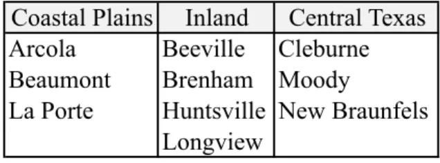
divided into three categories according to their location, displayed in Table 3.1.

Table 3.1: Ten RWP stations divided into three categories based on geographic location.

Coastal Plains Inland Central Texas Arcola Beeville Cleburne Beaumont Brenham Moody

La Porte Huntsville New Braunfels Longview

Figure 3.2(a-c) displays the modeled and observed median PBL for these three

regions. The Central Texas location (Figure 3.2a), with drier land use and precipitation

(17)

!!! ! !!!!!!!!!!!!!!!!!!!!!!!!!!Inland <---> Coast

! !! !!! ! ! ! 0 100 200 300 400 500 600 Cleburne Moody New Braunfels

Longview Huntsville Brenham Beeville ArcolaBeaumont La Porte

RMSE (m)

Morning Rise (8am ! 11am)

MM5 WRF 0 100 200 300 400 500 600 700 800 900 Cleburne Moody New Braunfels

RMSE (m) Daily Peak MM5 WRF 0 200 400 600 800 1000 1200 1400 Cleburne Moody New Braunfels

RMSE (m)

Evening Collapse (4pm ! 7pm)

MM5 WRF

(a)

(c) (b)

Figure 3.1: Root mean square error for each RWP station location (Ordered furthest inland on the left to nearest to the coast on the right) for the (a) morning rise PBL height (8am-11am), (b) afternoon peak PBL height, and (c) evening collapse PBL height (4pm-7pm).

(18)

of over 2000m, which is consistent with the findings of Wilczak et al. (2009) and Hu

et al. (2010). Figure 3.2a shows that the MM5 model is severely under-predicting the

median height of the PBL in the late morning and afternoon for the Central Texas

region by as much as 870m at 1600 CST. The WRF model is more accurate for this

time period, with the largest over-prediction of 155m occurring at 1100 CST. Both

the WRF and MM5 models predicted an earlier PBL collapse at the Central Texas

locations when compared to observations, with MM5 under-predicting by as much as

1350m at 1800 CST, while WRF under-predicted by 275m at the same time. A similar

pattern was found at the Inland and Coastal Plains locations (Figures 3.2-b,c), with

WRF slightly over-predicting the height of the afternoon median PBL by 260m at 1600

CST in Figure 3.2b, and 240m at 1300 and 1500 CST in Figure 3.2c. MM5

under-predicted the afternoon median PBL height by as much as 700m at 1400 CST at the

Inland locations (Figure 3.2b) and 540m at the Coastal Plains locations (Figure 3.2c).

At the Inland locations, MM5 collapsed the PBL too early, severely under-predicting

the PBL by 865m at 1800 CST (Figure 3.2b), while WRF closely followed the observed

PBL collapse with an under-prediction of only 110m at 1800 CST. Similarly, at the

Coastal Plains locations, MM5 collapsed the PBL too early, with the largest

under-prediction of 760m at 1700 CST (Figure 3.2a), while the largest under-under-prediction from

WRF was 230m at 1700CST.

In a full 3D meteorological model, simulations are affected by many components

of model dynamics and physics, such as radiation, cloud cover, land-surface modeling,

and large-scale subsidence, thus confounding the evaluation of the PBL scheme (Pleim,

2007a). Surface fluxes of heat and humidity are primarily products of the land-surface

model (LSM), and thus surface level temperature and humidity, as well as PBL heights,

are influenced much by the LSMs as by the PBL models (Pleim, 2007b). Figure

(19)

!

!"#$%&'()'*"+&',&%"&,'-.'/0&'+&1"23'0-$%45'678'0&"#0/'9+:'-;&%'/0&'&3/"%&'&<",-1&'.-%'=>6'4-?2/"-3,'"3'92:' ?&3/%24'*&@2,A'9B:'"34231A'231'9?:'/0&'?-2,/24'<42"3,)'

7 8 9 10 11 12 13 14 15 16 17 18 19 20

0 200 400 600 800 1000 1200 1400 1600 1800 2000 2200 Hour (CST)

Median PBL Height (m)

Central Texas

WRF Model

MM5 Model

Observed

7 8 9 10 11 12 13 14 15 16 17 18 19 20

0 200 400 600 800 1000 1200 1400 1600 1800 2000 Hour (CST)

Inland

WRF Model

MM5 Model

Observed

7 8 9 10 11 12 13 14 15 16 17 18 19 20 0 200 400 600 800 1000 1200 1400 1600 1800 2000 Hour (CST)

Coastal Plains WRF Model MM5 Model Observed (a) (c) (b)

Figure 3.2: Time series of the median hourly PBL height (m) over the entire episode for RWP locations in (a) central Texas, (b) inland, and (c) the coastal plains.

(20)

(MR; g/kg) over the entire episode period. Model variables for Figures 3.3 and 3.4

were extracted from the model grid cells corresponding to all ten RWP locations, and

then grouped according to regions shown in Table 3.1. Both models have very similar

temperature trends during the morning hours for all three regions, but WRF peaks at

a 1 K warmer temperature during the afternoon hours for all three regions. WRF is

also 2 K warmer during the evening hours, when the PBL is collapsing, at the Central

Texas (Figure 3.3a) and Inland (Figure 3.3b) locations. The MM5 model predicted

more moisture than WRF for all three regions, with the Coastal Plains having the

largest difference in MR of around 2.5 g/kg during the late afternoon hours (Figure

3.3c).

Higher surface temperatures and lower moisture produced by WRF-AMC2 could

be a result of surface heat fluxes delivered by the PX LSM and the Pleim surface layer

scheme, thus sensible and latent heat fluxes were checked for both WRF-ACM2 and

MM5-Eta in Figure 3.4(a-c) for all regions. Lower sensible heat (SH) fluxes and higher

latent heat (LH) fluxes would result in lower temperatures at the surface due to the

evaporation of moisture, which confines the transfer of heat from the surface to the air.

This does not explain the higher temperatures and lower moisture in WRF (from Figure

3.3a) in the Central Texas region (Figure 3.4a), where WRF is shown to have a lower

SH flux during the morning and afternoon hours and a higher LH flux throughout the

day when compared to the fluxes provided by the NOAH LSM in MM5. Alternatively,

SH fluxes in MM5 were lower than WRF during the afternoon and evening hours for

the Inland region (Figure 3.4b), and LH fluxes for MM5 were higher than WRF during

the afternoon, which could partly explain the lower temperatures and higher moisture

in MM5 in Figure 3.3b, although this is unlikely due to the inconsistency of the trend

throughout all three regions. Figure 3.4c shows that WRF predicted lower SH fluxes

(21)

! ! ! ! ! ! !"#$%&'()''*"+&',&%"&,'-.'+&/"01'23+&4&%'4&+5&%04$%&'67&.48'01/'23+&4&%'904&%':05-%'+";"1#'%04"-'6%"#<48'-:&%' 4<&'&14"%&'&5",-/&'5&%"-/'.-%'608'=&14%07'*&;0,>'6?8'@1701/>'01/'6=8'=-0,407'570"1,)' !

0 2 4 6 8 10 12 14 16 18 20 22 24

292 294 296 298 300 302 304 306 Hour (CST) Median 2 !

Meter Temperature (K)

Central Texas

WRF Model MM5 Model

0 2 4 6 8 10 12 14 16 18 20 22 24

10 11 12 13 14 15 16 17 18 Hour (CST) Median 2 !

meter Mixing Ratio (g/kg)

Central Texas

WRF Model MM5 Model

0 2 4 6 8 10 12 14 16 18 20 22 24

292 294 296 298 300 302 304 306 Hour (CST) Median 2 !

Inland

WRF Model MM5 Model

0 2 4 6 8 10 12 14 16 18 20 22 24

10 11 12 13 14 15 16 17 18 Hour (CST) Median 2 !

Inland

WRF Model MM5 Model

0 2 4 6 8 10 12 14 16 18 20 22 24

292 294 296 298 300 302 304 306 Hour (CST) Median 2 !

Coastal Plains

WRF Model MM5 Model

0 2 4 6 8 10 12 14 16 18 20 22 24

10 11 12 13 14 15 16 17 18 Hour (CST) Median 2 !

Coastal Plains WRF Model MM5 Model (a) (b) (c)

Figure 3.3: Time series of median 2-meter temperature (left) and 2-meter water vapor mixing ratio (right) over the entire episode period for (a) central Texas, (b) Inland, and (c) coastal plains.

(22)

! ! ! ! ! ! ! "#$%&'!()!!*#+'!,'&#',!-.!+'/#01!,'1,#23'!4'05!.3%6!73'.58!01/!305'15!4'05!.3%6!7&#$458!-9'&!54'!'15#&'!':#,-/'!:'&#-/! .-&!708!;'15&03!*'60,<!728!=1301/<!01/!7;8!;-0,503!:30#1,)! ! !

0 2 4 6 8 10 12 14 16 18 20 22 24

!50 0 50 100 150 200 250 300 350 400 Hour (CST)

Median Sensible Heat Flux (W/m2)

Central Texas

WRF Model MM5 Model

0 2 4 6 8 10 12 14 16 18 20 22 24

0 50 100 150 200 250 300 Hour (CST)

Median Latent Heat Flux (W/m2)

Central Texas

WRF Model MM5 Model

0 2 4 6 8 10 12 14 16 18 20 22 24

!50 0 50 100 150 200 250 300 350 400 Hour (CST)

Inland

WRF Model MM5 Model

0 2 4 6 8 10 12 14 16 18 20 22 24

0 50 100 150 200 250 300 Hour (CST)

Inland

WRF Model MM5 Model

0 2 4 6 8 10 12 14 16 18 20 22 24

!50 0 50 100 150 200 250 300 350 400 Hour (CST)

Coastal Plains

WRF Model MM5 Model

0 2 4 6 8 10 12 14 16 18 20 22 24

0 50 100 150 200 250 300 Hour (CST)

Coastal Plains WRF Model MM5 Model (a) (b) (c)

(23)

region, while predicting larger LH fluxes than those predicted by MM5 throughout

the day. Again, this trend did not translate into lower surface temperature and higher

surface moisture (Figure 3.3c) in WRF as would be expected, further validating that the

differences in performance between the models arise directly within the PBL schemes

themselves instead of surface layer schemes and surface heat fluxes.

As part of the TexAQS II field campaign, several radiosonde balloons were launched

from Moody Tower on the University of Houston main campus, located just west of

the Houston Ship Channel (Figure 2.2). Balloons were launched on days with high

O3 forecasts to capture the detailed evolution of the PBL growth (Rappengl¨uck et al.,

2008). Simultaneously, a ground-based lidar was capturing vertical profiles of aerosol

backscatter above Moody Tower approximately every twenty minutes. Although PBL

detection algorithms were applied to the Lidar backscatter data, they were found to be

inadequate for the complex atmospheric conditions in Houston due to urban and coastal

interactions (Flynn, 2006). Consequently, the lidar profiles were visually inspected to

determine PBL heights and have not been fully validated. Although the lidar-derived

PBL heights are preliminary, they still serve as a useful comparison to the radiosonde

data, which have historically compared well under meteorological conditions favorable

for high O3 events (Nielsen-Gammon et al., 2008b).

Meteorological conditions in the HGB area on September 7, 2006 were favorable

for O3 production due to light winds (5 knots or less), mostly clear skies (except for

afternoon boundary-layer cumulus), and high background O3 concentrations

(Nielsen-Gammon et al., 2008a). This particular day was chosen for our study because it is under

such low-wind, mostly clear-sky conditions that the PBL scheme would be expected to

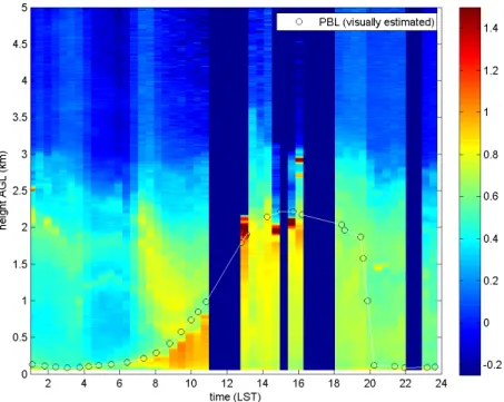
have the greatest influence on modeled vertical profiles. Figure 3.5 shows a time series

of the vertical lidar backscatter profiles on September 7, 2006, with visually estimated

PBL heights indicated by the open circles.

(24)

Figure 3.5: Lidar backscatter image from Moody Tower, TX on September 7, 2006. Warm colors indicate higher concentrations of aerosols and open circles indicate visually estimated PBL heights. (Flynn, 2006)

Figure 3.5 is an example of the extreme variability of the PBL depth in the downtown

Houston area, with dark blue patches throughout the afternoon and evening indicating

the presence of low clouds that suppress PBL growth. Figure 3.6 displays a time series

of the visually analyzed lidar PBL heights on September 7, 2006 along with

radiosonde-derived and modeled PBL heights. As expected, the lidar-radiosonde-derived PBL heights compare

well to those derived from the radiosonde. PBL heights output by the WRF model

show a very steep PBL increase of about 1400m between 1000 and 1200 CST, while

the lidar-derived PBL heights show a similar increase of 1400m between 1000 and

1300 CST. WRF predicted a 2700m deep afternoon peak PBL, compared to the

lidar-derived peak of 2200m and radiosonde-lidar-derived peak of 2100m, while MM5 predicted a

much more shallow afternoon PBL peak of 1660m. The WRF PBL collapsed 2300m

(25)

PBL decrease of 1300m between 1500 and 1800 CST. The lidar data was removed

between 1600 and 1800 CST due to low clouds in the area, though the lidar-derived

PBL heights show a later collapse than both models’ predicted of 1900m between 1830

and 2030 CST.

0 2 4 6 8 10 12 14 16 18 20 22 24

0 500 1000 1500 2000 2500 3000

Time (CST)

PBL Height (m)

WRF Model MM5 Model Lidar Radiosonde

Figure 3.6: Time series of modeled and observed PBL heights on September 7, 2006 at Moody Tower, TX. Open circles indicate visually estimated PBL heights from the lidar backscatter image (Figure 3.5), and green diamonds indicate visually estimated PBL heights from radiosonde profiles (Figure 3.7).

Frequent vertical profiles of potential temperature and humidity through the lowest

few kilometers of the atmosphere are the most direct way to test a PBL model. Several

radiosonde balloons were launched from Moody Tower, TX on September 7, 2006, five

of which were during daytime hours and provide a rare opportunity to evaluate the

vertical profiles predicted by WRF-ACM2 and MM5-Eta at multiple times throughout

the day. Potential temperature and mixing ratio are both conserved within the PBL,

thus finding the point at which a sharp increase in potential temperature and a sharp

decrease in mixing ratio (Nielsen-Gammon et al., 2008b) occur signifies the top of

(26)

the PBL. Figure 3.7(a-e) displays modeled and observed vertical profiles of potential

temperature (left) and mixing ratio (right) at 0900, 1200, 1500, 1800, and 2100 CST.

The horizontal green line on each profile represents the height of the PBL as diagnosed

from the observed profiles (black dots). ! ! ! ! ! ! ! ! ! !

296 298 300 302 304 306 308 310 312 314

0 500 1000 1500 2000 2500 3000

Potential Temperature (K)

Height (m) 0900 CST WRF MM5 OBS OBS PBL

0 2 4 6 8 10 12 14 16 18 20

0 500 1000 1500 2000 2500 3000

Mixing Ratio (g/kg)

296 298 300 302 304 306 308 310 312 314

0 500 1000 1500 2000 2500 3000

0 2 4 6 8 10 12 14 16 18 20 0 500 1000 1500 2000 2500 3000

Mixing Ratio (g/kg)

296 298 300 302 304 306 308 310 312 314

0 500 1000 1500 2000 2500 3000

0 2 4 6 8 10 12 14 16 18 20 0 500 1000 1500 2000 2500 3000

Mixing Ratio (g/kg)

(27)

! ! ! ! ! !"#$%&'()'*&%+",-.'/%01".&2'01'/0+&3+"-.'+&4/&%-+$%&'5.&1+6'-37'4"8"3#'%-+"0'5%"#9+6'-2'%&,0%7&7'1%04'%-7"02037&' :-..0032'.-$3,9&7'-+';007<'=0>&%?'=@'03'A&/+&4:&%'B?'CDDE'-+'5-6'D(DD?'5:6'FCDD?'5,6'FGDD?'576'FHDD?'-37'5&6' CFDD'IA=)'! ! !

296 298 300 302 304 306 308 310 312 314

0 500 1000 1500 2000 2500 3000

0 2 4 6 8 10 12 14 16 18 20 0 500 1000 1500 2000 2500 3000

Mixing Ratio (g/kg)

296 298 300 302 304 306 308 310 312 314

0 500 1000 1500 2000 2500 3000

0 2 4 6 8 10 12 14 16 18 20 0 500 1000 1500 2000 2500 3000

Mixing Ratio (g/kg)

Height (m) 2100 CST WRF MM5 OBS OBS PBL (d) (e)

Figure 3.7: Vertical profiles of potential temperature (left) and mixing ratio (right) as recorded from radiosonde balloons launched at Moody Tower, TX on September 7, 2006 at (a) 0900, (b) 1200, (c) 1500, (d) 1800, and (e) 2100 CST.

At 0900 CST (Figure 3.7a), vertical profiles predicted by WRF-ACM2 and

MM5-Eta shows realistic PBL heights, although both meteorological models under-predicted

moisture at the surface. At 1200 CST (Figure 3.7b), MM5-Eta profiles closely match

observations with a 1200 m deep PBL, while the WRF-ACM2 profile indicates a PBL

height that is about 1700 meters deep, approximately 100 meters higher than the PBL

height output by WRF at 1200 CST, shown in Figure 3.6. The WRF-ACM2 profile

much more closely matched observations at 1500 CST (Figure 3.7c) with a PBL height

of about 2300 m, although the actual WRF output PBL for 1500 CST was about

300 m higher (Figure 3.6). The vertical profile for MM5-Eta at 1500 CST indicates

(28)

a shallower PBL height of about 1500m, and WRF and MM5 under-predicted both

surface temperature and moisture. Figure 3.7d shows the vertical profiles at 1800 CST,

with the MM5-Eta model under-predicting the PBL height by about 600m, although

the actual output PBL by MM5 (Figure 3.6) was 500 m even more shallow than that

predicted by the profile, at a height of only 800 m. The WRF-ACM2 profile indicates

a PBL height of 2300 m at 1800 CST, compared to the radiosonde observed PBL of

about 1900 m, with the actual WRF output PBL being about 2500 m. The 400 m PBL

height diagnosed from the observed vertical profile at 2100 CST (Figure 3.7e) was not

predicted by either model or observed by the lidar backscatter profile (Figure 3.6), but

(29)

Chapter 4 Discussion

The recently developed ACM2 PBL scheme was evaluated for use in regulatory air

quality models in eastern Texas using a spatially and temporally diverse observational

dataset collected during the TexAQS II and TRAMP field campaigns between

Au-gust and October of 2006. Outputs from WRF V3.1 using the ACM2 PBL scheme

were compared with these observations and with outputs from MM5 V3.7.3 using the

Eta PBL scheme, the meteorological model currently being used to develop O3 control

strategies in the HGB area. Both models were given a rigorous test of their ability to

predict realistic PBL heights during daytime convective conditions across varying

ter-rains. Variables that affect PBL height as a result of each model’s land-surface model

were also investigated to determine biases that would not be the fault of each respective

model’s PBL scheme.

The spatially diverse set of RWP-derived PBL heights were used to compare both

model’s ability to predict accurate PBL heights at varying terrains and distances from

the coast. WRF-ACM2 produced more accurate PBL heights than MM5-Eta at all

ten RWP locations and at all periods of the day, with MM5-Eta having the most

trouble predicting accurate daily peak and evening collapse PBL heights at the furthest

inland sites. Time series plots revealed that MM5-Eta was drastically under-predicting

(30)

(Central Texas, Inland, Coastal Plains), whereas the WRF-ACM2 model was slightly

over-predicting the afternoon peak at the Inland and Coastal Plains locations, but also

collapsing the PBL more rapidly than observations for all three regions.

The RWP analysis reveals a major weakness in the MM5-Eta model’s ability to

accurately simulate PBL evolution during convective conditions, a commonly reported

insufficiency of local closure PBL schemes. Alternatively, WRF-ACM2 predicted a

much more accurate PBL evolution, both temporally and spatially, in Eastern Texas.

Inspection of median surface temperature and moisture time series plots revealed higher

surface temperatures in WRF with more surface moisture in MM5, although these could

not be attributed to surface heat fluxes, and thus the differences in performance of the

WRF and MM5 models are likely due to the PBL schemes.

Vertical profiles of temperature and moisture collected from radiosonde balloons on

September 7, 2006 were used to evaluate the PBL schemes in the lowest 3 km of the

at-mosphere. WRF closely matched the rapidly rising PBL indicated by the lidar-derived

PBL heights, while MM5 predicted a more slowly rising and shallow PBL not

represen-tative of the daytime urban boundary layer. WRF’s close comparisons to radiosonde

profiles at five times during the day during mostly clear, low wind conditions further

validate ACM2’s ability to accurately represent the PBL during daytime convective

(31)

Chapter 5 Conclusions

An accurate depiction of the diurnal evolution and vertical mixing within the PBL is

necessary for realistic air quality simulations. For the current meteorological modeling

in support of HGB O3 attainment demonstration, TCEQ chose the Eta PBL scheme,

a local closure TKE model shown in this study to be inadequate at representing the

daytime convective boundary layer. Eastern Texas is characterized by a considerable

spatial variability of PBL height due to its coastal location and variations in land use,

and thus requires a PBL scheme that can more accurately represent this variability.

The recently developed combined local and nonlocal closure ACM2 PBL scheme was

shown here to accurately simulate the morning growth, maximum height, and evening

decay of the daytime PBL across varying regions in eastern Texas, while producing

realistic vertical profiles of temperature and moisture at Moody Tower in downtown

(32)

Bibliography

Banta, R., Seniff, C., Nielsen-Gammon, J., Darby, L., Ryerson, T., Alvarez, R., Sand-berg, S., Williams, E., Trainer, M., 2005. A bad air day in houston. B Am Meteorol Soc 86, 657–669.

Blackadar, A. K., 1978. Modeling pollutant transfer during daytime convection. Preprints, Fourth Symposium on Atmospheric Turbulence, Diffusion, and Air Pollu-tion, Reno, NV, Amer. Meteor. Soc., 443–447.

Brown, A. R., 1996. Evaluation of parameterization schemes for the convective bound-ary layer using large-eddy simulation results. Bound-Lay Meteorol 31, 167–200.

Byun, D. W., Pleim, J. E., Tang, R. T., Bourgeois, A., 1999. Meteorology-chemistry interface processor (mcip) for models-3 community multiscale air quality (cmaq) modeling system. Office of Research and Development, US Environmental Protection Agency, Research Triangle Park, NC.

Dabberdt, W. F., Carroll, M. A., Baumgardner, D., Carmichael, G., Cohen, R., Dye, T., Ellis, J., Grell, G., Grimmond, S., Hanna, S., Irwin, J., Lamb, B., Madronich, S., McQueen, J., Meagher, J., Odman, T., Pleim, J., Schmid, H. P., Westphal, D. L., 2004. Meteorological research needs for improved air quality forecasting: Report of the 11th prospectus development team of the u.s. weather research program. B Am Meteorol Soc 85, 563–586.

Darby, L., 2005. Cluster analysis of surface winds in houston, texas, and the impact of wind patterns on ozone. J Appl Meteorol 44, 1788–1806.

Ek, M. B., Mitchell, K. E., Lin, Y., Rogers, E., Grunmann, P., Koren, V., Gayno, G., Tarpley, J. D., 2003. Implementation of noah land surface model advances in the national centers for environmental prediction operational mesoscale eta model. J. Geophys. Res. 108.

Flynn, C. J., 2006. Tramp nocturnal mixing from micropulse lidar measurements (tn-mpl) final report. TERC Project H-81.

Grell, G., Dudhia, J., Stauffer, D., for Atmospheric Research. Mesoscale, N. C., Dici-sion, M. M., 1994. A description of the fifth-generation penn state/ncar mesoscale model (mm5).

Hu, X.-M., Nielsen-Gammon, J. W., Zhang, F., Sep 2010. Evaluation of three planetary boundary layer schemes in the wrf model. J Appl Meteorol Clim 49 (9), 1831–1844.

(33)

Janjic, Z., 1994. The step-mountain eta coordinate model: Further developments of the convection, viscous sublayer, and turbulence closure schemes. Mon Wea Rev 122, 927–945.

Kain, J., Jan 2004. The kain-fritsch convective parameterization: An update. Journal of Applied Meteorology 43 (1), 170–181.

Knoderer, C. A., MacDonald, C. P., Aug 2007. Texaqs-ii radar wind profiler, radio acoustic sounding system, sodar, and lidar data quality control and mixing height derivation, 1–22.

Ku, J., Mao, H., Zhang, K., Civerolo, K., Rao, S., Philbrick, C., Doddridge, B., Clark, R., 2001. Numerical investigation of the effects of boundary-layer evolution on the predictions of ozone and the efficacy of emission control options in the northeastern united states. Environ Fluid Mech 1 (2), 209–233.

Lefer, B., Rappengl¨uck, B., 2010. The texaqs-ii radical and aerosol measurement project

(tramp). Atmos Environ 44 (33), 3997–4004.

Mlawer, E., Taubman, S., Brown, P., Iacono, M., Clough, S., 1997. Radiative trans-fer for inhomogeneous atmospheres: Rrtm, a validated correlated-k model for the longwave. J. Geophys. Res. 102, 16663–16682.

Morrison, H., Gettelman, A., 2008. A new two-moment bulk stratiform cloud micro-physics scheme in the community atmosphere model, version 3 (cam3). part i: De-scription and numerical tests. Journal of Climate 21 (15), 3642–3659.

Nielsen-Gammon, J., Tobin, J., Bliujus, S., Myoung, B., McRoberts, B., 2008a. Terc project h84: Development of databases and charaterization of meteorological condi-tions for the texaqs ii intensive period, 1–55.

Nielsen-Gammon, J. W., Powell, C. L., Mahoney, M. J., Angevine, W. M., Senff, C., White, A., Berkowitz, C., Doran, C., Knupp, K., 2008b. Multisensor estimation of mixing heights over a coastal city. J Appl Meteorol Clim 47 (1), 27–43.

Otte, T., Pleim, J., 2010. The meteorology-chemistry interface processor (mcip) for the cmaq modeling system: updates through mcipv3.4.1. Geoscientific Model Develop-ment 3, 243–256.

Parrish, D. D., Allen, D. T., Bates, T. S., Estes, M., Fehsenfeld, F. C., Feingold, G., Ferrare, R., Hardesty, R. M., Meagher, J. F., Nielsen-Gammon, J. W., Pierce, R. B., Ryerson, T. B., Seinfeld, J. H., Williams, E. J., 2009. Overview of the second texas air quality study (texaqs ii) and the gulf of mexico atmospheric composition and climate study (gomaccs). J. Geophys. Res. 114.

P´erez, C., Jim´enez, P., Jorba, O., Sicard, M., 2006. . . . the pbl scheme on high-resolution photochemical simulations in an urban coastal area over . . . . Atmos Env-iron 40 (27), 5274–5297.

(34)

Pleim, J., 2006. A simple, efficient solution of flux-profile relationships in the atmo-spheric surface layer. J Appl Meteorol Clim 45 (2), 341–347.

Pleim, J., 2007a. A combined local and nonlocal closure model for the atmospheric boundary layer. part i: Model description and testing. J Appl Meteorol Clim 46 (9), 1383–1395.

Pleim, J., 2007b. A combined local and nonlocal closure model for the atmospheric boundary layer. part ii: Application and evaluation in a mesoscale meteorological model. J Appl Meteorol Clim 46 (9), 1396–1409.

Pleim, J., Chang, J., 1992. A non-local closure model for vertical mixing in the convec-tive boundary layer. Atmos Environ. Part A. General Topics 26 (6), 965–981.

Rappengl¨uck, B., Perna, R., Zhong, S., Morris, G. A., 2008. An analysis of the vertical

structure of the atmosphere and the upper-level meteorology and their impact on surface ozone levels in houston, texas. J. Geophys. Res. 113.

Seaman, N., 2000. Meteorological modeling for air-quality assessments. Atmos Environ 34 (12-14), 2231–2259.

Skamarock, W. C., Klemp, J. B., Dudhia, J., Gill, D. O., Barker, D. M., Duda, M., Huang, H., Wang, W., Powers, J. G., 2008. A description of the advanced research wrf version 3, 1–125.

TCEQ, Mar 2010. Revisions to the state implementation plan for the control of ozone air pollution, houston-galveston-brazoria 1997 eight-hour ozone standard nonattain-ment area, 1–152.

URL http://www.tceq.texas.gov/implementation/air/sip/HGB_eight_hour. html

Vizuete, W., Jeffries, H., Christoph, E., 2008. Harc project h87 (unc) multi-resolution simulation and analysis of texaqs ii air . . . . files.harc.edu.

Wilczak, J. M., Djalalova, I., McKeen, S., Bianco, L., Bao, J.-W., Grell, G., Peckham, S., Mathur, R., McQueen, J., Lee, P., 2009. Analysis of regional meteorology and surface ozone during the texaqs ii field program and an evaluation of the nmm-cmaq and wrf-chem air quality models. J of Geophys Res-Atmos 114, D00F14.

Xiu, A., Pleim, J., 2001. Development of a land surface model. part i: Application in a mesoscale meteorological model. Journal of Applied Meteorology 40 (2), 192–209.