Geometric Collision Avoidance for Heterogeneous Crowd
Simulation
Stephen J. Guy
A dissertation submitted to the faculty of the University of North Carolina at Chapel Hill in partial fulfillment of the requirements for the degree of Doctor of Philosophy in the Department of Computer Science.
Chapel Hill 2012
ABSTRACT
STEPHEN J. GUY: Geometric Collision Avoidance for Heterogeneous Crowd Simulation (Under the direction of Ming C. Lin and Dinesh Manocha)
Simulation of human crowds can create plausible human trajectories, predict likely flows of pedestrians, and has application in areas such as games, movies, safety planning, and virtual environments. This dissertation presents new crowd simulation methods based on geometric techniques. I will show how geometric optimization techniques can be used to efficiently compute collision-avoidance constraints, and use these constraints to generate human-like trajectories in simulated environments. This process of reacting to the nearby environment is known aslocal navigationand it forms the basis for many crowd simulation techniques, including those described in this dissertation.
Given the importance of local navigation computations, I devote much of this disser-tation to the derivation, analysis, and implemendisser-tation of new local navigation techniques. I discuss how to efficiently exploit parallelization features available on modern proces-sors, and show how an efficient parallel implementation allows simulations of hundreds of thousands of agents in real time on many-core processors and tens of thousands of agents on multi-core CPUs. I analyze the macroscopic flows which arise from these geometric collision avoidance techniques and compare them to flows seen in real human crowds, both qualitatively (in terms of flow patterns) and quantitatively (in terms of flow rates).
data to automatically tune parameters, and using perceptual user study data to introduce behavioral variation.
Finally, looking beyond geometric avoidance based crowd simulation methods, I discuss methods for objectively evaluating different crowd simulation strategies using statistical measures. Specifically, I focus on the problem of quantifying how closely a simulation approach matches real-world data. I propose a similarity metric that can be applied to a wide variety of simulation approaches and datasets.
ACKNOWLEDGEMENTS
There are many people who, through support, kindness, and constructive conflict, have contributed a great deal to my research in graduate school and eventually this thesis. First and foremost, I want to thank my advisors Ming Lin and Dinesh Manocha who have both been a constant source of guidance throughout my entire six years here. Ming and Dinesh were some of the first faculty I met at UNC and have, at every point, pushed me to accomplish as much as possible during my time in the department. I have also benefited greatly from my committee members: Lana Lazebnik for teaching me virtually everything I know about computer vision and machine learning, Marc Niethammer for great discussions on optimization theory, and Jatin Chhugani whose world class expertise on computer architecture and practical approach to conducting research has left a positive impact on every project I have worked on since meeting him.
I will also be forever indebted to two amazing mentors: Leonid Zhigilei for introducing me to the world of university research, and Pradeep Dubey for showing me the best of what is possible at an industrial lab. My work at their respective labs inspired my desire for research and contributed directly to the material presented here.
I would additionally like to thank Jur P. van den Berg, both for his cheerful mentorship and for introducing me to RVO – which would forever change my research career. I’ve also been blessed with a large supply of collaborators in my research: Sujeong Kim, Sahin Patil, Sean Curtis, Jamie Snape, Rahul Narain, and Wenxi Liu, any use of the word ‘I’ in this document likely reflects a great deal of contribution from these people.
TABLE OF CONTENTS
LIST OF TABLES . . . xvi
LIST OF FIGURES . . . .xviii
LIST OF ABBREVIATIONS . . . xxv
1 Introduction . . . 1
1.1 Crowd Simulation Overview . . . 2
1.1.1 Defining the Scenario . . . 2
1.1.2 Computing Crowd Motion. . . 4
1.1.3 Animating and Rendering of Crowds. . . 5
1.2 Motion in Crowds . . . 6
1.2.1 Heterogeneous Crowd Simulations. . . 6
1.2.2 Global Navigation . . . 7
1.2.3 Velocity Space Planning for Local Navigation . . . 8
1.3 Modern Processor Architecture Trends . . . 9
1.4 Thesis statement. . . 10
1.5 Main Results . . . 11
1.5.1 Parallel, Optimization-Based Collision Avoidance . . . 11
1.5.2 Crowd Simulation based on the Principle of Least Effort . . . 12
1.5.3 Data Use in Crowd Modeling . . . 13
1.5.4 Simulation Validation form Real-World Data . . . 13
2 ClearPath: A Method for Decentralized Collision Avoidance . . . 15
2.1 Introduction . . . 15
2.1.1 Main Results . . . 16
2.1.2 Organization. . . 17
2.2 Previous Work . . . 17
2.2.1 Collision detection and path planning . . . 17
2.2.2 Collision avoidance . . . 18
2.2.3 Parallel algorithms . . . 19
2.3 Local Collision Avoidance . . . 19
2.3.1 Velocity Obstacles . . . 20
2.3.2 Optimization Formulation for Collision Avoidance . . . 22
2.3.3 ClearPath Implementation . . . 24
2.4 P-ClearPath: Parallel Collision Avoidance . . . 26
2.5 Implementation and Results . . . 30
2.5.1 Behavior Evaluation . . . 33
2.5.2 Complex Scenarios . . . 34
2.5.3 Parallel Implementation . . . 34
2.5.3.1 Data-Parallelism . . . 35
2.5.3.2 Thread-level Parallelism (TLP) . . . 36
2.5.3.3 SIMD Scalability. . . 37
2.6 Analysis and Comparisons . . . 38
2.6.1 Performance Analysis . . . 38
2.6.2 Behavioral Analysis. . . 38
2.6.3 Comparison and Limitations. . . 39
2.7 Conclusions and Future Work . . . 41
2.7.1 Limitations . . . 41
2.8 ORCA . . . 42
3 PLEdestrians: A Caloric-Minimization Approach to Crowd Simulation . . . 44
3.1 Introduction . . . 44
3.1.1 Main Result . . . 45
3.1.2 Organization. . . 45
3.2 Previous Work . . . 45
3.2.1 Least Effort in Crowd Simulation . . . 46
3.2.2 Motion Synthesis . . . 46
3.3 PLE Model . . . 47
3.3.1 Notation and Overview . . . 47
3.3.2 Least Effort Function . . . 48
3.3.3 Mathematical Model for Effort Minimization . . . 50
3.3.4 Properties of the PLE Metric . . . 51
3.4 Trajectory Computation. . . 52
3.4.1 Algorithm Overview . . . 52
3.4.2 Dynamic Energy Roadmap . . . 53
3.4.3 Velocity Computation . . . 54
3.4.4 Clustering-based Optimizations. . . 56
3.5 Results. . . 57
3.5.1 Benchmarks . . . 57
3.5.2 Comparison to Other Methods . . . 59
3.5.3 Comparison to Data from Crowd Studies . . . 61
3.5.4 Performance Results . . . 65
3.6 Analysis . . . 65
3.7 Summary and Conclusions . . . 66
3.7.2 Future Work . . . 67
4 PLE Simulation Approach: Analysis and Validation . . . 69
4.1 Introduction . . . 69
4.1.1 Main Result . . . 69
4.1.2 Organization. . . 70
4.2 Previous Work . . . 70
4.3 Least-Effort Model . . . 72
4.3.1 Optimization Formulation . . . 74
4.3.2 Geometric Solution . . . 75
4.3.3 Global Navigation . . . 77
4.4 Results. . . 78
4.4.1 Emergent Phenomena . . . 78
4.4.2 Flow Analysis . . . 80
4.4.3 Path Comparison . . . 82
4.4.4 Complex Scenarios . . . 83
4.5 Summary and Conclusions . . . 84
4.5.1 Limitations . . . 85
4.5.2 Future Work . . . 85
5 Data-driven Simulation of Variations in Human Trajectories . . . 86
5.1 Introduction . . . 86
5.1.1 Main Result . . . 86
5.1.2 Organization. . . 87
5.2 Background and Previous Work . . . 87
5.2.1 Multi-robot Collision Avoidance . . . 87
5.2.2 Modeling Human Motion . . . 88
5.3 Distributed Collision Avoidance . . . 89
5.3.1 Velocity Obstacles . . . 90
5.3.1.1 Reciprocal Collision Avoidance . . . 92
5.3.2 Optimization Formulation . . . 92
5.3.2.1 Multi-agent Collision Avoidance . . . 93
5.4 Reciprocal Collision Avoidance for Pedestrians . . . 94
5.4.1 Modeling Human Motion . . . 94
5.4.1.1 Response and Observation Time . . . 95
5.4.1.2 Kinodynamic Constraints . . . 95
5.4.1.3 Personal Space . . . 96
5.4.2 Static Obstacles and Global Navigation . . . 97
5.4.3 Algorithm Overview . . . 98
5.5 Model Optimization & Training . . . 98
5.5.1 Training Approach . . . 100
5.5.1.1 Optimization Metric . . . 100
5.5.2 Optimal RCAP Values . . . 102
5.5.3 RCAP Parameter Distribution . . . 104
5.6 Model Validation . . . 105
5.6.1 Collision Response Phases . . . 106
5.6.2 Biomechanical Energy Consumption Analysis . . . 107
5.6.3 Path Similarity . . . 107
5.6.4 Cross Validation . . . 108
5.7 Simulation Results . . . 109
5.7.1 Multi-person Simulations . . . 109
5.7.1.1 Data-driven Crowd Simulations . . . 110
5.8 Comparison & Analysis . . . 111
5.8.2 Simulation Analysis. . . 113
5.8.2.1 Behavioral Analysis . . . 113
5.8.2.2 Performance Analysis . . . 113
5.8.3 Comparison to Other Methods . . . 114
5.9 Summary and Conclusions . . . 116
5.9.1 Limitations . . . 116
5.9.2 Future Work . . . 117
6 Data-driven Simulation of Variations in Personality . . . 119
6.1 Introduction . . . 119
6.1.1 Main Result . . . 120
6.1.2 Organization. . . 121
6.2 Previous Work . . . 121
6.2.1 Human Behavior Modeling . . . 121
6.2.2 Modeling Crowd Styles . . . 122
6.3 Personality Models and Trait Theory . . . 122
6.3.1 Trait Theory . . . 122
6.3.2 Factor Analysis . . . 123
6.4 Behavior Perception User Study . . . 124
6.4.1 Method. . . 125
6.5 Data Analysis . . . 128
6.5.1 Mapping Perceived Behaviors . . . 128
6.5.2 Mapping Parameters for the PEN Model . . . 129
6.5.3 Factor Analysis . . . 130
6.6 Simulation Results and Validation Study . . . 131
6.6.1 Simulation Results . . . 132
6.6.3 Timing Results . . . 136
6.6.4 Validation Study . . . 137
6.7 Summary and Conclusions . . . 140
6.7.1 Limitations . . . 140
6.7.2 Future Work . . . 141
7 An Entropy Metric for Evaluating Crowd Simulations . . . 144
7.1 Introduction . . . 144
7.1.1 Main Result . . . 145
7.1.2 Organization. . . 146
7.2 Background and Notation . . . 146
7.2.1 Definitions . . . 146
7.2.2 Crowd Simulation and Trajectory Generation . . . 147
7.2.3 Crowd Data Sources . . . 149
7.3 Entropy Metric . . . 149
7.3.1 Computing the Entropy Metric . . . 151
7.3.2 Simplifying Assumptions . . . 152
7.3.3 Computing Crowd State Distributions . . . 154
7.3.4 Computing the VarianceM. . . 154
7.3.5 Computing the Entropy ofM . . . 156
7.4 Implementation and Experimental Set-up . . . 157
7.4.1 Simulation Models . . . 157
7.4.2 Real-World Crowd Data . . . 158
7.5 Analysis and Comparisons . . . 160
7.5.1 Metric Properties . . . 161
7.5.2 Consistency . . . 162
7.5.3 Comparison with Prior Approaches . . . 165
7.6 Summary and Conclusions . . . 166
7.6.1 Limitations . . . 166
7.6.2 Future Work . . . 167
8 Conclusion . . . 168
8.1 Limitations. . . 169
8.2 Future Work . . . 171
A ClearPath Derivations and Proofs . . . 173
A.1 Derivation of AB(v). . . 173
A.2 Derivation of AB(v). . . 174
A.3 Proof of Lemma 1 . . . 174
A.4 Proof of Lemma 2 . . . 175
A.5 Proof of Theorem 1. . . 175
B PLEdesrian Derivations and Proofs . . . 176
B.1 Proof of Lemma 1 (Nature of Min. Energy Path) . . . 176
B.2 Objective Function of Eqn. 3.4 is a convex function . . . 176
B.3 Minima of Eqn. 3.4 lies on the boundary ofP VA. . . 177
B.4 Proofs of Lemma 2 and Lemma 3 . . . 177
LIST OF TABLES
2.1 Average time (%) spent in various steps (Section 3.3) of Clearpath and the corresponding SIMD scalability on Larrabee simulator of
execution cycles as compared to the scalar version. . . 37
3.1 Energy expended and simulated time to complete the benchmark for 2-Agent swapping (#1), 10-Agent Circle (#2) and Concentric Circles (#3). *OpenSteer fails to avoid collisions in the dense regions of this scenario. . . 61
3.2 Performance Results for different benchmarks. The algorithm scales almost linearly with the number of cores. . . 65
5.1 Variables of state for each agent . . . 90
5.2 Table of RCAP constants. . . 102
5.3 Variance of RCAP parameters between participants.. . . 104
6.1 Range of simulation parameters. . . 127
6.2 Excerpt from the mapping between adjectives and PEN factors given in (Pervin, 2003) and used createApen. . . 129
6.3 Simulation parameters for various personality traits. . . 133
6.4 Performance timings per frame. . . 136
6.5 Performance on validation study . . . 139
7.1 Summary of real-world crowd datasets used in this work. . . 159
7.2 Entropy metric for different simulation algorithms on various datasets. . . 160
7.3 The entropy metric results on similar datasets such as (Passage-1,Passage-2) or (Street-1,Street-2) are highly correlated. The metric shows lower correlation for different dataset pairs. . . 162
7.5 As the accuracy of the RVO algorithm is improved based on the data from Lab benchmark, the entropy metric decreases. RVO-A is the worst algorithm for this benchmark and RVO-D is the best algorithm. There is a direct correlation between the entropy metric
LIST OF FIGURES
1.1 Still from a visualization of a simulation of the Tawaf ritual. Agents receive a desired velocity from a flow field directing them in a
counterclockwise motion around the Kabah (central structure). . . 4
1.2 ClearPath performing collision avoidance on several large-scale
scenarios with hundreds of agents at varying densities. . . 12 1.3 Images of various crowd simulations using ideas inspired by
biome-chanics research. The simulations show a variety of emergent
phenomena such as lane formation. . . 13 1.4 (a) Data-driven crowd simulations (b-c) Data-driven evaluation scenarios . . . 14
2.1 The Velocity ObstacleV OA
B(vB)of a disc-shaped obstacleBto a disc-shaped agentA. This VO represents the velocities that could
result in a collision ofAwithB(i.e. potentially colliding region). . . 21 2.2 The Finite-time horizon Velocity Obstacle FVOA
B(vB) of a disc-shaped obstacleB to a disc-shaped agentA. This formulation takes
into account the time interval for local collision avoidance. . . 22
2.3 Classifying FVO boundary subsegments as Inside/Outside of the remaining FVO regions for multi-agent simulation. The optimiza-tion algorithm performs these classificaoptimiza-tion tests to compute a
non-colliding velocity for each agent.. . . 24 2.4 Red lens area: Velocities which will not remove agent from
col-lision this time-step. Green cone: Conservative conical approxi-mation of red area. CircleR: Minkowski sum of colliding agents.
CircleP: Positions current agent can reach next time step. . . 27
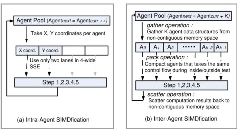
2.5 Data-Parallel Computations: (a) Intra-Agent SIMDfication for SSE
(b) Inter-Agent SIMDfication for wide SIMD . . . 28 2.6 For each agent, each time step, ClearPath takes a desired velocity
from a multi-agent simulation, and a list of nearby neighbors and computes a new minimally perturbed velocity with avoids collisions.
This velocity is then used as the agent’s new velocity. . . 30
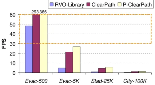
2.7 Performance of RVO-Library, ClearPath and SSE implementation of P-ClearPath measured on a single core Xeon. The ClearPath implementation is about 5X faster than RVO-Library. The SSE
2.8 Dense Circle Scenario:1,000agents are arranged uniformly around
a circle and move towards their antipodal position. This simulation runs at over 1,000 FPS on an Intel 3.14 GHz quad core, and over
8,000 FPS on 32 Larrabee cores. . . 33
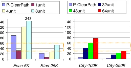
2.9 Performance (FPS) of P-ClearPath on SSE (left most column) and Larrabee (with different units) architectures. Even on complex
scenes, P-ClearPath achieves30 60FPS on many-core processors. . . 36
2.10 A snapshot of the 80 agent Back&Forth demo. Opensteer (on the left) averages 16 collisions per frame. When combined with ClearPath (on the right) the simulation is collision-free. Two
partic-ularly egregious collision are circled in red. . . 39
2.11 As density increases, OpenSteer’s collision rate increase super-linearly. Simply using ClearPath on it’s own, and combining
Open-Steer with ClearPath results in practically no collisions. . . 40
2.12 Constructing the set of ORCA allowed velocities. voptis the agent’s current velocity. ORCA forces agents to choose new velocities which avoid at least half the collision u. In RCAP, only agents
whoseTsightB|A < T TobsgenerateORCAconstraints. . . 43 2.13 Still from a real-time, ORCA simulation of Tawaf ritual involving
25,000 agents. . . 43
3.1 The algorithm computes the new velocity (vnew
A ) for moving from
pAtoGAin accordance with PLE. The effort function is analyti-cally minimized over all possible intermediate positionsqA, such
that the the agent expends least amount of effort to reach its goal. . . 50
3.2 Multi-agent navigation: An overview of the proposed approach for computing the trajectory for each agent. Each agent performs these computations at each time step. The roadmap used for navi-gation is also updated. The effort function shown in Eq. 3.4 is used
by the optimization algorithm for velocity computation. . . 52
3.3 Velocity selection - (a) Agent A avoids 4 neighboring agents. (b) The permissible velocitiesP VAof agentAis shown in white. Ra-diating ellipses correspond to iso-contours of the energy function. The circles show the local minima along each line segment, the en-larged white circle being the global minima of the energy function and the new velocity computed for this agent for the next time step,vnew
A . . . . 54 3.4 Long Corridor Scenario . . . 57
3.6 Narrow Passage Scenario . . . 58
3.7 A simulation frame from the Trade Show Floor consisting of1,000
agents. PLEdestrians computes collision-free trajectories with
many emergent behaviors at 31 fps. . . 59
3.8 Simulation of Shibuya Metro Station . . . 60
3.9 Comparisons of path traced for 2-Agent Crossing: The figure shows the initial position (star) and final position (circle) for each agent, along with a comparison of the paths traced by PLEdestrians (blue) and Helbing social force algorithm (red). PLEdestrians paths
have less deviation and consume less total effort for the agents. . . 61
3.10 Effect of density on the speed. This graph compares the results of PLEdestrians with the prior data collected on real humans. The
PLE model matches real-world data closely. . . 62
3.11 Edge-Effect Phenomena. A graph of speed vs. a cross section of the PLEdestrian simulation. Agents near the edge of the crowd
move faster than those in the center. . . 63
3.12 Effect of PLE on Congestion:A comparison of the effort of each agent in PLEdestrians vs. ClearPath and RVO in the trade-show benchmark. The PLEdestrian approach avoids congestion and there is only a slow increase in the average effort that is needed to reach
the goals as the number of agents increases. . . 64
4.1 Graph of the empirical relationship between velocity and caloric efficiency for adult males (Whittle, 2002) (Eq. 4.1). The minimum energy corresponds to the velocity 1.3 m/s, the average walking
velocity for adult males. (Kl¨upfel et al., 2005). . . 73
4.2 Computation Overview. The current agent, A1, has a goal marked X,
but needs to avoid two approaching agents,A2andA3, each with some velocity (arrows). Each neighbor creates a restriction on the velocity the current agent can take (boundary line and shaded regions show forbidden endpoints of the velocity vector ofA1), leaving the set of collision-free
permissible velocities (PV). Each velocity results in some expected energy to reach the goal (dashed ellipses mark the iso-contours of this function). The computed new velocity (light arrow) is the one which leads to the collision-free path to the goal (dotted line) using the least expected energy. This model is used to compute a new velocity for each agent at each
4.3 Lane Formation. (a) Two opposing groups of agents, (dark) red and (light) blue, have opposing initial conditions with goals past each other. (b) As the groups approach the agents naturally form into
small coherent lanes reducing the overall effort of each individual. . . 78
4.4 Stills from a simulation of humans walking through a narrow pas-sage, taken at 15 second intervals. There is initially jamming at the passage (a), followed by a semi-circular arch forming around the exit (b). Once through the passage, individuals do not immediately
spread out, but leave an empty space or “wake” behind the obstacles (c). . . 79 4.5 Flow Analysis Scenario. 96 agents are placed in a room of
dimen-sion 5m x 8m. Agents are given a goal outside the room which requires them to pass through the exit on the right wall. The ex-periment is repeated for various exit widths varying from 0.8m to
1.4m. . . 80
4.6 Real and Simulated Flow Rates. A comparison of the effect of exit width on the flow for real (dashed lines) and simulated (solid line) humans. Agents simulated with the PLE model exhibit similar flow
as real humans. . . 81 4.7 The fundamental diagram comparing agent speeds vs their local
density (solid line) matches the relationship established by
Weid-mann (dashed line) (WeidWeid-mann, 1992). . . 82 4.8 Paths of two humans passing each other. The model’s path (light
solid line) matches very closely with the the mean of the human paths (dark solid line), and within one standard deviation of human
paths (dashed lines). . . 83
4.9 Paths taken past a static obstacle (circle). The model’s path (light solid line) matches very closely with the the mean of the human paths (dark solid line), and within one standard deviation of human
paths (dashed lines). . . 83 4.10 The PLE approach automatically generates many emergent crowd
behaviors at interactive rates in this simulation of Shibuya Crossing (left) that models a busy crossing at the Shibuya Station in Tokyo, Japan. (right). The trajectory for each agent is computed based on
minimizing an biomechanically-inspired effort function. . . 84
5.1 (a) Shows the positions of two agentsAandB, with zero relative velocity. (b) Shows the VO in A’s velocity space induced byB. This is the set of all ofA’s velocities which would collide withB
5.2 Constructing the set of ORCA allowed velocities. voptis the agent’s current velocity. ORCA forces agents to choose new velocities which avoid at least half the collision u. In RCAP, only agents
whoseTsightB|A < T TobsgenerateORCAconstraints. . . 93 5.3 Comparison of a tight oval bounds on the physical space (blue oval)
to the larger personal space which is used for planning (dashed circle). . . 97
5.4 Experimental set-upTwo people (red circles) are placed in a 15m x 15mmotion-tracked lab. Participants start at randomly selected corners, initially unable to see each other due to 5mlong barriers (blue rectangles). They were simultaneously asked to walk to the opposite corner. A few meters into their path they enter the Interaction Areaand can see the other participant and react to avoid
colliding. (Drawn to Scale) . . . 100
5.5 Graph of how the distance between the agents at projected closest point between two agents’ trajectories changes over time during a single trial.Blue Line: Two real people initially start on a colliding path (if unchanged, their centers would be only .1mapart). As the experiment progresses, the people eventually sort out the collision and adopt velocities which will have their centers pass .7mapart, more than far enough to avoid a collision (at least .5m).Green Line:
An RCAP simulation initialized with the above conditions. . . 102
5.6 Closest Approach Graphs for 2 different runs.. . . 103
5.7 The participants’ desired velocities do not lead to a collision course, the real and virtual agents both chose to maintain their desired
velocities, instead of changing them. . . 103
5.8 Distribution ofTobs across all runs. . . 105 5.9 Distribution ofamax, andracross all runs. . . 105 5.10 Comparison of the true collision response curve (Blue Line) to the
one predicted by RCAP with generic constants (Green Line) and
the prediction with constants tuned to the specific runs (Red Line). . . 106
5.11 A comparison of paths Real Humans vs Virtual Humans. Agents are displayed as circles with their goal for this simulation run show in Xs. The redline shows the path that the simulated humans took,
and the black line shows the path of the humans. . . 108 5.12 Comparisons of paths Real Humans vs Virtual Humans from two
additional runs.Black lines: Real humans’ paths,Red lines: Virtual
5.13 Time-lapse diagram of agent positions. (a) Two RCAP agents exchange positions. The agents reciprocate, each taking half the re-sponsibility. (b) A wall prevents the green agent from turning away from the collision. The red agent automatically accommodates,
eventually taking full responsibility for avoiding the collision. . . 110
5.14 Trace of a 6 agent simulation. Agents follow smooth, simple,
curved paths similar to those from the trials with humans. No agents collide. 111
5.15 Snapshot from a simulation of 1,000 people evacuating an office environment.112
5.16 A Comparison of RCAP, ORCA, and Helbing Social Force Model
to real human data during a single trial. . . 115
6.1 Three crowd simulation scenarios. (a) Four highlighted agents move through crowd. (b) Four highlighted individuals move through groups of still agents. (c) 20 highlighted individuals compete with
others to exit through a narrowing passage. . . 126 6.2 This chart shows which behavior adjective has the largest change
as the two principal components are varied. . . 132
6.3 Pass-through Scenario.Paths of agents trying to push through a crowd in various simulations. The agent’s parameters correspond to various personalities. All paths are displayed for an equal length of time. (a) Aggressive agents make the most progress with the straightest paths. (b) Impulsive agents move quickly but take less direct routes. (c) Shy agents are diverted more easily in attempts to avoid others (d) Tense agents take less jittery paths, but are easily
deflected by the motion of others. . . 134
6.4 Hallway Scenario. A comparison between (a) agents with high levels of “Psychoticism”, (b) “Extraversion” and (c) “Neuroticism”. Each of the four agents’ paths is colored uniquely. The high P-factor agents repeatedly cut close to others taking the most direct paths. The high E-factor agents take faster and occasionally “daring” paths, the high N-factor agents take more indirect paths and keep their
distance from others. . . 135
6.5 Narrowing Passage Scenario. A comparison between dark-blue default agents and light-red Aggressive agents (a) and light-red Shy agents (b). The Aggressive agents exited more quickly, while
several Shy agents stay back from the exit causing less congestion.. . . 136 6.6 Exit Rate.Rate at which agents of various personalities exit in the
6.7 Faster-is-slower behavior.This graph shows the speed of Aggres-sive agents exiting in the Narrowing Passage scenario (solid blue line). As a larger percentage of agents become aggressive, their ability to exit quickly is reduced to the point where they exit more slowly than less Aggressive agents with the same preferred speed (dashed red line). This result is consistent with the well-known
“faster-is-slower behavior” (Helbing et al., 2000). . . 138
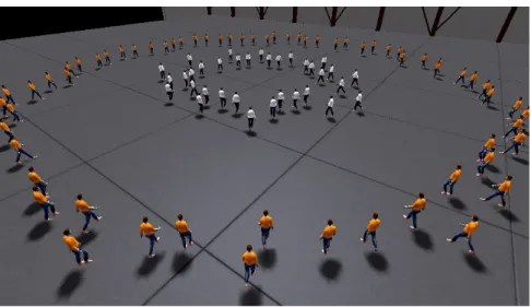
6.8 Evacuation Scenario. 200 agents evacuating a building. Shy agents (brown shirts) hold back while Aggressive agents (red shirts) dart forward. The other personalities also display a variety of
behaviors such as quick maneuvers, overtaking and pushing through. . . 142
6.9 Adjective Success Rate. Rate at which user responses matched the indented adjective for all questions involving the six personality
adjectives studied.⇤indicates statistically significant (p<.05). . . . 143
6.10 PEN Success Rate. Rate at which user responses matched the intended personality trait for questions involving the PEN traits.
⇤indicates statistical significant (p<.05). . . . 143
7.1 Adding a corrective vector mk (green arrow) to each simulation prediction (red dot) can correctly produce true states of the crowd
xk(black dots). The true evolution of the state is shown in black as agents evolve from statex0 tox4. At each timestep, the crowd simulationˆfis used to predict the next state (red dots). In order to reproduce the true state, it is necessary that some correction vector,
mk, is applied at each timestep (green arrow). The distribution of
thesemk’s is denoted asM(dashed ellipse) and contains the true state. . . 150
7.2 The error distribution M for crowd simulation algorithm is es-timated via an iterative process, based on the EM-algorithm. A Bayesian Smoother is used to estimate the true crowd states X
given dataz, a simulatorf, and an error distributionˆ M. Next, the maximum likelihood estimate ofMgiven the simulator is
com-puted and used to estimate the state distributionsX. This process
is repeated until convergence. . . 152 7.3 Rendering of real-world crowd trajectories used for evaluation . . . 160
7.4 The impact of artificial error (uniformly distributed) on the Street-1 benchmark for different algorithms. The entropy metric is stable to this error and the relative ranking of different algorithms does not
change. . . 163
LIST OF ABBREVIATIONS
CA Cellular Automata
FVO Finite-time horizon Velocity Obstacle GPS Global Position Systems
LiDAR Light Detection And Ranging
ORCA Optimal Reciprocal Collision Avoidance PLE Principle of Least Effort
RVO Reciprocal Velocity Obstacle VO Velocity Obstacle
CHAPTER 1
Introduction
Building good models of human crowds is important to many fields such as social science, statistical physics, fire safety planning, and other areas of science and engineering. These models help us gain an understanding of crowds and can facilitate growth, develop more effective societies and cities, and can lead to safer cultural activities and events. By using these models to virtually test design possibilities it is possible to save time, money, and other resources. Devising such models requires us to draw upon developments from various fields which study crowds ranging from sociology to psychology to biomechanics. This dissertation proposes new computational models to simulate trajectories and movement of human crowds. These models seek to predict plausible or likely motion of humans in crowds, both in terms of paths and other aspects such as densities, speeds, and overall behavioral patterns. While this is a broad and challenging goal, realistic computer models of how human crowds move around obstacles, respond to stress, and avoid others can have many applications. For example, crowd simulations can help city planners determine what potential designs will improve flow through the city or expedite emergency evacuations. Likewise, computer game designers could use such models to create crowds of computer controlled characters which respond plausibly to the actions of the main character.
has been given its own intent, characteristics and personality. I further explore a dichotomy of various simulation approaches in the next section.
1.1 Crowd Simulation Overview
The term “crowd simulation” admits a broad range of interpretations that can vary based on the target application and domain of study. For the purpose of this dissertation, I define crowd simulation as the process of creating visual simulations of motion of one or more individuals interacting with each other and their environment. As such, crowd simulation is a complex task that has several components. At a high level, creating a crowd simulation involves at least three important, distinct tasks: firstly, specifying the scenario (see Section 1.1.1), secondly, computing the movement of the simulated individuals (see Section 1.1.2), and thirdly, rendering animated imagery consistent with the computed motion of each agent (see Section 1.1.3). This partitioning follows the broad description of multi-agent simulation offered by Reynolds (Reynolds, 1999).
1.1.1 Defining the Scenario
At an abstract level, crowds can be viewed as a set of entities (i.e., individuals in the crowds), with a collection of goals, and a set of obstacles which form the environment. Defining each of these sets specifies a unique instance of a crowd simulation scenario. However, the method of specifying an individual’s state, their goals, and the environment will vary based on the simulation methods being used. In this dissertation, I adopt broad interpretations for these terms to allow for a wide variety of different simulation approaches; each term is described in more detail below.
individual’s orientation, personal space requirements, or personality to allow for more rich and complex simulations.
Goal Selection: Each individual in the crowd is assumed to have a physically em-bodied goal. The representation of this goal can vary based on the simulation scenario. For example, a goal of a desired position can be represented by a static location (point in 2D or 3D space). A goal of entering a room or moving to a specific area can be represented by a target region of 2D space. Goals can also be dynamic, such as moving to follow a particular individual, and a complex high-level goal can be broken down into a sequence of subgoals (e.g., go here, then there).
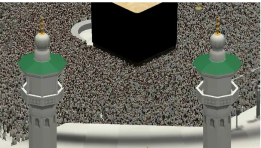
More complex desired behavior can be specified using navigation fields (Patil et al., 2011). These are spatially varying flow fields that define a desired velocity for an individual that depends on that individual’s position. Navigation fields can be used to specify desired overall flow patterns. For example, Figure 1.1 shows a still from the simulation of the Tawaf ritual, a part of the Islamic pilgrimage to Mecca for the Hajj. A navigation field is used to specify the desired counterclockwise motion pattern around the Kabah (central black structure) that is part of the ritual (for example see the simulations in (Schneider et al., 2011; Curtis et al., 2011)).
Figure 1.1: Still from a visualization of a simulation of the Tawaf ritual. Agents receive a desired velocity from a flow field directing them in a counterclockwise motion around the Kabah (central structure).
1.1.2 Computing Crowd Motion
Given the current state of the individuals in the crowd and the set of goals to reach, the crowd motion problem is to compute short-term paths which are responsive to the local conditions but still lead to an entity’s ultimate goals. Reynolds refers to the process of intermediate-level planning as steering behaviors. Steering behaviors in crowds are responsible for collision avoidance and local navigation, with the goal of making individuals in a crowd walk around each other in a natural manner (Reynolds, 1999).
This dissertation focuses on the problem of motion computation and steering behaviors for crowd simulation. More details on the approaches for motion planning in crowds are given in Section 1.2.
1.1.3 Animating and Rendering of Crowds
If the crowd simulation is to be used in a graphical environment, it is necessary to visually render the simulation results. Creating a natural visual rendering of the computed motion of human characters is a challenging but well-studied problem in computer graphics. The most standard approach for animating a human’s motion is known as a ‘walk cycle’, which involves translating the display of the human character’s center of mass along the motion vector while moving the character’s arms and legs in a simple, periodic cycle. The cyclic animation of limb motion can be either created by an artist or recorded from the motion of real humans using motion capture equipment.
The position of joint and limbs needed to produce natural walk cycles can be computed using Inverse Kinematics (IK) (Peiper, 1968). IK can be used to devise algorithms to dynamically adapt limb motion in order to create a variety of different types of walks, for example (Calvert et al., 1993) and (Bruderlin and Calvert, 1996). Recorded data of human motion can also be used to drive the motion of animated characters. For example, (Ko and Badler, 1993) provides a method of converting 2D rotoscoped data of human motion into walking animation appropriate for people moving at different speeds and for people of different genders, weights, and body types. Data-driven methods for animated characters have been extended into 3D as well (Witkin and Popovic, 1995), and can be used to synthesize a large variety of different recorded motions (Kovar et al., 2002).
be used in an aggressive fashion by using very simple geometry such as a single quad with a detailed human texture as described in (Tecchia et al., 2002), a technique known as impostors. Impostors can be combined with a geometric level of detail system to allow real-time rendering of thousands of agents as in (Dobbyn et al., 2005). Impostors can be improved by using more detailed, animated 2D geometry as is done in (Kavan et al., 2008). Using such methods can significantly reduce rendering costs, which is critical when creating real-time animation of crowds for interactive applications like games, training, and VR.
1.2 Motion in Crowds
Several methods can be employed to compute the motion of individuals in crowds. The choice of the most appropriate method depends on the type of crowds being simulated, the complexity of the environment, and the densities of the agents. The following subsections explain some of the high-level considerations that affect crowd simulation algorithms.
1.2.1 Heterogeneous Crowd Simulations
An important consideration in crowd simulation is whether the crowds being simulated are homogeneous or heterogeneous. The study of heterogeneous crowds date back to at least the work of Le Bon, who analyzed how members of a crowd can have different races, genders, intents, and backgrounds (Bon, 1895). This dissertation focuses on these types of heterogeneous crowds, where each individual maintains a distinct, observable identity. This identity may be seen in a person’s goals, desired speeds, politeness, cooperation, and many other factors affecting their motion.
homogeneity assumption found in this work has been relaxed by more recent approaches, such as (Treuille et al., 2006) which allows for a small, fixed number of goals, and (Narain et al., 2009) which allows for a unique goal for each individual in the crowd. However, these methods still enforce a continuum of motion, which results in nearby individuals being grouped together to share common characteristics and states such as similar speeds and motion, thereby reducing the heterogeneity of the simulation.
Agent-based Crowd Simulations:
In contrast to continuum methods, agent-based simulation methods allow for true heterogeneity in an individual’s motions. In these simulations, each person in the crowd is represented as a simulated agent (typically in a 1-to-1 correspondence). Since the motion of each agent can be computed independently, it is possible to simulate crowds with vastly differing motion for different agents, even those moving right next to each other.
An agent-based approach was taken in the Boids algorithm, the pioneering work of Reynolds (Reynolds, 1987). The Boids algorithm produced steering behavior that resembled flocking, herding, and school behaviors commonly observed in animal motion. Similar to Boids, this dissertation presents an agent-based model, but designed for simulation of human crowd motion.
1.2.2 Global Navigation
Computing an agent’s motion breaks down into two distinct tasks: local navigation and global navigation. Global navigation is the process of determining a long-term path that is free of local minima. To perform global navigation, it is common to use a spatial navigation data-structure, such as roadmaps, to guide agents around large, static obstacles in order to avoid local minima.
by a link if and only if the direct path between the two nodes is traversable (i.e. no obstacles block the direct path). Such roadmaps can be constructed by an artist, or automatically generated using visibility graphs (Lozano-P´erez and Wesley, 1979), probabilistic roadmaps (Kavraki et al., 1996), or other techniques (Latombe, 1991; LaValle, 2006).
Agents can compute global paths using such roadmaps. An agent chooses the closest node to its current position as a start vertex, and the closest vertex to its goal position as an end vertex. Paths can then be represented by a set of edges between vertices. To find the shortest path between the start and end vertex, standard graph search techniques, such as Dijkstra’s algorithm (Dijkstra, 1959) or A* (Hart et al., 1968), can be used. The direction along the current link towards the next vertex in the path forms a basis for an agent’sgoal velocity. It is the responsibility of the local navigation algorithm to move towards the goal velocity without colliding into other nearby agents.
1.2.3 Velocity Space Planning for Local Navigation
There are a variety of ways to perform local navigation and collision avoidance. A common technique is to plan based on the current positions of other nearby agents, with closer agents being given a greater weight when planning than farther away agents (for example by using repulsive forces which are inversely proportional to a neighbors distance). This technique is commonly used in simulations, including work by (Reynolds, 1987), (Helbing and Molnar, 1995), and (Pelechano et al., 2007).
These techniques implicitly assume that all of an agent’s neighbors will remain in the same position for the foreseeable future. As such, it is common for such methods to result in collisions between agents when traveling at high speeds and in complex cross-flows. Additionally, as agents come towards each other, forces typically grow exponentially, which can lead to issues with simulation stability and result in unnatural and oscillatory motion.
neighboring agent will constrain an agent’s potential velocities based on its relative positions and velocities. Planning in velocity space corresponds to making a short-term constant velocity assumption. This assumption allows for better avoidance behavior in complex, congested scenarios with lots of cross flows. See (Fiorini and Shiller, 1998) for a further discussion of velocity space planning.
Chapter 2 discusses how to adapt velocity space planning to scenarios where multiple agents simultaneously avoid each other. It also presents an efficient implementation of a velocity space planning technique designed to exploit the hardware trends discussed in Section 1.3.
1.3 Modern Processor Architecture Trends
There are various applications of crowd simulations where strong computational performance is important. For example, in computer games and related areas such as training and VR, crowds often must respond interactively to the actions of a user. This requirement means that the actions of all the agents in the crowd must be computed in a few milliseconds or less to reach the common simulation update target of 30Hz. Another example is architectural crowd flow analysis, where crowd simulations are used to predict crowd flows in new architectural or urban domains and to analyze which changes improve these flows. Architectural analysis benefits from exploring as many options as possible, as quickly as possible. When designing new simulation algorithms where computational performance is a major issue, it is important to look at the current trends in modern processors and understand how to exploit them.
increase in performance of single-core processing has slowed considerably in recent years due to power requirements (Borkar and Chien, 2011). Instead, growth in performance comes from larger vector processors (data-level parallelism) and more cores per chip (thread-level parallelism). Unlike ILP, exploiting these types of parallelism requires careful thought from an algorithm designer. In this dissertation, I develop algorithms that can utilize these increasing levels of parallelism to accelerate crowd simulation.
Another important trend in modern processors is the fact that the growth in compute power is outpacing the growth in cache speeds and memory access times. The result of this trend is to effectively reduce the cost of compute relative to each memory access. These architectural developments have a two-fold impact on the simulation algorithm. Firstly, because memory access is more likely to be a computation bottleneck, more compute-intensive approaches to crowd simulation can run at very similar speeds as other simpler, memory-access-bound methods. Secondly, it creates a greater importance for developing data-structures that can efficiently exploit the cache and other features of the memory subsystem in order to reduce the effect of memory access times. Together, these trends guide the development of the algorithms I present in this dissertation.
1.4 Thesis statement
My thesis is as follows:
1.5 Main Results
In support of my thesis statement, I present several results relating to generating effi-cient, large-scale, realistic crowd simulations. By using geometric optimization approaches I develop simulation techniques that are scalable, with applications from modeling the motion of just two people crossing paths to crowds of hundreds of thousands of people. To this end there are three main contributions. First, I demonstrate how to exploit the architecture of modern computer processors to efficiently compute these geometric optimization problems (Section 1.5.1). Second, I discuss how to incorporate important biomechanically inspired considerations into the optimization framework to produce more realistic simulations (Sec-tion 1.5.2). Third, I provide a method for simulating the effect of various personalities on a person’s path (Section 1.5.3). Additionally, I validate the motion predicted by this model against data of real humans paths to analyze the correctness of the proposed models (Section 1.5.4).
1.5.1 Parallel, Optimization-Based Collision Avoidance
One important result from this dissertation is a new technique for distributed collision avoidance. I present the ClearPath algorithm, an adaptation of velocity-based collision avoidance methods from robotics to the domain of distributed collision avoidance for crowd simulations.
Additionally, I discuss how the implementation of ClearPath exploits recent hardware trends to maximize performance. This performance improvement comes from increasing parallel processing, exploiting SIMD/vector processing, and using spatial data structures to reduce memory access costs.
(a) Bi-directional Flow (b) Dense Congestion (c) Evacuation
Figure 1.2: ClearPath performing collision avoidance on several large-scale scenarios with hundreds of agents at varying densities.
in the presence of obstacles, see Figure 1.2 for examples. These results were published in (Guy et al., 2009) and are discussed in Chapter 2.
1.5.2 Crowd Simulation based on the Principle of Least Effort
Additionally, in this dissertation I present a simulation algorithm that builds on distributed collision techniques, like ClearPath, to create biomechanically inspired crowd trajectories based on the Principle of Least Effort (PLE). The main result of this work is a unified framework for simulating crowds that reproduces several emergent phenomena commonly found in real crowds, and that matches real-world trajectory data from human crowds.
To understand the accuracy of these PLE-based simulations, I present several forms of analysis and comparison between the simulated trajectories and the known motion from actual human paths. I demonstrate that well-known emergent behaviors such as lane-formation and arching arise in both real human crowds and in these simulations, in both simple targeted set-ups and in simulations of complex real-world scenarios as shown in Figure 1.3. These results were published in (Guy et al., 2010a) and are discussed in Chapter 3.
(a) Narrow Passage (b) Shibuya Crossing (c) Long Corridor
Figure 1.3: Images of various crowd simulations using ideas inspired by biomechanics research. The simulations show a variety of emergent phenomena such as lane formation.
simulated aggregate flow rates in larger scenarios. These results were published in (Guy et al., 2012) and are discussed in Chapter 4.
1.5.3 Data Use in Crowd Modeling
I also present results related to incorporating various data into crowd simulations. Due to the complexity of human behavior, no model that simply tries to create rules from first principles can easily capture all aspects and variety of human motion as part of a crowd. Because of this variation, it can be necessary to use data of real crowds to guide simulations. I present a method for matching simulations closely to real world data. These results were published in (Guy et al., 2010b) and are discussed in Chapter 5.
I also present a method based on data from user-studies to simulate the diversity of behaviors that comes from different personalities. The result is a method that is able to simulate individuals with different apparent personalities such as “aggressive” or “shy”. These results were published in (Guy et al., 2011) and are discussed in Chapter 6.
1.5.4 Simulation Validation form Real-World Data
(a) Varying Personalities (b) Narrow Hallway (c) Street Crossing
Figure 1.4: (a) Data-driven crowd simulations (b-c) Data-driven evaluation scenarios
to validation data. Such a metric can ultimately be used to measure the accuracy of different simulation techniques, including those presented in this dissertation, at capturing different recorded crowd behaviors such as those seen in Figure 1.4b-c. These results are discussed in Chapter 7.
1.6 Organization
The rest of this dissertation is organized as follows: Chapter 2 presents the ClearPath algorithm for local navigation and provides a parallel implementation of the approach. This chapter also briefly discusses the Optimal Reciprocal Collision Avoidance (ORCA) collision-avoidance approach used later in the subsequent work.
Chapter 3 describes an algorithm for incorporating a biomechanically motivated version of the Principle of Least Effort into a distributed collision avoidance technique in order to create simulations of human crowds. Chapter 4 compares the motion computed by Least-Effort crowd simulations to the motion and flow of human crowds based on standard techniques used by pedestrian analysis and fire-safety researchers.
CHAPTER 2
ClearPath: A Method for Decentralized Collision Avoidance
2.1 Introduction
From record-setting crowds at rallies and protests to futuristic swarms of robots, our world is currently experiencing a continuing rise of complex, distributed collections of independently acting entities. All of these domains can be effective model as multi-agent system, that is as a set of interacting dynamic entities. With potential applications such as predicting crowd disasters, improving robot cooperation, and enabling the next generation of air travel, developing models to reproduce, control, predict and understand these types of systems is becoming critically important.
One of the key challenges in the area of multi-agent systems is to provide a means of producing and controlling the behaviors of the agents in the system, while maintaing important safety constraints. The work presented in this chapter focuses on maintaining collision-free motion while allowing each agent to reach it’s own (externally specified) goal. This approach will provide a decentralized solution where each agent can make it’s own navigation decisions without explicit communications with it’s neighbors nor a central authority.
One of the goals of this work is to study the computational issues involved in enabling real-time agent-based simulation to exploit current architectural trends. Recent and future commodity processors are becoming increasingly parallel. Specifically, current GPUs and upcoming x86-based many-core processors such as the experimental Larrabee processors consist of tens or hundreds of cores, with each core capable of executing multiple threads and vector instructions to achieve higher parallel-code performance. Therefore, it is important to design collision avoidance and simulation algorithms such that they can exploit substantial amounts of fine-grained parallelism.
2.1.1 Main Results
This chapter describes an algorithm for distributed, multi-agent collision avoidance called ClearPath. The approach is based on the robotics concept ofvelocity obstacles(VO) that was introduced by Fiorini and Shiller (Fiorini and Shiller, 1998) for motion planning among dynamic obstacles. By using an efficient velocity-obstacle based formulation that can be combined with any underlying multi-agent simulation, the local collision avoidance computations can be reduced to solving a quadratic optimization problem that minimizes the change in underlying velocity of each agent subject to non-collision constraints
In describing ClearPath I will present several main results:
1. A scaleable, decentralized approach for multi-agent collision avoidance
2. A multi-threaded implementation with dynamic load balancing
3. A method for exploiting SIMD/vector processing units for increased computation
2.1.2 Organization
The result of this chapter is organized as follows. Section 2.2 provides a brief review of closely related work. Section 2.3 describes in detail the ClearPath approach for local collision avoidance. Section 2.4 details a method for parallel implementation exploiting both thread-level and data-level parallelism. Sections 2.5 and 2.6 describes a basic method for incorporating this local collision avoidance method to simulate crowds and analyzes the performance of the resulting system. In Section 2.7, I discuss the limitations of this method and some scope for future work.
2.2 Previous Work
Different techniques have been proposed to model behaviors of individual agents, groups and heterogeneous crowds. Excellent surveys have been recently published including (Thalmann et al., 2006) and (Pelechano et al., 2008a). These include methods to model local dynamics and generate emergent behaviors such as (Reynolds, 1987) and (Reynolds, 1999); psychological effects and cognitive models like the work of (Shao and Terzopoulos, 2005) and (Yu and Terzopoulos, 2007); and cellular automata models and hierarchical approaches (Schadschneider et al., 2011). In this section, I give a brief overview of related work in collision detection and avoidance.
2.2.1 Collision detection and path planning
The problem of computing collision-free motion for one or multiple robots among static or dynamic obstacles has been extensively studied in robot motion planning (LaValle, 2006). These include global algorithms based on randomized sampling, local planning techniques based on potential field methods, centralized and decentralized methods for multi-robot coordination, etc. In general, these methods are either too slow for interactive applications or may suffer from paths that get stuck at local minima.
2.2.2 Collision avoidance
Collision avoidance problems have been been studied in control theory, traffic simula-tion, robotics and crowd simulation. Optimization techniques for local collision detection have been proposed for a pair of objects, including separation or penetration distance com-putation between convex polytopes (Cameron, 1997; Lin, 1993) and local collision detection between convex or non-strictly convex polyhedra with continuous velocities (Faverjon and Tournassoud, 1987; Kanehiro et al., 2008).
Different techniques have been proposed for collision avoidance in group andcrowd simulations for example (Reynolds, 1999), (Foudil and Noureddine, 2027),(Sugiyama et al., 2001), (Musse and Thalmann, 1997), (Thalmann et al., 2006), (Helbing et al., 2005),(Lamarche and Donikian, 2004), and (Sud et al., 2007b). These techniques can be based on local coordination schemes, velocity models, prioritization rules, force-based techniques, or adaptive roadmaps. Other techniques have used LOD techniques to trade-off fidelity for speed such as (Yersin et al., 2008).
also been proposed. However, these techniques provide higher-order path-planning with implementations that are not yet fast enough for very large simulations.
2.2.3 Parallel algorithms
Many parallel algorithms have been designed for collision detection, Voronoi diagrams and related geometric computations that can exploit multiple cores or vector capabilities of GPUs (Owens et al., 2007). Sud et al. (Sud et al., 2007a) use GPU-based discretized Voronoi diagrams for collision detection among scenes with few hundred agents. There is extensive literature on developing parallel and distributed algorithms for multi-agent simulations (Tolwinski, 2002) including work on specialized hardware such as the cell processor (Reynolds, 2006).
2.3 Local Collision Avoidance
This sections presents the mathematical details of the ClearPath collision avoidance algorithm. The resulting approach is general and can be combined with different crowd and multi-agent simulation techniques.
Assumptions and Notation: ClearPath assumes that the scene consists of heteroge-neous agents with static and dynamic obstacles. The behavior of each agent is governed by some extrinsic and intrinsic parameters and computed in a distributed manner for each agent independently. The overall simulation proceeds in discrete time steps and the state of each agent, including its position and velocity, is updated each time step. Given the position and velocities of all the agents at a particular time instantT, and a discrete time interval of T, the goal is to compute a velocity (and therefore a linear path) for each agent that results in no collisions during the interval[T, T + T]. This velocity will be recomputed for every
agent, every time step.
At any time instance, each agent has the information about the position and velocity of nearby agents. This can be achieved efficiently, but storing the position of every agent in a kD-tree, neighbors searches can then be preformed inO(log n) times. Each agent is represented using a circle or convex polygon in the plane. If the actual shape of the agent is non-convex, its convex hull can be used. The resulting collision-avoidance algorithm becomes conservative in such cases. In the rest of the chapter, a circular agent will be assumed, though the algorithm can be easily extended to other convex shapes.
Given an agentA,pA,rA, andvAis used to denote the agent’s position, radius and velocity, respectively. The algorithm assumes that the underlying simulation algorithm uses intrinsic and extrinsic characteristics of the agent or some high level model to compute desired velocity for each agent (vdes
A ) during the timestep. The symbolsvmax and amax will represent the maximum velocity and acceleration, respectively, of the agent during a timestep. Furthermore,q?denotes a line perpendicular to lineq.
2.3.1 Velocity Obstacles
ClearPath builds on the concept of velocity obstacles (Fiorini and Shiller, 1998). Let
A B represent the Minkowski sum of two objectsAandB and let Adenote the object Areflected in its reference point. Furthermore, let (p,v)denote the a ray starting atpand
heading in the direction ofv: (p,v) = {p+tv|t 0}.
LetAbe an agent moving in the plane andBbe a (moving) obstacle on the same plane. The velocity obstacleV OA
B(vB)of obstacleB to agentAis defined as the set consisting of all those velocitiesvAforAthat will result in a collision at some moment in time(t T) with obstacleB moving at velocityvB. This can be expressed as:
V OA
B(vB) =vA| (pA,vA vB)\B A6=;
This region has the geometric shape of a cone. Let (v,p, µ)denote the distance of
(v,p, µ) ={(v p)·µ}
Henceforth, the region inside the cone is represented as
V OAB(v) = ( (v,vB,p?AB lef t) 0)^( (v,vB,p?AB right) 0),
wherep?
AB lef t andp?AB right are the inwards directed rays perpendicular to theleftandright edges of the cone, respectively. The VO is a cone with its apex atvB(Fig. 2.1).
1233
45
1
63
–2
3
/ 2 Inside Segment Outside Segment Inside Point Outside Point Desired Velocity Computed Velocity LFVO
RFVO
TFVO
Figure 2.1: The Velocity ObstacleV OA
B(vB)of a disc-shaped obstacleB to a disc-shaped agentA. This VO represents the velocities that could result in a collision ofAwithB (i.e. potentially colliding region).
Van den Berg et al. (van den Berg et al., 2008a) presented an extension to VO called RVO. The resulting velocity computation algorithm guarantees an oscillation-free behavior for two agents. An RVO is formulated by moving the apex of the VO cone from vB to
(vA+vB)
2 . IfAhasN nearby neighbors, thenN avoidance cones will be created, and each agent needs to ensure that its desired velocity for the next frame,vdes
A , isoutsidethe union of allN velocity obstacle cones to avoid collisions. RVO algorithm performs random sampling of the 2D space in the vicinity of vdes
asN increases. In practice, RVO formulation can become overly conservative for tightly packed scenarios.
2.3.2 Optimization Formulation for Collision Avoidance
The local collision avoidance problem forN agents as a combinatorial optimization problem. ClearPath extends the VO formulation by imposing additional constraints that can guarantee collision avoidance for each agent during a given interval. It accounts for this time interval by defining a truncated cone to represent the collision-free region during the time interval corresponding to T. This finite time horizon velocity obstacle is denoted as FVO in this chapter. This truncation is a similar ideas presented in (Fiorini and Shiller, 1998), however here it is extend from one agent moving through unresponsive dynamic obstacles, to handle several responsive agents moving around each other. The original VO or RVO is defined using only two constraints (left and right), as shown in Fig. 2.1. The FVO is defined using a total of three conditions. Thetwoboundary cone constraints of the FVO are same as that of RVO:
FVOLA
B(v) = (v,(vA+vB)/2,p?AB lef t) 0 FVORA
B(v) = (v,(vA+vB)/2,p?AB right) 0
1233
45
1
63
–2
3
/ 2 Inside Segment Outside Segment Inside Point Outside Point Desired Velocity Computed Velocity L FVO R FVO T FVOFigure 2.2: The Finite-time horizon Velocity Obstacle FVOA
Ann additionally boundary is used to form an FVO:
Collision avoidance in only guaranteed for the duration T. This leads to a finite subset of the RVO cone that corresponds to the forbidden velocities that could lead to collisions in T. The truncated cone (expressed as shaded region in Figure 2.2) is bounded by a curve AB(v)(derivation is given in Appendix A). Due to efficiency reasons, AB(v)is replaced with a conservative linear approximation AB(v). Note that this approximation is conservative in nature, and in practice, this increases the area of the truncated cone by a small amount. This constitutes the additional constraint, defined as: FVOTA
B(v) =
AB(v) =
⇣
M pd?
AB ⇥⌘, p?AB
⌘
,where
⌘ = tan
✓
sin 1 rA+rB
|pAB|
◆
⇥(|pAB| (rA+rB)),and
M = (|pAB| (rA+rB))⇥pdAB+
vA+vB
2
Any feasible solution to all of constraints, which are separately formulated for each agent, will guarantee collision avoidance. A new, constraint satisfying velocity for each agent (in a distributed manner) which minimizes the deviation fromvdes
A –the velocity desired by the underlying simulation algorithm.
LetB1,..,BN represent theN nearest neighbors of an agent A. The computation of a new velocity (vnew
A ) can be posed as the following optimization problem:
Minimizek(vnewA vdesA )k2such that:
) ( 1 new A A B L v
FVO ( )
1 new A A B R v
FVO 1( new)
A A B
T v
FVO
(~ ~ ~ ( 1( new)
A A B C v FVO ~
·
( (··
) ( N new A A B L vFVO ( )
N new A A B R v
FVO N( new)
A A B
T v
FVO
(~ ~ ~ ( N( new)
A A B C v FVO ~ ( (
Let the union of all the FVO from an agent’s neighbors be referred to its potentially colliding region (PCR), and the boundary segments of each neighbor’s FVO as collectively
the Boundary Edges (BE). BE consists of 3N boundary segments – 3 from each neighbor of
A. By exploiting the geometric nature of the problem it is to possible to derive the following lemma (proof in Appendix A):
Lemma 1: Ifvdes
A is inside PCR,vnewA must lie on the boundary segment of the FVO of one of the neighbors.
In many simulations, there are other constraints on the velocity of an agent. For example, kineodynamic constraints (LaValle, 2006), which impose certain bounds on the motion (e.g. maximum velocity or maximum acceleration). In case the optimal solution to the quadratic optimization problem doesn’t satisfy these bounds, the constraints can be relaxed by removing the furthest agent fromA, and recomputing the optimal solution by considering onlyN 1agents. This relaxation step is carried on until an optimal solution
satisfying all the constraints is obtained.
2.3.3 ClearPath Implementation
1233
45
1
63
–2
3
/ 2 Inside Segment Outside Segment Inside Point Outside Point Desired Velocity Computed Velocity LFVO
RFVO
TFVO
This mathematical optimization formulation can be used to design a fast algorithm to compute a collision-free velocity for each agent independently. Specifically, Lemma 1 can be exploited to compute all possible intersections of the boundary segments ofBE
with each other. Consider segmentX in Figure 2.3. Thekintersection points of the FVO region labeled asX1, .. ,Xk. Note that these points are stored in a sorted order of increasing distance from the corresponding end point (X0) of the segment. Each intersection point can be further classified as beingInsideorOutsideofPCR. After performing this classification, the subsegments between these points can also as beingInsideorOutsideof thePCR, based
on the following lemma (proof in Appendix A):
Lemma 2: The first subsegment along a segment is classified as Outside iff both its end points are tagged as Outside. Any other subsegment is classified as Outside iff both its end points are Outside, and the subsegment before it is Inside thePCR.
For example, bothX0andX1are tagged asOutside, and hence the subsegmentX0X1 is tagged asOutside. However, the subsegmentX1X2 is tagged asInsidesinceX0X1 is OutsidethePCR.
After classifying the subsegments ofBE,Outsidesubsegments are considered, the
one closest tovdes
A is returned as the new velocity. The ClearPath algorithm performs the following steps for each agent:
Step 0.Given an agent, query the kD-tree for the N nearest agents, and compute the FVO constraints to arrive atBE.
Step 1.Compute the normals of the each segment inBE.
Step 2. Compute the intersection points along each segment ofBE with the remaining
segments ofBE.
Step 3.Classify the intersection points asInsideorOutsideof thePCR.
Step 4.Sort the intersection points for each segment with increasing distance from its corresponding end point.
compute/maintain the closest point for theOutsidesubsegments.
Step 6. In case the resulting solution does not satisfy the kineodynamic or velocity constraints, relaxing the constraints by removing the FVO corresponding to the furthest neighbor, and repeat the algorithm with fewer agents.
ForM number of total intersections segments inBE, the runtime of the algorithm for a single agent is O(N(N +M)).
Collision Resolution: Due to initialization conditions, numerical precision errors, and approximations in implementation is still it possible to have collision between agents. In cases when agents are colliding, they should choose a new velocity that resolves the collision as quickly as possible. This results in an additional set of constraints in velocity space this can be conservatively approximated as a cone (Figure 2.4). In this case, the Potentially Colliding Region is the intersection between two circles. The first circle, P, is the set of maximal velocities reachable by an agent in a single time step (a circle of radius
amax⇥ T). The second circle, R, is the Minkowski difference of the two agents:B A. The region which lies in the 1st circle, but not the second is the set of velocities which escapes the collision in 1 time step. The region which lies in both circles are reachable velocities which fail to resolve the collision next time step. This area is conservatively approximated with a cone, which create an additional constraint for any agents that are colliding. These constraints are combined with the existing PCR from the neighboring agents. A colliding agent’s preferred velocity is set to0so that the smallest possible velocity
which resolves the collision is chosen. This will minimize oscillations due to collision resolution.
2.4 P-ClearPath: Parallel Collision Avoidance