A Closed Form Solution
The Harvard community has made this
article openly available.
Please share
how
this access benefits you. Your story matters
Citation Agarwal, Sumit, John D. Driscoll, and David I. Laibson. Forthcoming. Optimal mortgage refinancing: a closed form solution. Journal of Money, Credit, and Banking.
Citable link http://nrs.harvard.edu/urn-3:HUL.InstRepos:9918811
Terms of Use This article was downloaded from Harvard University’s DASH repository, and is made available under the terms and conditions applicable to Open Access Policy Articles, as set forth at http:// nrs.harvard.edu/urn-3:HUL.InstRepos:dash.current.terms-of-use#OAP
Electronic copy available at: http://ssrn.com/abstract=1010702 Sumit Agarwal
Federal Reserve Bank of Chicago
John C. Driscoll Federal Reserve Board
David I. Laibson∗
Harvard University and NBER March 17, 2008
∗We thank Michael Blank, Lauren Gaudino, Emir Kamenica, Nikolai Roussanov, Dan Tortorice,
Tim Murphy, Kenneth Weinstein and Eric Zwick for excellent research assistance. We are par-ticularly grateful to Fan Zhang who introduced us to Lambert’s W-function, which is needed to express our implicit solution for the refinancing differential as a closed form equation. We also thank Brent Ambrose, Ronel Elul, Xavier Gabaix, Bert Higgins, Erik Hurst, Michael LaCour-Little, Jim Papadonis, Sheridan Titman, David Weil, and participants at seminars at the NBER Summer Insti-tute and Johns Hopkins for helpful comments. Laibson acknowledges support from the NIA (P01 AG005842) and the NSF (0527516). Earlier versions of this paper with additional results circulated under the titles “When Should Borrowers Refinance Their Mortgages?” and “Mortgage Refinancing for Distracted Consumers.” The views expressed in this paper do not necessarily reflect the views of the Federal Reserve Board or the Federal Reserve Bank of Chicago.
Electronic copy available at: http://ssrn.com/abstract=1010702 Abstract:
We derive the first closed-form optimal refinancing rule: Refinance when the current mortgage interest rate falls below the original rate by at least
1
ψ[φ+W(−exp (−φ))].
In this formulaW(.) is the LambertW-function,
ψ= p 2 (ρ+λ) σ , φ= 1 +ψ(ρ+λ) κ/M (1−τ),
ρ is the real discount rate, λ is the expected real rate of exogenous mort-gage repayment, σ is the standard deviation of the mortgage rate, κ/M
is the ratio of the tax-adjusted refinancing cost and the remaining mort-gage value, andτ is the marginal tax rate. This expression is derived by solving a tractable class of refinancing problems. Our quantitative results closely match those reported by researchers using numerical methods. JEL classification: G11, G21.
1. Introduction
Households in the US hold $23 trillion in real estate assets.1 Almost all home buyers obtain mortgages and the total value of these mortgages is $10 trillion, exceeding the value of US government debt. Decisions about mortgage refinancing are among the most important decisions that households make.2
Borrowers refinance mortgages to change the size of their mortgage and/or to take advantage of lower borrowing rates. Many authors have calculated the opti-mal refinancing differential when the household is not motivated by equity extraction considerations: Dunn and McConnell (1981a, 1981b); Dunn and Spatt (2005); Hen-dershott and van Order (1987); Chen and Ling (1989); Follain, Scott and Yang (1992); Yang and Maris (1993); Stanton (1995); Longstaff(2004); Kalotay, Yang and Fabozzi (2004, 2007, forthcoming); and Deng and Quigley (2006). At the optimal differential, the NPV of the interest saved equals the sum of refinancing costs and the difference between an old ‘in the money’ refinancing option that is given up and a new ‘out of the money’ refinancing option that is acquired.
The actual behavior of mortgage holders often differs from the predictions of the optimal refinancing model. In the 1980s and 1990s — when mortgage interests rates generally fell — many borrowers failed to refinance despite holding options that were deeply in the money (Giliberto and Thibodeau, 1989, Green and LaCour-Little (1999) and Deng and Quigley, 2006). On the other hand, Chang and Yavas (2006) have noted that over one-third of the borrowers refinancedtoo early during the period
1Flow of Funds Accounts of the United States, Board of Governors of the Federal Reserve System,
June, 2007.
2Dickinson and Heuson (1994) and Kau and Keenan (1995) provide extensive surveys of the
refinancing literature. See Campbell (2006) for a broader discussion of the importance of studying mortgage decisions by households.
1996-2003.3
Anomalous refinancing behavior may be partially due to the complexity of the problem. Previous academic research has derived the optimal differential as the implicit numerical solution of a system of partial differential equations. Such option-value problems may be difficult to understand for many borrowers and their advisers. For instance, in this paper we analyze a sample of leading sources of financial advice andfind that none of these books and web sites acknowledge or discuss the (option) value of waiting for interest rates to fall further. Instead these advisory services discuss a “break-even” net present value rule: only refinance if the present value of the interest savings is greater than or equal to the closing cost.
In the current paper, we derive a closed-form optimal refinancing rule. We be-gin our analysis by identifying an analytically tractable class of mortgage refinancing problems. We assume that the real mortgage interest rate and inflation follow Brown-ian motion, and the mortgage is structured so that its real value remains constant until an endogenous refinancing event or an exogenous Poisson repayment event. The Poisson parameter can be calibrated to capture the combined effects of moving events, principal repayment, and inflation-driven depreciation of the mortgage obligation.
The optimal refinancing solution depends on the discount factor, closing costs, mortgage size, the marginal tax rate, the standard deviation of the innovation in the mortgage interest rate, and the Poisson rate of exogenous real repayment. For calibrated choices of these parameters, the optimal refinancing differentials we derive
3Many other papers document and attempt to explain the puzzling behavior of mortgage
hold-ers, including: Green and Shoven, (1986); Schwartz and Torous (1989,1992, 1993); Giliberto and Thibodeau, (1989); Richard and Roll, (1989); Archer and Ling (1993); Stanton (1995); Archer, Ling and McGill (1996); Hakim (1997); LaCour-Little (1999); Bennett, Peach and Peristiani (2000, 2001); Hurst (1999); Downing, Stanton and Wallace (2001); and Hurst and Stafford (2004).
range typically from 100 to 200 basis points. We compare our interest rate differen-tials with those computed numerically by Chen and Ling (1989), who do not make many of our simplifying assumptions. We find that the two approaches generate recommendations that differ by fewer than 10 basis points.
We provide two analytic solutions: a closed form exact solution — which appears in the abstract — and a closed form second-order approximation, which we refer to as the square root rule. The closed form exact solution can be implemented on a calculator that can make calls to Lambert’s W-function (a little-known but easily computable function that has only been actively studied in the past 20 years). By contrast, our square root rule can be implemented with any hand-held calculator. The square root rule lies within 10 to 30 basis points of the exact solution.
As described above, other authors have alreadynumerically solved mortgage refi-nancing problems. Our contribution is to derive aclosed form solution. Our closed form solution has the disadvantage that we need to make several simplifying assump-tions that reduce the realism of the problem. Most importantly, our model studies optimal refinancing for risk neutral agents.
On the other hand, our closed form solution has several advantages. Our solution is transparent, tractable, and quickly verifiable — it is not a numerical black box. It reveals the parametric and functional properties of an optimal refinancing policy. It can be integrated into analytic models and it can be used for pedagogy. It plays the role of other simplifying frameworks in economics (analogous to linearization or higher-order Taylor expansions). Finally, it can be used by households or advisers who are making personalfinance decisions. Our square root rule is particularly easy to implement.
The paper has the following organization. Section 2 describes and solves the mort-gage refinancing problem. Section 3 analyzes our refinancing result quantitatively and compares our results to the quantitativefindings of other researchers. Section 4 doc-uments the advice of financial planners, and derives the welfare loss from following the net present value rule. Section 5 more generally discusses the value of having a closed-form solution and concludes.
2. The Model
In this section, we present a tractable continuous-time model of mortgage refinancing. The first subsection introduces the assumptions and notation. The next subsection summarizes the argument of the proof and reports the key results.
2.1. Notation and key assumptions.
The real interest rate and the inflation rate. We assume that the real interest rate, r, and inflation rate,π, jointly follow Brownian motion. Formally,
dr = σrdzr (1)
dπ = σπdzπ, (2)
wheredz represents Brownian increments, and cov(dr, dπ) =σrπdt. Hence the
nom-inal interest rate, i = r+π follows a continuous-time random walk. The random walk assumption is less tenable during times when interest rates are near the bounds of their historic ranges, as is presently true in the case of the United States. How-ever, current Japanese mortgage rates are over 3 percentage points lower than U.S. rates, suggesting that it is in principle possible for U.S. rates to fall from current
levels. More generally, in recent years global long-term interest rates have seemed less responsive to variations in short-term policy interest rates, which suggests that mean-reverting behavior in policy rates may not translate into mean-reverting behav-ior in long-term rates.4 Li, Pearson, and Poteshman (2004) argue that the nominal
interest rate is well-approximated by a random walk, and that estimates showing mean reversion are biased becaused of failure to condition on observed minimums and maximums.5
Nevertheless, the random walk approximation is controversial. Chen and Ling (1989), Follain, Scott and Yang (1992) and Yang and Maris (1993) assume that the nominal interest rate follows a random walk. However, other authors assume that interest rates are mean reverting (e.g. Stanton, 1995 and Downing, Stanton, and Wallace, 2005). We adopt the random walk assumption because it allows us to considerably simplify the analysis.
The interest rate on a mortgage is fixed at the time the mortgage is issued. Our analysis focuses on the gap between the current nominal interest rate, i=r+π,and the “mortgage rate,” i0 =r0+π0, which is the nominal interest rate at the time the
mortgage was issued. Let x represent the difference between the current nominal interest rate and the mortgage rate: x≡i−i0. This implies that
dx = pσ2
r+σ2π+ 2σrπdz (3)
= σdz, (4)
4This phenomenon was dubbed a conundrum by Greenspan (2005); Bernanke (2005) proposed a
“global savings glut” as a potential explanation for the low level of long-term interest rates.
5See Hamilton (1994) for a general discussion of the difficulties of distinguishing unit-root and
where σ ≡pσ2
r+σ2π + 2σrπ.
The mortgage contract. To eliminate a state variable, we counterfactually assume that mortgage payments are structured so that the real value of the mort-gage, M, remains fixed until an exogenous and discrete mortgage repayment event. These repayment events follow a Poisson arrival process. Excluding these discrete repayment events, the continuousflow of real mortgage repayment is given by
real flow of mortgage payments = (r0 +π0−π)M (5)
= (i0 −π)M. (6)
In a standard mortgage contract, thereal value of a mortgage obligation declines for three different reasons: repayment of the entire principal at the time of a relocation (or death), contracted nominal principal repayments, and inflationary depreciation of the real value of the mortgage. We capture all of these effects when we calibrate the exogenous arrival rate of a mortgage repayment event.
We assume that the mortgage is exogenously repaid with hazard rate λ. In our calibration section, we show how to choose a value of λ that simultaneously captures all three channels of repayment: relocation, nominal principal repayment, and inflation. Henceλshould be thought of as theexpected exogenous rate of decline in the real value of the mortgage.
Refinancing. The mortgage holder can refinance his or her mortgage at real (tax-adjusted) costκ(M). These costs include points and any other explicit or implicit transactions costs (e.g. lawyers fees, mortgage insurance, personal time). We define
deductions generated by future deductions of amortized refinancing points. For a consumer who itemizes (and takes account of all allowable deductions), the formula for κ(M)is provided in appendix A.6
Our analysis translates costs and benefits into units of “discounted dollars of in-terest payments.” Sinceκ(M)represents the tax-adjusted net present value of closing costs, κ(M) needs to be adjusted so that the model recognizes that one unit of κ is economically equal to 1−1τ dollars of current (fully and immediately tax-deductible) interest payments, where τ is the marginal tax rate of the household. Hence, we multiplyκ(M) by 1
1−τ and work with the normalized refinancing cost
C(M) = κ(M) 1−τ.
If a consumer does not itemize, set τ = 0 for both the calculation of κ(M) and the calculation of C(M).
Optimization problem. Mortgage holders pick the refinancing policy that minimizes the expected NPV of their real interest payments, applying a fixed dis-count rate, ρ. We also assume that mortgage holders are risk neutral.
Summing up these considerations, the consumer minimizes the expected value of her real mortgage payments. Let value function V(r0, r, π0, π, M), represent the
expected value of her real mortgage payments. More formally, the instantanteous
6A borrower who itemizes is allowed to make the following deduction. IfN is the term of the
mortgage, then the borrower can deduct 1
N of the points paid for N years. If the mortgage is
refinanced or otherwise prepaid, the borrower may deduct the remainder of the points at that time. Appendix A derives a formula forκ(M).
Bellman Equation for this problem is given by ρV = (r0+π0−π)M +λM −λV + E[dV] dt = (r0+π0−π+λ)M −λV + σ2r 2 ∂2V ∂r2 + σ2π 2 ∂2V ∂π2 +σrπ ∂2V ∂r∂π.
This Bellman equation can be derived with a standard application of stochas-tic calculus and Ito’s Lemma. First-order partial derivatives do not appear in this expression, sincer andπ have no drift.
At an endogenous refinancing event, the mortgage holder exchangesV(r0, r, π0, π, M)
for V(r, r, π, π, M) +C(M). Hence, at an optimal refinancing event value matching will imply that
V(r0, r, π0, π, M) =V(r, r, π, π, M) +C(M).
Given our assumptions, an optimizing mortgage holder picks a refinancing rule that minimizes the discounted value of her mortgage payments. In other words, she picks a refinancing rule that minimizesV.
We next show that the second-order partial differential equation that characterizes
V can be simplified.
2.2. Our main result. Since M is a constant, we can partial M out of the problem. This leaves four state variables: r0, r, π0, π.
The first step in the proof decomposes the value function V(r0, r, π0, π). We
restriction that refinancing is disallowed. The Bellman Equation for Z is given by,
ρZ(r0, r, π0, π) = (r0+π0−π+λ)M −λZ(r0, r, π0, π) +
E[dZ]
dt .
It can be confirmed that the solution forZ is
Z(r0, r, π0, π) =
(r0+π0 −π+λ)M
ρ+λ . (7)
It follows thatZ can be reduced to a function of the state variable−x+r, which is equal to r0+π0−π.
We decompose V, by defining R as
R(r0, r, π0, π)≡Z(r0, r, π0, π)−V(r0, r, π0, π). (8)
The function R represents the option value of being able to refinance. R can be expressed as a function of one state variable:
x = i−i0
= r+π−r0−π0.
Lemma 1. Replication.
R(r0, r, π0, π) =R(r0+∆, r+∆, π0, π) (9)
=R(r0, r, π0+∆, π+∆) (10)
=R(r0, r+∆, π0+∆, π) (11)
Proof: Consider an agent in state (r0+∆, r+∆, π0, π).Let this agent replicate
the refinancing strategy of an agent in state (r0, r, π0, π). In other words, refinance
after every sequence of innovations in the Ito processes that would make the agent who started at(r0, r, π0, π)refinance. So the agent in state(r0+∆, r+∆, π0, π)will
generate refinancing choices valued at V(r0, r, π0, π) +∆ρ+λM. Hence,
V(r0+∆, r+∆, π0, π)≤V(r0, r, π0, π) + ∆M ρ+λ. Likewise, we have V(r0, r, π0, π)≤V(r0+∆, r+∆, π0, π)− ∆M ρ+λ.
Combining these two inequalities, and substituting equations (7) and (8), yields equa-tion 9. We now repeat this type of argument for other cases. By replicaequa-tion,
V(r0, r, π0+∆, π+∆) ≤ V(r0, r, π0, π)
Combining these two inequalities, we have equation 10. By replication, V(r0, r+∆, π0+∆, π) ≤ V(r0, r, π0, π) + ∆M ρ+λ V(r0, r, π0, π) ≤ V(r0+∆, r, π0, π+∆)− ∆M ρ+λ.
Before refinancing, the perturbed agent pays∆more (the inflation rate at which the perturbed agent borrowed isπ0+∆rather thanπ0). After refinancing, the perturbed
agent pays∆ more (the real interest rate at which the perturbed agent refinances is
r+∆rather than r). Combining the two inequalities, we have equation 11. ¤ The Lemma implies that these equalities hold everywhere in the state space:
∂R ∂r = ∂R ∂π =− ∂R ∂r0 =−∂R ∂π0 .
This in turn implies thatR(r0, r, π0, π)can be rewritten as R(x).
We will show that the solution of R can be expressed as a second-order ordinary differential equation with three unknowns: two constants in the differential equation and one free boundary. To solve for these three unknowns we need three boundary conditions. We will exploit a value matching constraint that links R the instant before refinancing at x=x∗ and the instant after refinancing (when x= 0).
R(x∗) =R(0)−C(M)− x
∗M
ρ+λ
We will also exploit smooth pasting at the refinancing boundary.
R0(x∗) =− M
Finally,limx→∞R(x) = 0,since the option value of refinancing vanishes as the interest differential gets arbitrarily large. See Lemma 5 in Appendix B for a derivation of thefirst two boundary conditions.
The following theorem characterizes the optimal threshold, x∗, and the value functions. The threshold rule is expressed in x, the difference between the current nominal interest rate,i, and the nominal interest rate of the mortgage, i0.
Theorem 2. Refinance when
i−i0 ≤x∗ ≡
1
ψ[φ+W(−exp (−φ))]. (12)
where W(.) is the LambertW-function,
ψ= p 2 (ρ+λ) σ , φ= 1 +ψ(ρ+λ) κ/M (1−τ).
Whenx > x∗ the value function is
V(r0, r, π0, π) =−Ke−ψx+ (i0−π+λ)M ρ+λ , (13) where K7 is given by K = M e ψx∗ ψ(ρ+λ). (14)
The option value of being able to refinance is Ke−ψx when x > x∗. 7K has an equivalent solution,K=−¡e−ψx∗
−1¢−1³x∗M
ρ+λ +C(M)
´ .
Proof: We can express V as
V(x, r) = (−x+r+λ)M
ρ+λ −R(x).
Using Ito’s Lemma, derive a continuous time Bellman Equation forV:
ρV = (−x+r)M+ σ
2
2 ·
∂2V
∂x2 +λ(M −V). (15)
Substituting forV yields
(ρ+λ) µ (−x+r+λ)M ρ+λ −R ¶ = (−x+r+λ)M− σ 2 2 R 00. This simplifes to (ρ+λ)R= σ 2 2 R 00. (16)
The original value function V has been eliminated from the analysis, as has the variable r. The option value R(x) has a solution of the form R(x) = Ke−ψx, with
exponent
ψ=
p
2(ρ+λ)
σ .
We pickψ >0 to satisfy the limiting boundary condition (limx∗→∞R(x∗) = 0). The
remaining two parameters, K andx∗,solve the system of equations derived from the value matching and smooth pasting conditions.
Ke−ψx∗ = K −C(M)− x
∗M
ρ+λ (17)
−ψKe−ψx∗ = − M
We use the smooth pasting condition to solve for K and substitute it back into the value matching condition. Hence,
K = 1 ψ M eψx∗ ρ+λ , (19) yielding 1 ψ M ρ+λ = 1 ψe ψx∗ M ρ+λ −C(M)− x∗M ρ+λ, (20)
Multiplying through by the inverse of the left hand side yields:
eψx∗−ψx∗ = 1 + C(M)
M ψ(ρ+λ) (21)
Setk= 1+C(MM )ψ(ρ+λ)in Lemma 6 (Appendix B) to yield the closed form expression for x∗ in the statement of the theorem.¤
The Lambert W function, which appears in the solution, is the inverse function of f(x) = xex. Hence, z = W(z)eW(z). Although its origins can be traced to
Johann Lambert and Leonhard Euler in the 18th century, the function has only been extensively studied in the past 20 years. It has since been shown to be useful in solving a wide variety of problems in applied mathematics, and is built into a number of common mathermatical programming packages, including Maple, Mathematica and Matlab. For more information on the function and its uses, see Corless, Gonnet, Hare, Jeffrey and Knuth (1996) and Hayes (2005).
We also study an additional threshold value at which the reduction in the NPV of future interest payments (assuming no more refinancing) is exactly offset by the cost of refinancing, C(M). We refer to this as the NPV break-even threshold.8
Definition 3. The NPV break-even threshold,xN P V, is defined as
−x
N P VM
ρ+λ =C(M). (22)
Intuitively, the NPV break-even threshold is the point at which the expected interest payments saved from an immediate andfinal refinancing, −xM
ρ+λ, exactly offset
the tax-adjusted cost of refinancing,C(M).
2.3. Second-order expansion. Our closed form (exact) solution for the optimal refinancing differential requires calls to the Lambert W-function. We also provide an alternative solution that can be implemented on a hand-held calculator that does not output the LambertW-function.
The proof of the main theorem derives an implicit solution for x∗ (equation 21), which can be written as
f(x∗) =eψx∗−ψx∗−1−ψ(ρ+λ)C(M)
M = 0
A second-order Taylor series approximation to f(x∗) at x∗ = 0 is given by:
f(x∗) ≈ f(0) +f0(0)x∗+ 1 2f 00(0)x∗2 = −ψ(ρ+λ)C(M) M + 0·x ∗+ 1 2ψ 2 x∗2
Setting this to zero and solving forx∗ (picking the negative root) yields an approxi-mation that we refer to as the square root rule,
to refinance, this differential represents a lower bound to the refinancing decision; they also note that calculating the option value is complicated.
x∗ ≈ −
r σκ
M(1−τ)
p
2 (ρ+λ).
We evaluate the practical accuracy of this approximation in the calibration section below.9 We also evaluate a third-order approximation, which is given by an implicit
cubic equation.10
3. Calibration
We begin by illustrating the model’s predictions for the optimal threshold value x∗. We numerically solve equation (12) — the exact solution of the optimal refinancing problem — with typical values of parametersρ, τ , κ(M),σ, andλ. Analytic derivatives of the threshold with respect to these parameters are provided in Appendix C. We also provide a web calculator11 which readers can use to evaluate any calibration of
interest.
For ourfirst illustrative analysis, we choose a 5% real discount rate,ρ= 0.05. We assume a 28% marginal tax rate,τ = 0.28.12 We assume transactions costs of 1 point
and $2000;κ(M)is given by the formula in Appendix A (e.g. κ(M) = 0.01M+2000if
9Not all of the limit properties of the second-order approximation match those of the exact
solution. In particular, as the standard deviation of the mortgage rate,σ, goes to zero, the second-order approximation also goes to zero, while the exact solution goes to the NPV threshold. Because of this, at low values ofσ, the NPV threshold is a better approximation to the optimal threshold than is the second-order approximation. Since the NPV threshold is also easily calculable, a better refinancing rule than simply using the second-order approximation alone is to refinance when
x <min ½ − q σC(MM)p2(ρ+λ),−(ρ+λ)C(MM) ¾ .
10Higher order approximations provide greater accuracy at the cost of greater computational
complexity. In our view, only the second-order approximation is of significant interest due to its ease of calculation.
11http://www.nber.org/mortgage-refinance-calculator
12In the 2007 tax code, the 28% marginal tax rate applies to jointfilings for households with joint
income between $128,500 and $195,850, and to filings for single households with income between $77,100 and $160,850.
τ = 0). Thefixed cost ($2000) reflects a range of fees including inspection costs, title insurance, lawyers fees, filing charges, and non-pecuniary costs like time.13 Using
historical data, we estimate that the annualized standard deviation of the mortgage interest rate is σ= 0.0109.14
Finally, we need to calibrateλ,the expected real repayment rate of the mortgage. We need to calculate the value ofλ that corresponds to arealistic mortgage contract — one in which there are three forms of repayment: first, a probability of exogenous repayment (due to a relocation); second, principal payments that reduce the real value of the mortgage; third, inflation that reduces the real value of the mortgage. Formally, consider a household with a mortgage with a contemporaneous real (annual) mortgage payment of p, remaining principle M, an original nominal interest rate of
i0, and aμhazard of relocation (implying that μ1 is the expected time until the next
move). We’ll consider an environment with current inflation π. For this mortgage, the expected (flow) value of the exogenous decline in the real mortgage obligation is
μM + (p−i0M) +πM.
The term in parentheses corresponds to contracted principal repayment. The last term represents inflation eroding the real value of the mortgage. Using this formula,
13See Federal Reserve Board and Office of Thrift Supervision (1996), Caplin, Freeman and Tracy
(1997), Danforth (1999), Lacour-Little (2000), and Chang and Yavas (2006) for data on transactions costs.
14The standard deviation for monthly differences of the Freddie Mac 30-year mortgage rate from
April 1971 to February 2004 is 0.00315, implying an annualized standard deviation of σ=√12× 0.00315 = 0.0109. By comparison, taking annual differences yields an average standard deviation of
we can calibrate the value of λ. λ = μ+³ p M −i0 ´ +π = μ+ µ pnominal Mnominal − i0 ¶ +π
In practice it will be easier for households to use the latter “nominal” version of the formula since households know pnominal and Mnominal, the nominal analogs of p and
M.15
We can also solve for the key terms in the equations above using formulae for a standardfixed rate mortgage. In this case, the calibration forλ is
λ=μ+ i0
exp [i0Γ]−1 +π.
where Γ is the remaining life (in years) of the mortgage. See Appendix D for this derivation.
Assume that the household has a 10% chance of moving per year, so μ= 10%,16
and the expected duration of staying the house is 10 years. Assume thati0 = 0.06,
π= 0.03, andΓ= 25 years, then,λ= 0.147.
Table 1 reports the optimal refinancing differentials calculated with our model for the calibration summarized above. We report the exact optimal rule, the second-and third-order approximations to the optimal rule, second-and the (suboptimal) net present value rule. We calculate the refinancing differentials for mortgage sizes (M) of
15This calibration is only an approximation, since the calibration formula will change over time
(whereasλis constant in the model from section 2).
16Hayre, Chaudhary and Young (2000) estimate that 5 to 7 percent of single-family homes turn
$1,000,000, $500,000, $250,000 and $100,000.
Table 1: Refinancing differentials in basis points by solution method
Mortgage Exact optimum 2nd order 3rd order NPV rule
$1,000,000 107 97 109 27
$500,000 118 106 121 33
$250,000 139 123 145 44
$100,000 193 163 211 76
The optimal refinancing threshold increases as mortgage size decreases, since in-terest savings from refinancing scale proportionately with mortgage size but part of the refinancing cost isfixed ($2000). The second-order approximation deviates by 10 to 30 basis points from the exact optimum. The third-order approximation deviates by only 2 to 18 basis points from the exact optimum. The NPV rule, by contrast, deviates by 80 to 117 basis points from the exact optimum.
Table 2 presents results for the six different marginal tax rates that were in effect under the tax code in 2006:
Table 2: Optimal refinancing differentials in basis points by marginal tax rate τ
τ Mortgage 0% 10% 15% 25% 28% 33% 35% $1,000,000 99 101 103 106 107 109 110 $500,000 108 111 113 117 118 121 122 $250,000 124 129 131 137 139 143 145 $100,000 166 174 178 189 193 199 202
The optimal differentials rise as the marginal tax rate rises, since interest payments are tax deductible but refinancing costs are not.
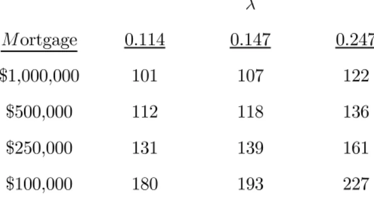
Table 3 reports the consequences of varying λ, the expected real rate of repay-ment.17 We consider cases in which the expected time to the next move is 5 years
(μ = 0.20), 10 years (μ = 0.10), and 15 years (μ = 0.066), corresponding to values for λ of .247, .147, and .114, respectively.
Table 3: Optimal refinancing differentials in basis points by expected real rate of repayment λ
λ Mortgage 0.114 0.147 0.247 $1,000,000 101 107 122 $500,000 112 118 136 $250,000 131 139 161 $100,000 180 193 227
As expected, a higher hazard rate of prepayment raises the optimal interest rate differential, since the effective amount of time over which the lower interest savings will be realized is smaller.
Table 4 reports the optimal differential assuming a refinancing cost of only $1000, which is of interest because of the wider availability of low-cost refinancings. For comparison, we also report the differentials predicted by the NPV rule at a refinancing cost of $1000.
17Unless otherwise specified, we now return to our earlier assumption of a marginal tax rate of
Table 4: Optimal refinancing differentials in basis points by fee size
C(M) Mortgage $2000 + 0.01M $1000 $1000, NPV $1,000,000 107 32 2 $500,000 118 45 4 $250,000 139 66 7 $100,000 193 108 18
Reducing the costs substantially reduces the optimal interest rate differentials. The differentials implied by the NPV rule also decline.
4. Comparison with Chen and Ling (1989)
We now compare the refinancing differentials implied by our model and those reported by Chen and Ling (1989). Chen and Ling calculate optimal differentials for a model in which the log one-period nominal interest rate follows a random walk, the time of exogenous prepayment (or the expected holding period) is known with certainty, and the real mortgage principle is allowed to decline over time because of inflation and continuous principle repayment. Chen and Ling use numerical methods to solve the resulting system of partial differential equations.
In contrast to their analysis, we make a simplifying assumption that allows us to obtain ananalytic solution to a closely related mortgage refinancing problem.18 As
explained above, we assume that the mortgage is structured so that its real value
18In one way, our paper adds greater realism when compared with previous work. We account
for the differential tax treatment of mortgage interest payments and refinancing costs. Refinancing costs are not tax deductible (unlike the closing costs on an originating mortgage).
remains constant. This allows us to avoid tracking a changing value of time to maturity and a changing remaining mortgage balance. In contrast to our approach, Chen and Ling’s model directly incoporates the effects of principal repayment and thefinite life of the mortgage contract.
To bring our model into line with theirs, our parameterλ is calibrated to capture the joint effects of moving, principal repayments, and inflation. Hence, λ is set to capture the three ways that the expected real value of the mortgage declines over time.
To calibrate our model to match the set-up in Chen and Ling, we set λ = 0.173
to account for (1) an 8 year expected holding period (1μ = 8, so μ = 0.125); (2) a long-run inflation forecast (in 1989) of 4% (π = 0.04); and (3) a principal repayment rate of 0.8% at the beginning of a 30-year mortgage. We set the discount rate to be 4%, ρ = 0.04, matching Chen and Ling’s assumption of an 8% nominal interest rate. Chen and Ling’s random walk assumption for the log short-term interest rate allows us to compute the implied standard deviation for the 30-year mortgage rate (see Appendix E). We calculate an implied standard deviation for the innovations of the 30-year mortgage rate of σ = 0.012. Finally, to match the analysis of Chen and Ling we assume a zero marginal tax rate.19
Chen and Ling’s baseline calculations exclude the possibility of subsequent refi-nancings. But their analysis enables us to compute the additional points that would be necessary to buy a new refinancing option when the original mortgage is refinanced. There are two such cases that are analyzed in Chen and Ling.
With a refinancing cost of 2 points (without a new option to refinance), 2.24
19We take results from the middle columns of their table 2. For consistency with our framework,
additional points are charged to purchase the right to refinance again,20 implying
total points of 4.24. For this case, Chen and Ling calculate an optimal refinancing differential of 228 basis points, while we calculate an optimal refinancing differential of 218 basis points, a difference of 10 basis points.
With a refinancing cost of 4 points (without a new option to refinance), 1.51 additional points will be charged to purchase the right to refinance again,21 implying
total points of 5.51 points. For this case, Chen and Ling calculate an optimal refinancing differential of 256 basis points, while we calculate an optimal differential of 255 basis points, a difference of 1 basis point.22
5. Financial advice
Households considering refinancing use many different sources of advice, including mortgage brokers, financial planners, financial advice books, and websites. In this section, we describe the refinancing rules recommended by 25 leading books and websites. We find that none of the sources of financial advice in our sample provide a calculation of the optimal refinancing differential. Instead, the advisory services in our sample offer the break-even NPV rule as the only theoretical benchmark. Most of the advice boils down to the following necessary condition for refinancing — only refinance if you can recoup the closing costs of refinancing in reduced interest payments.
First, we sampled books that were on top-ten sales lists at the Amazon and Barnes & Noble web sites (see the web appendix for a detailed description of our sampling
20See panel 1, column 3, in Table 1 of Chen and Ling. 21See panel 1, column 3, in Table 1 of Chen and Ling.
22The second order approximations yield refinancing differentials of 182 and 207, differing from
Chen and Ling’s values by 46 and 48 basis points. These results reflect the general deterioration of the approximation as refinancing costs become very large.
method andfindings23). Of the 15 unique books in our sample, 13 provided a
break-even calculation of some sort. Most of the 15 books also provided some rules of thumb (e.g. ‘wait for an interest differential of 200 basis points,’ or ‘only refinance if you can recoup the closing costs within 18 months’).
For websites, we entered the words mortgage refinancing advice into Google and examined the top twelve sites which offered information on refinancing. Two of these sites suggest a fixed interest-rate differential of one-and-a-half to two percent and recommend refinancing only if the borrower plans to stay in the house for at least three tofive years. One of the sites provides a monthly savings calculator, while seven of the sites provide a refinancing calculator based on the NPV break-even criterion. The remaining three sites did not provide a refinancing calculator but still recommend break-even calculations.
None of the 15 books and 10 web sites in our sample discuss (or quantitatively analyze) the value of waiting due to the possibility that interest rates might continue to decline.
Although our sampling procedure above did not identify books or websites that mentioned option value considerations, that does not mean that such sites do not exist. Indeed, there is at least one website that does implement a numerical op-tion value soluop-tion (http://www.kalotay.com; Kalotay, Yang and Fabozzi 2004, 2007, forthcoming).
Finally, market data also shows that many households did refinance too close to the NPV break-even rule during the last 15 years; see, for example, Yavas and Chang (2006) and Agarwal, Driscoll and Laibson (2004).
How suboptimal is the NPV rule?. To measure the suboptimality of the NPV rule, we consider an agent that starts life with state variablex= 0(a new mort-gage). We calculate the expected cost of using an arbitrary refinancing differential,
xH, instead of using theoptimal refinancing rule specified in Theorem 2.
Proposition 4. The expected discounted Loss as a fraction of the mortgage size from using an arbitrary heuristic rule instead of using the optimal rule is given by
Loss M = C(M) M + x∗ ρ+λ 1−e−ψx∗ − C(M) M + xH ρ+λ 1−e−ψxH (23) = e ψx∗ ψ(ρ+λ)− C(M) M + xH ρ+λ 1−e−ψxH . (24)
where xH is the heuristic threshold rule. This implies that the expected discounted Loss as a fraction of the mortgage size from using the suboptimal NPV rule instead of using the optimal rule is given by
Loss
M =
eψx∗
ψ(ρ+λ). (25)
Proof: The loss is equal to the difference between the value function associated with the optimal rule and the value function associated with the alternative rule. The value function for the optimal rule is given in the statement of the main theorem. Since the interest payment term is the same for both the optimal and suboptimal rules, the difference in value functions will be equal to the difference in option value expressions. For both the suboptimal and approximate rules, the value matching condition still applies, but withx∗ replaced with the suboptimal differentials specified by the alternative rule,xH.
Following the line of argument in the proof of our main theorem, the option value function, R(x), has a solution of the form R(x) = Ke−ψx. The parameter K is
derived from the value matching condition,
Ke−ψxH =K−C(M)− x HM ρ+λ, (26) implying K = C(M) + xHM ρ+λ 1−e−ψxH . (27)
So the difference in value functions is given by
Loss M = "C(M) M + x∗ ρ+λ 1−e−ψx∗ − C(M) M + xH ρ+λ 1−e−ψxH # e−ψx = " eψx∗ ψ(ρ+λ)− C(M) M + xH ρ+λ 1−e−ψxH # e−ψx.
Note thatxH =xN P V implies that C(M)
M + xH ρ+λ = 0, and hence Loss M = C(M) M + x∗ ρ+λ 1−e−ψx∗ e− ψx= eψ(x ∗−x) ψ(ρ+λ).
Setx= 0,to reflect the perspective of an agent with a newly issued mortgage. ¤ Note that the loss from following the NPV rule is equal to the option value of the ability to refinance, evaluated for a new mortgage. By ignoring the existence of the option value, the NPV rule creates a loss equal in size to the option value.
Using the same calibration assumptions that were used in section 3, we calculate the economic losses of using the NPV rule and the second order rule instead of the
exactly optimal rule.
Table 5: Expected losses in discounted dollars from using the NPV and approximate rules
Mortgage Loss (NPV rule) Loss (square root rule) $1,000,000 $163,235 $15,253
$500,000 $86,955 $9,459 $250,000 $49,066 $7,020 $100,000 $26,479 $6,406
Table 6: Expected losses as a percent of mortgage face value from using the NPV and approximate rules
Mortgage Loss (NPV rule) Loss (square root rule)
$1,000,000 16.3% 1.5%
$500,000 17.4% 1.9%
$250,000 19.6% 2.8%
$100,000 26.8% 6.4%
Other rules of thumb. Some advisers also refer to a rule of thumb in which borrowers are encouraged to refinance when the interest rate has dropped by 200 basis points. We have also heard more recently of a revised 100 basis point rule of thumb. Both rules generally, though not always, imply refinancings at bigger differentials than those implied by the NPV rule. However, our simulations show that the optimal refinancing differential can vary quite substantially by expected holding period and refinancing cost, among other parameters. Hence a “one sizefits all” rule will lead to substantial welfare losses.
6. Conclusion
Optimal mortgage refinancing rules have been calculated previously by numerically solving a system of partial differential equations. This paper derives the firstclosed form solution to a mortgage refinancing problem.
Our closed form solution has the disadvantage that we need to make several simpli-fying assumptions — e.g. risk neutrality. On the other hand, closed-form solutions are transparent, tractable, and easily verified — they are not a numerical black box. The functional contribution of each parameter to the solution is immediately apparent. One can easily make comparative statics calculations and can compute other impor-tant magnitudes — e.g. welfare calculations — without resorting to computational methods. Closed-form solutions are useful for pedagogy and as building blocks for more complex models. Analytic approximations are frequently used in the natural sciences and engineering to improve our understanding of ‘exact’ numerical models.24
Our derived refinancing rule takes the following form: Refinance when the current mortgage interest rate falls below the original mortgage interest rate by at least
1
ψ[φ+W(−exp (−φ))],
where W(.) is the LambertW-function,
ψ= p 2 (ρ+λ) σ , φ= 1 +ψ(ρ+λ) κ/M (1−τ),
24For example, Driscoll, Downar, and Pilat (1990) provide simple linear models useful in nuclear
reactor design. They argue that such models can help verify the output from black-box computer simulations.
ρ is the real discount rate, λ is the expected real rate of exogenous mortgage repay-ment (including the effects of moving, principal repayrepay-ment, and inflation), σ is the annual standard deviation of the mortgage rate, κ/M is the ratio of the tax-adjusted refinancing cost and the remaining value of the mortgage, and τ is the marginal tax rate.
All of these variables are easy to calibrate, including λ. This variable can be calibrated with the annual probability of relocating (μ), the ratio of total mortgage payments to the remaining value of the mortgage ³pn o m in a l
Mn o m in a l
´
, the initial mortgage interest rate (i0), and the current inflation rate (π):
λ=μ+ µ pnominal Mnominal − i0 ¶ +π.
Equivalently,λcan be calculated by using the remaining years left until the mortgage is fully repaid (Γ):
λ =μ+ i0
exp(i0Γ)−1+π.
We analyze both the exact solution of our mortgage refinancing problem (above) and a useful approximation to that solution. We show that a second-order Taylor expansion yields a square-root rule for optimal refinancing: Refinance when the current mortgage interest rate falls below the original mortgage interest rate by at
least s
σκ/M
(1−τ)
p
2 (ρ+λ).
Finally, we show that many leading sources of financial advice do not discuss (formally or informally) option value considerations. Advisory services typically discuss the net present value rule: refinance only if the net present value of the
interest saved is at least as great as the direct cost of refinancing. Compared to the optimal refinancing rule, the NPV rule generates expected discounted losses of over $85,000 on a $500,000 mortgage.
References
Agarwal, Sumit, John C. Driscoll and David I. Laibson (2004). “Mortgage Refi-nancing for Distracted Consumers.” Mimeo, Federal Reserve Bank of Chicago, Federal Reserve Board, and Harvard University.
Archer, Wayne and David Ling (1993). “Pricing Mortgage-Backed Securities: In-tegrating Optimal Call and Empirical Models of Prepayment.” Journal of the
American Real Estate and Urban Economics Association, 21(4), 373-404.
Bennett, Paul, Richard W. Peach, and Stavros Peristiani (2000). “Implied Mortgage Refinancing Thresholds,”Real Estate Economics, 28(3), 405-434.
Bennett, Paul, Richard W. Peach, and Stavros Peristiani (2001). “Structural Change in the Mortgage Market and the Propensity to Refinance,” Journal of Money,
Credit and Banking, 33(4), 955-975.
Bernanke, Ben S. (2005). “The Global Savings Glut and the U.S. Current Account Deficit.” Remarks at the Sandridge Lecture, Virginia Association of Economics, Richmond, Virginia, March 10.
Blanchard, Olivier J. and Nobuhiro Kiyotaki (1987). “Monopolistic Competition and the Effects of Aggregate Demand.” American Economic Review, 77(3), 647-666.
Campbell, John (2006). “Household Finance.”Journal of Finance, 56(4), 1553-1604. –— and Joao Cocco, 2001. “Household Risk Management and Optimal Mortgage
Choice.” Mimeo, Harvard University.
Caplin, Andrew, Charles Freeman and Joseph Tracy. “Collateral Damage: Refi-nancing Constraints and Regional Recessions.” Journal of Money, Credit and
Banking, 29(4), 497-516.
Chang, Yan and Abdullah Yavas (2006). “Do Borrowers Make Rational Choices on Points and Refinancing?” Mimeo, Freddie Mac.
Chen, Andrew and David Ling (1989). “Optimal Mortgage Refinancing with Sto-chastic Interest Rates,”AREUEA Journal, 17(3), 278-299.
Corless, R.M., G.H. Gonnet, D.E.G. Hare, D.J. Jeffrey and D.E. Knuth (1996). “On the Lambert W Function.” Advances in Computational Mathematics, 5, 329-359.
Danforth, David P. (1999). “Online Mortage Business Puts Consumers in Drivers’ Seat.”Secondary Mortgage Markets, 16(1), 2-8.
Deng, Yongheng, and John Quigley (2006). “Irrational Borrowers and the Pricing of Residential Mortgages,” Working Paper, University of California-Berkeley. Deng, Yongheng, John Quigley, and Robert van Order (2000). “Mortgage
Termi-nation, Heterogeneity and the Exercise of Mortgage Options,” Econometrica,
68(2), 275-307.
Dickinson, Amy and Andrea Hueson (1994). “Mortgage Prepayments: Past and Present,” Journal of Real Estate Literature,2(1), 11-33.
Dixit, Avinash and Joseph Stiglitz (1977).“Monopolistic Competition and Optimum Product Diversity.” American Economic Review, 67(2), 297-308.
Downing, Christopher, Richard Stanton and Nancy Wallace (2005). “An Empirical Test of a Two-Factor Mortgage Valuation Model: How Much Do House Prices Matter?” Real Estate Economics, 33(4), 681-710.
Driscoll, M.J., T. J. Downar and E. E. Pilat (1990). The Linear Reactivity Model
for Nuclear Fuel Management. American Nuclear Society, La Grange Park
Illinois.
Dunn, Kenneth B. and John McConnell (1981a). “A Comparison of Alternative Models of Pricing GNMA Mortgage-Backed Securities.” Journal of Finance,
36(2), 375-92.
Dunn, Kenneth B, and John McConnell (1981b). “Valuation of GNMA Mortgage-Backed Securities.”Journal of Finance, 36(3), 599-617.
Dunn, Kenneth B. and Chester S. Spatt (2005). “The Effect of Refinancing Costs and Market Imperfections on the Optimal Call Strategy and the Pricing of Debt Contracts.”Real Estate Economics, 33(4), 595-617.
Federal Reserve Board and Office of Thrift Supervision (1996). A Consumer’s Guide
to Mortgage Refinancing.
Follain, James R., Louis O. Scott and T.L. Tyler Yang (1992). “Microfoundations of a Mortgage Prepayment Function.”Journal of Real Estate Finance and
Eco-nomics, 5(1), 197-217.
Follain, James R. and Dan-Nein Tzang (1988). “The Interest Rate Differential and Refinancing a Home Mortgage.” The Appraisal Journal, 61(2), 243-251.
Gabaix, Xavier, Arvind Krishnamurthy and Olivier Vigneron (2007). “Limits of Ar-bitrage: Theory and Evidence from the Mortgage-Backed Securities Market.”
Journal of Finance, 62(2), pp. 557-595.
Gabaix, Xavier and David I. Laibson (2006). “Shrouded Attributes, Consumer My-opia, and Information Suppression in Competitive Markets.”Quarterly Journal
of Economics, 121(2), 505-540.
Giliberto, S. M., and T. G. Thibodeau, (1989). “Modeling Conventional Residential Mortgage Refinancing.” Journal of Real Estate Finance and Economics, 2(1), 285-299.
Green, Jerry, and John B. Shoven, (1986). “The Effects of Interest Rates on Mort-gage Prepayment,” Journal of Money, Credit, and Banking, 18(1), 41-59. Green, Richard K. and Michael LaCour-Little (1999). “Some Truths about
Os-triches: Who Doesn’t Prepay Their Mortgages and Why They Don’t.” Journal
of Housing Economics, 8(3), 233-248.
Greenspan, Alan (2005). Semiannual Monetary Policy Report to the Congress, February 16.
Hamilton, James D. (1994). Time Series Analysis. Princeton: Princeton Univer-sity Press.
Harding, J. P., (1997). “Estimating Borrower Mobility from Observed Prepayment.”
Real Estate Economics, 25(3), 347-371.
Hayes, Brian (2005). “Why W?” American Scientist, 93(2), 104-108.
Hayre, Lakhbir S., Sharad Chaudhary and Robert A. Young (2000). “Anatomy of Prepayments.” The Journal of Fixed Income, 10(1), 19-49.
Hendershott, Patrick and Robert van Order (1987). “Pricing Mortgages—An Inter-pretation of the Models and Results.” Journal of Financial Services Research, 1(1), 19-55.
Hurst, Erik (1999). “Household Consumption and Household Type: What Can We Learn from Mortgage Refinancing?” Mimeo, University of Chicago.
Hurst, Erik, and Frank Stafford (2004). “Home is Where the Equity is: Mort-gage Refinancing and Household Consumption.”Journal of Money, Credit, and
Kalotay, Andrew, Deane Yang and Frank J. Fabozzi (2004). “An Option-Theoretic Prepayment Model for Mortgages and Mortgage-Backed Securities.”
Interna-tional Journal of Theoretical and Applied Finance. 7(8), pp. 949-978.
–— (2007). “Refunding Efficiency: a generalized approach.” Applied Financial
Economics Letters, 3(3), pp. 141-146..
–— (forthcoming). “Optimal Refinancing: Bringing Professional Discipline to Household Finance.” Applied Financial Economics Letters.
Kau, James and Donald Keenan (1995). “An Overview of the Option-Theoretic Pricing of Mortgages.” Journal of Housing Research,6(2), 217-244.
LaCour-Little, Michael (1999). “Another Look at the Role of Borrower Characteris-tics in Predicting Mortgage Prepayments.”Journal of Housing Research,10(1), 45-60.
–— (2000). “The Evolving Role of Technology in Mortgage Finance.” Journal of
Housing Research, 11(2), 173-205.
Li, Minqiang, Neil D. Pearson and Allen M. Poteshman (2004). “Conditional Esti-mation of Diffusion Processes.”Journal of Financial Economics, 74(1), 31-66. Longstaff, Francis A. “Optimal Recursive Refinancing and the Valuation of
Mortgage-Backed Securities.” NBER Working Paper 10422.
Miller, Merton H. (1991). “Leverage.”The Journal of Finance, 46(2), 479-488 Quigley, John M. (1987). “Interest Rate Variations, Mortgage Prepayments and
Household Mobility.”The Review of Economic and Statistics, 69(4), 636-643. Richard, Scott F. and Richard Roll (1989). “Prepayments on Fixed-Rate
Mortgage-Backed Securities.”Journal of Portfolio Management, Spring, 73-82.
Schwartz, Eduardo S., and Walter N. Torous (1989). “Prepayment and the Valuation of Mortgage Pass-Through Securities.”Journal of Finance, 44(2), 375-392. Schwartz, Eduardo S., and Walter N. Torous (1992). “Prepayment, Default, and the
Valuation of Mortgage Pass-Through Securities.” Journal of Business, 65(2), 221-239.
Schwartz, Eduardo S., and Walter N. Torous, (1993). “Mortgage Prepayment and Default Decision: A Poisson Regression Approach,” Journal of the American
Stanton, Richard (1995). “Rational Prepayment and the Valuation of Mortgage-Backed Securities.”Review of Financial Studies, 8(3), 677-708.
–—, (1996). “Unobserved Heterogeneity and Rational Learning: Pool-Specific versus Generic Mortgage-Backed Security Prices.”Journal of Real Estate Finance and
Economics, 12(1), 243-263.
Tang, T.L. Tyler, and Brian A. Maris (1993). “Mortgage Refinancing with Asym-metric Information.”Journal of the American Real Estate and Urban Economics
Appendix A: Partial deductibiity of points
Let κ(M) = F +f M, where F denotes the fixed cost of refinancing and 100×f
is the number of points. The expected arrival rate of a full deductibility event — a move or a subsequent refinancing — is θ. At date t, the probability that such a full deductibility event has not yet occurred is e−θt. The likelihood that such an event
occurs at date t isθe−θt.
Assume the term of the new mortgage is for N years. Each year, borrowers are allowed to deduct amount f MN from their income, producing a tax reduction of τ f MN . At the time of a full deductibility event, borrowers immediately deduct all of the remaining undeducted points — i.e. they reduce their taxes by τ f M¡N−T
N
¢
.
The real value of the deduction declines at the rate of inflation. Hence, the payments are discounted effectively at the real discount rate r=ρ+π.
The present value of these tax benefits is then:
Z N 0 e−θte−(ρ+π)t µ τ f M N ¶ dt+ Z N 0 θe−θte−(ρ+π)t(τ f M) µ 1− t N ¶ dt.
Using integration by parts, this simplifies to
τ f M θ+ρ+π ∙µ 1−e−(θ+ρ+π)N N ¶ µ ρ+π θ+ρ+π ¶ +θ ¸
Hence, total refinancing costs κ(M) are given by
κ(M) =F +f M ∙ 1− τ θ+ρ+π ∙µ 1−e−(θ+ρ+π)N N ¶ µ ρ+π θ+ρ+π ¶ +θ ¸¸ ,
whereκ(M)is defined as the present value of the cost of refinancing, net of future tax benefits. To calibrate this formula, set θ ' μ+ 0.10, where μ is the hazard rate of moving and 0.10 is the (approximate) hazard rate of future refinancing. The actual hazard rate of refinancing will be time-varying.
Appendix B: Two lemmas Lemma 5. The boundary conditions for R are given by
R(x∗) =R(0)−C(M)− x ∗M ρ+λ R0(x∗) =− M ρ+λ lim x→∞R(x) = 0
Proof: We derive these from the boundary conditions on V. The value matching and smooth pasting conditions at refinancing boundary x∗ are:
V(r0, r, π0, π) = V(r, r, π, π) +C(M).
M ρ+λ =
∂V(r0, r, π0, π)
∂r .
Since V(r0, r, π0, π) =Z(r0, r, π0, π)−R(x∗), substitution into the first equation
im-plies
Z(r0, r, π0, π)−R(x∗) =Z(r, r, π, π)−R(0) +C(M).
Rearranging the expression and simplifying the Z terms yields
R(x∗) = R(0)−C(M) + (i0−π+λ)M ρ+λ − (r+λ)M ρ+λ . = R(0)−C(M)− x ∗M ρ+λ.
The value matching equation states that the value of the program just before refinanc-ing, V(r0, r, π0, π), equals the sum of the value of the program just after refinancing and the cost of refinancing, V(r, r, π, π) +C(M).
Changes in the interest rate (below the refinancing point) do not change the option value terms since the consumer is going to instantaneously refinance anyway. So a rise in the interest rate only increases the NPV of future interest payments. This differential property must be continuous at the boundary (“smooth pasting”), soR0(x∗) =− M
ρ+λ.
The asymptotic boundary condition (for R) is
lim
x∗→∞R(x
∗) = 0.
As the difference between the current nominal interest rate and the original rate on the mortgage grows beyond bound, the value of refinancing goes to zero. ¤
Lemma 6. 25 If W is the Lambert W-function, then ey−y=k
iff
y=−k−W(−e−k).
Proof: Lambert’s W is the inverse function of f(x) =xex,so
z =W(z)eW(z).
Letz =−e−k, then
e−k =−W(−e−k)eW(−e−k).
Divide byeW(−e−k) and addk to yield
e[−k−W(−e−k)]−£−k−W(−e−k)¤=k.
Hence, y=−k−W(−e−k) is the solution toey
−y=k.¤
Appendix C: Analytic Derivatives
This section provides analytic derivatives for the optimal refinancing threshold x∗
with respect to the parametersτ , ρ, λ, σ, andκ/M. ∂x∗ ∂τ = (ρ+λ)κ/M (1−τ)2 1 1 +W(−exp(−φ)) ∂x∗ ∂ρ = 3κ/M 2 (1−τ) 1 1 +W(−exp(−φ)) − σ 2√2 (ρ+λ)3/2 [φ+W(−exp(−φ)] ∂x∗ ∂λ = 3κ/M 2 (1−τ) 1 1 +W(−exp(−φ)) − σ 2√2 (ρ+λ)3/2 [φ+W(−exp(−φ)] ∂x∗ ∂σ =− (ρ+λ)κ/M 1−τ 1 1 +W(−exp(−φ)) + 1 p 2 (ρ+λ)[φ+W(−exp(−φ)] ∂x∗ ∂(κ/M) = (ρ+λ) (1−τ) 1 1 +W(−exp(−φ))
Appendix D: Formula for λ
Assume that a mortgage is characterized by a constant nominal payment, p, with a nominal interest ratei0. The remaining nominal principal,N, is given by
˙
N =−p+i0N.
The boundary conditions are N(0) = N0 and N(T) = 0. The solution to this
differential equation is N(t) = p i0 + µ N0− p i0 ¶ exp(i0t).
Exploiting the boundary condition atT, we have
0 = N(T) = p i0 + µ N0− p i0 ¶ exp(i0T).
This implies that the nominal payment stream is given by,
p= i0N0 1−exp(−i0T)
.
We can also show that
N(t) N0 = p N0i0 + µ 1− p N0i0 ¶ exp(i0t) = 1−exp(i0[t−T]) 1−exp(−i0T) . Hence, p N(t) = i0 1−exp(−i0T) · N0 N(t) = i0 1−exp(i0[t−T])
So the rate of real repayment at date t is λ = μ+ p N −i0+π = μ+ i0 1−exp(−i0Γ)−i0+π = μ+ i0 exp(i0Γ)−1+π.
whereμis the hazard of moving,Γis the number of remaining years on the mortgage, andπ is the current inflation rate.
Appendix E: Standard deviation calculations
Chen and Ling (1989)’s assumptions Chen and Ling (1989) assume that the short rate xt follows the binomial process:
xt+1 xt = t+1, where: t+1 = ½ U w/prob π D w/prob 1−π .
With constant π, over time the logarithm of this ratio will follow a binomial distrib-ution with anN-period mean of
μ=N[πln (U) + (1−π) ln (D)]
and variance
σ2 =N£(ln (U)−ln (D))2π(1−π)¤.
The above expressions for μ and σ can be jointly solved for values of U and D in terms of μ, σ,π, and N: U = exp à μ N + σ(1−π) p N π(1−π) ! andD= exp à μ N − σπ p N π(1−π) ! .
As N → ∞, this log binomial distribution approaches a log normal distribution. Chen and Ling use this log normal approximation to calibrate values of μ andσ
from monthly data on three-month Treasury bills. They choose values forμof -0.02, 0, and 0.02 and for σ of 5%, 15% and 25%.
They use the local expectations hypothesis to compute the values of other securi-ties as needed.
Current paper’s assumptions We assume that the 30-year mortgage rate Mt
follows a driftless Brownian motion. We calibrate the variance with monthly data on the first difference of Freddie Mac’s 30-year mortgage rate series from 1971-2004, finding an annualized value of 0.000119.
Implications of Chen and Ling’s assumptions for the current paper We can use the log version of the expectations hypothesis to approximate the yield of longer-term securities from Chen and Ling’s short-rate assumptions.
For any security of terms, the log yield of that security approximately satisfies:
lnxst = 1
sEt ¡
lnx1t + lnx1t+1+ lnx1t+2+· · ·+ lnx1t+s−1¢
In each case, the superscript denotes the term of the security. Hence the log yield on ans-period security is the average of the expected log yields on the future sequence of s one-period securities.
Under Chen and Ling’s assumptions,
lnx1t+1= lnx1t + ln t+1, where ln t+1 = ⎧ ⎨ ⎩ μ N + σ(1−π) √ N π(1−π) w/prob π μ N − σπ √ N π(1−π) w/prob 1−π . Hence:
lnx1t+i = lnx1t + ln 1t+i−1+ ln 1t+i−2+· · ·+ ln 1t+1 = lnx1t +
i X j=1 ln 1t+j, and Etlnx1t+i =Etlnx1t + i X j=1 ln 1t+j = lnx 1 t + i X j=1 Etln 1t+j.
Using the assumptions above about how ln t+1 evolves,
Etln 1t+j =π Ã μ N + σ(1−π) p N π(1−π) ! + (1−π) Ã μ N − σπ p N π(1−π) ! = μ N.
Thus: Etlnx1t+i = lnx 1 t + i X j=1 μ N = lnx 1 t +i μ N. This implies: lnxst = 1 s ³ lnx1t +³lnx1t + μ N ´ +³lnx1t + 2μ N ´ · · ·+³lnx1t + (s−1)μ N ´´ = lnx1t +1 s μ N s−1 X k=1 k = lnx1t +1 s μ N s(s−1) 2 = lnx1t + μ N (s−1) 2
Thus the first difference of the level of the yield is:
xst+1−xst =e μ N (s−1) 2 ¡x1 t+1−x1t ¢ ≡K¡x1t+1−x1t ¢ Define∆xs t+1 ≡xst+1−xst. Then Et∆xst+1 = EtK ¡ x1t+1−x1t¢ = KEt ¡ x1t+1−x1t¢ = KEt(( t+1−1)x1t) = Kx1t à πexp à μ N + σ(1−π) p N π(1−π) ! + (1−π) exp à μ N − σπ p N π(1−π) !! and: V art∆xst+1 = V artK ¡ x1t+1−x1t¢ = K2V art(( t+1−1)x1t) = K2¡x1t¢2V art( t+1) = K2¡x1t¢2π(1−π) exp Ãà μ N + σ(1−π) p N π(1−π) ! −exp à μ N − σπ p N π(1−π) !!2
Assume π = 12. N = 12. Although Chen and Ling assume several different values of μ, for our own specification we assume lack of drift. Setting μ = 0 and
π = 1
variance considerably: Et∆xst+1 = x1t µ 1 2 µ exp√σ 12 + exp− σ √ 12 ¶ −1 ¶ V art∆xst+1 = ¡x1t¢2 µ 1 4 µ exp√2σ 12+ exp− 2σ √ 12 ¶ − 1 2 
Note that, given the absence of drift, these expressions do not depend on the terms
of the security.
Chen and Ling start their short rate atx1t = 0.08.For the values ofσ ={0.05,0.15,0.25}
assumed by Chen and Ling, the corresponding mean, variance, and standard devia-tion for the 30-year mortgage rate, annualized, are then:
σ Mean Variance Standard Deviation 0.05 0.0001 0.000016 0.0040
0.15 0.0009 0.000144 0.0120 0.25 0.0025 0.000401 0.0200