OBSERVATIONS, EXPERT OPINION AND PRIOR INFORMATION: A
BAYESIAN APPROACH
PHILIPP ARBENZ
AND
DAVIDE CANESTRARO
ABSTRACT
A prudent assessment of dependence is crucial in many stochastic models for insurance risks. Copulas have become popular to model such dependencies. However, estimation pro-cedures for copulas often lead to large parameter uncertainty when observations are scarce. In this paper, we propose a Bayesian method which combines prior information (e.g. from regulators), observations and expert opinion in order to estimate copula parameters and de-termine the estimation uncertainty. The combination of different sources of information can significantly reduce the parameter uncertainty compared to the use of only one source. The model can also account for uncertainty in the marginal distributions. Furthermore, we describe the methodology for obtaining expert opinion and explain involved psychological effects and popular fallacies. We exemplify the approach in a case study.
KEYWORDS
Copulas, Expert judgment, Insurance, Dependence measure, Bayesian inference, Correla-tion, Risk management
AMS 2010 SUBJECTCLASSIFICATION: 62F10, 62F15, 62H20, 62P05
1. INTRODUCTION
In insurance, it is crucial to take into account the effects of dependence when modeling the joint distribution of risks. Estimating the dependence structure is relatively easy if many joint observations are available, see McNeil et al. (2005). In a (re)insurance setting, often only very fewjoint observations are available, which may be the case even when plenty of information is available on the marginal distributions. In such a case, it is often considered adequate to make an assumption of independence or impose simple assumptions on corre-lations. However, these approaches have been shown to contain several pitfalls when used in risk management, see Embrechts et al. (2002).
Models for financial and insurance risks which account for dependence in a more com-prehensive way than a variance-covariance approach have gained much interest in recent years, see e.g. McNeil et al. (2005). As the credit crisis showed, dependence, particularly in the tails, must be accounted for correctly, see Donnelly and Embrechts (2010).
One possibility to model dependence between random variables are copula functions. On some probability space (Ω,A,P), the joint cumulative distribution function of a random vec-tor (X1, . . . ,Xd)∈Rd with marginsFi(x)=P[Xi≤x],i=1, . . . ,d, can be written as
P[X1≤x1, . . . ,Xd≤xd]=C(F1(x1), . . . ,Fd(xd)) , for all (x1, . . . ,xd)∈Rd,
whereC : [0, 1]d →[0, 1] is a so-called copula. We refer to Nelsen (2006) for a detailed intro-duction to copulas and an overview on parametric copula families. Copulas allow to separate the dependence structure from the margins and have gained widespread use in risk manage-ment and financial modeling, see McNeil et al. (2005) and Genest et al. (2009), respectively.
Suppose an insurance company uses copulas to model dependence. If joint observations are scarce, the actuary may decide to use also other sources of information, such as expert judgment or regulatory guidelines, in order to find a good estimate of the copula parame-ters. For instance, experts may predict certain yet unobserved joint extreme events, which would lead to a higher degree of dependence than what is implied by the observations. We are not aware of an existing sound mathematical framework to combine different sources of information in order to estimate copula parameters. This paper fills this gap by using a Bayesian framework within a parametric copula model and provides a robust method that is applicable even if observations are scarce. Our method is based on Lambrigger et al. (2007) who apply Bayesian inference to combine three sources of information in order to estimate regulatory capital for operational risk.
Decisions that involve expert judgement should be rational and be perceived as such. In particular if this judgement has to be defended in front of auditors, regulators or rating agen-cies. Furthermore, it is often tricky to avoid psychological traps. Hence, certain expert elici-tation principles must be adhered to, which we will outline later.
2. TWO DIMENSIONALBAYESIAN COPULA INFERENCE
This section introduces the Bayesian inference approach to estimate a copula parameter. For didactic reasons, we concentrate first on the bivariate case with known margins, i.e. we introduce a method for estimation of the copula parameter of a random vector (X1,X2), where the marginsF1andF2ofX1andX2are continuous and known. The multidimensional case with unknown margins will be described in Section 6.
For the remainder of the paper, we denote withρ(·,·) a fixed dependence measure, i.e.ρ maps a pair of random variables to a value inR(in most practical cases the interval of possi-ble values is [−1, 1] or [0, 1]), which is then called their “degree of dependence”. We assume thatρis independent of the margins, i.e.ρ(X1,X2)=ρ(t1(X1),t2(X2)) for all random vectors (X1,X2) and strictly increasing transformationst1andt2. Commonly used dependence mea-sures satisfying this condition are for example Kendall’s tau or asymptotic tail dependence. Other dependence measures can be found in McNeil et al. (2005).
Our method allows statistical inference in the following situation.
Situation 2.1. The following three sources of information are given.
(1) A setOof N independent observations(X1,n,X2,n), n=1, . . . ,N , of(X1,X2). (2) From K experts, a setE of point estimatesϕkofρ(X1,X2), k=1, . . . ,K .
(3) An additional prior source of information (e.g. regulatory guidelines) which provides an estimate ofρ(X1,X2).
Letθ=ρ(X1,X2) be the unknown value of the dependence measure applied to (X1,X2). The direct elicitation of the value of the canonical copula parameter is not feasible as this quantity is not familiar to the expert in terms of the way he collects and evokes his knowl-edge. However, a question that asks for the value of a dependence measure can be formu-lated in a way such that substantial answers can be given even if experts are unfamiliar with probability theory. For that reason, we will parameterize the copula through the dependence measure and ask experts to estimate this dependence measure.
Most combinations of commonly used dependence measures (Kendall’s tau, Spearman’s rho, asymptotic tail dependence) and bivariate copula classes that are indexed by a real-valued parameter (Clayton, Gumbel, Frank, Gaussian, t with fixed degrees of freedom) sat-isfy the requirements of Definition 2.2. Note that the parametrization in terms of the depen-dence measure also guarantees that the copulas are identifiable.
The following proposition allows statistical inference onθ, where the Bayesian approach combines all available information given in Situation 2.1. We will assume that the copula of (X1,X2) is contained inC2and the experts give estimates ofρ(X1,X2). As experts often base their judgement on common knowledge, we allow experts to be dependent, too, and model their dependence structure through a copula. We will fully describe the modeling of expert assessments in Section 5.
For a detailed introduction to Bayesian inference we refer the reader to Bernardo and Smith (1994). For ease of notation, we denote withp(·) all (un)conditional densities of those random variables with no specifically designated density.
Proposition 2.3. Suppose Situation 2.1 holds along with the following assumptions.
A1 Conditionally on the degree of dependenceθ,(X1,X2)has a distribution given by the copula C =Cθ∈C2and the fixed, known margins F1and F2. I.e.,
P[X1≤x1,X2≤x2|θ]=Cθ(F1(x1),F2(x2)) .
A2 Conditionally onθ, experts point estimatesϕkhave a joint distribution given by
P[ϕ1≤x1, . . . ,ϕK ≤xK|θ]=CE(G1(x1|θ), . . . ,GK(xK|θ)) ,
where Gk(·|θ)is the conditional distribution of the k-th expert and CE describes the dependence between experts. Assume both CE and Gk have a density, denoted by cE
and gk(·|θ), respectively.
A3 Conditionally onθ,OandE are independent.
A4 The prior source of information can be translated into a prior density p(θ) :Θ→[0,∞). Then the posterior density p(θ|O,E)ofθgivenO andE satisfies
p(θ|O,E)∝p(θ) N
Y
n=1 c¡
F1(X1,n),F2(X2,n)¯¯θ ¢
cE¡
G1(ϕ1|θ), . . . ,GK(ϕK|θ)
¢
K
Y
k=1
gk(ϕk|θ), (2.1) where the symbol∝denotes proportionality with respect toθ.
A1 and A2 the quantitiesp(O|θ) andp(E|θ), i.e. the likelihoods ofO andE, givenθ, can be written as
p(O|θ)= N
Y
n=1 c¡
F1(X1,n),F2(X2,n)
¯ ¯θ
¢
,
p(E|θ)=cE¡
G1(ϕ1|θ), . . . ,GK(ϕK|θ)
¢
K
Y
k=1
gk(ϕk|θ).
We make some remarks on Proposition 2.3 and its assumptions.
Any Bayesian point estimator (such as mean or median) can now be used to calculate a point estimateθbof the copula parameter fromp(θ|O,E). We propose to use the posterior
meanE[θ|O,E] in order to be consistent with the modeling of the expert assessments, which will be based on matching conditional moments. The uncertainty ofθbcan then be assessed
through the variance var(θ|O,E).
More details on the practical transformation of the prior information into the prior den-sity are given in Section 3. If such a prior source of information is unavailable, an uninforma-tive prior can be used. The modeling of the experts’ marginal conditional distribution (the Gk(·|θ)) and the dependence between the experts (through the copulaCE) will be addressed in Section 4. If experts are conditionally independent, then thecE term in (2.1) drops out. Dependence between experts and observations is difficult to avoid, but it is unclear how this influences the expert assessments. An expert could tend to underestimate due to inexistent joint observations or to overestimate by overcorrecting through unrealistically extreme sce-narios.
For sensitivity analyses or in case no expert opinion or observations are available, we can calculatep(θ|O) andp(θ|E), the posterior ofθgiven eitherO orE, in which casep(O|θ) or p(E|θ) drops out of (2.1).
In other applications of Bayesian inference, conjugate priors are often used, in which case bothp(θ) andp(θ|O,E) belong to the same parametric class of distributions, see Bernardo and Smith (1994). We are not aware of any conjugate priors for copulas.
The normalization factorp(O,E) is not explicitly known in most cases. It is however possi-ble to sample fromθ|O,E through Markov Chain Monte Carlo methods (MCMC), see Robert and Casella (2005). IfΘis low dimensional (as it is the case in the present bivariate setting), direct grid discretizations may also be feasible.
N→ ∞the information contained inOincreases, the influence ofp(θ)p(E|θ) is diminished, and the posterior is driven by the observations. The Bernstein-von Mises Theorem states asymptotic normality ofθ|O,E forN→ ∞ifp(θ)p(E|θ) is smooth and positive in a neigh-borhood of the true parameter. Therefore, θ|O,E and thus also θbconverge in probability
with rate 1/pN. Furthermore, Bayesian point estimators are asymptotically efficient and asymptotically equivalent to maximum likelihood estimators.
Modelling the prior with a shifted Beta distribution yields a smooth and positve priorp(θ) onΘ. Parametrizing the Beta distribution in terms of its mean to get the conditional expert’s densitygk(ϕk|θ) also satisfies the smoothness conditions. We will later chooseCE as a Frank copula, which implies that p(θ)p(E|θ) satisfies the conditions of the Bernstein-von Mises Theorem.
3. ASSESSING THEPRIORDISTRIBUTION
This section describes the methodology to set the prior densityp(θ) used in (2.1). In all relevant cases considered in the paper we have thatΘis an interval.
Suppose we can infer a point estimateθpb ofθ(pfor prior) from the prior source of
infor-mation, e.g. regulatory guidelines. We then propose to modelp(θ) with a shifted Beta distri-bution with meanE[θ]=θpb and supportΘ. The shifted Beta distribution is very suitable as it
can take on a wide range of shapes and means, yet with only two parameters. The variance var(θ) determines the credibility which is given toθpb . We propose to estimate var(θ) from
the prior source of information or, alternatively, through assessing the subjective confidence that is given to the estimateθpb .
In case no prior belief is available thenp(θ) can be set as uninformative, i.e. uniform on
Θ. For an uninformative prior, the posterior distribution depends mainly onO andE. See Price and Manson (2002) for an introduction to uninformative priors.
The following list gives three possibilities for the prior source of information.
(1) Regulatory guidelines. Some insurance regulators publish reference values for the correlation between certain risk types. See for instance Section 9.2 in CEIOPS (2010) for the proposals of the European Union regulators or Section 8.4 in FOPI (2006) for directives from the Swiss regulators.
(2) Physically similar situations.Analogous to the proposal in Lambrigger et al. (2007),
b
between X1 and X2. This is related to credibility theory, where collective data are used as a starting point to estimate individual parameters. For instance, Schedule P data from US insurers could be used to calculate a prior estimate of the dependence between claims reserves in different lines of business.
(3) Expert Judgement.An expert can either estimateθpb according to his personal belief
or in order to incorporate an artificial bias, for instance by putting weight on high degrees of dependence in order to avoid underestimating dependence.
4. THEELICITATION OFEXPERTOPINION
As observations are lacking or sparse in many statistical problems, expert opinion is in-creasingly recognized as an important source of additional information. In an insurance context, it is important to guarantee a reliable and robust expert judgement process which is credible from the point of view of insurance, regulator and rating agencies. Therefore, this section outlines some psychological and procedural principles which are necessary to turn expert opinion into scientifically meaningful statements. For an overview of the recent lit-erature on the use of expert opinion see Meyer and Booker (2001), Ouchi (2004) or Clemen and Winkler (1999).
The task of assessing dependence using experts has received little attention. Böcker et al. (2010) model the uncertainty in correlation matrices using expert judgement. The approach to directly elicit the value of a dependence measure has been subjected to criticism as well as appraisal, see Morgan and Henrion (1992) and Clemen et al. (2000), respectively.
Our approach of asking experts for estimates ofθand applying Bayesian inference to com-bine the estimates represents a so-called mathematical approach. In contrast, in behavioral approaches, experts interact and agree on a common conclusion by means of discussions and other forms of interaction. However, behavioral approaches have the disadvantage that they are prone to be influenced by dominant personalities, they can suffer from the limited participation of less confident experts, and there is a general tendency to reach a conclusion too fast, see Mosleh et al. (1988) and Daneshkhah (2004).
We refrain from giving a review on abstract psychological aspects. Instead, we provide the following examples in order to illustrate some of the psychological effects that can influence experts in the assessment of probabilistic quantities.
• In a study described by Kahneman and Tversky (1982), people were asked: “Linda is 31 years old, single, outspoken, bright and majored in philosophy. She is deeply
con-cerned with issues of discrimination and social justice. Which is more likely? (i) Linda
is a bank teller or (ii) Linda is a bank teller who is active in the feminist movement.” Most answers rank (ii) to be more probable than (i), not considering that (ii) must have a probability less or equal than (i) because (ii) is a subset of (i).
• According to Eddy (1982), doctors tend to confuse P(positive test|disease) (the test sensitivity) withP(disease|positive test) (the power of the test).
• Kahneman and Tversky (1973) find that people tend to ignore prior probabilities when judging conditional probabilities. The question “Is a meticulous, introverted, meek and solemn person more likely to be engaged as a librarian or as a salesman?” was mostly answered with librarian as the stereotype of a librarian better suits the characteristics of this person. However, this answer ignores the fact that there are many more salesmen than librarians.
• The probability assigned to an event increases with the amount of details that are given to describe it. For instance, the estimated probability that a person dies due to a natural cause is usually smaller than the sum of the separately estimated probabilities for heart disease, diabetes and other natural causes, see O’Hagan et al. (2006).
The general goal of applying expert elicitation procedures is to allow decisions to be taken in a rational manner and to be perceived to be as such. To that end, Cooke (1991) recom-mends to adhere to the following five principles.
(1) Reproducibility. All data must be open to qualified reviewers and results must be reproducible in order to allow revision from auditors or regulators.
(2) Accountability.Questionnaires are stored and each opinion can be linked to the cor-responding expert.
(3) Empirical control.There should be in principle the possibility to verify expert opin-ion on the basis of measurable observatopin-ions.
(5) Fairness. Experts are not discriminated or given smaller weights due to reasons that cannot be justified through the mathematical model.
More detailed suggestions and guidelines are given in Cooke and Goossens (2000).
5. THEBAYESIAN MODELING OF THE EXPERT ASSESSMENTS
We will now address the mathematical modeling of the expert assessmentsE. By the as-sumptions in Proposition 2.3,p(E|θ) reads as
p(E|θ)=cE¡
G1(ϕ1|θ), . . . ,GK(ϕK|θ)
¢
K
Y
k=1
gk(ϕk|θ),
where theGk(·|θ) describe the experts conditional distribution andcE is the the density of the copula that represents the dependence between experts.
As we believe our experts to be correct, on average, we model the expert estimates to be conditionally unbiased, i.e. E[ϕk|θ]=θfor allθ∈Θ, as it is also done in Lambrigger et al. (2007). To reflect experts’ uncertainty we assign each expert a varianceσ2k,k=1, . . . ,K, which is assumed to be independent ofθ: var(ϕk|θ)=σ2kfor allθ∈Θ. It remains to fit a conditional density which attains these moments. Due to the versatility and the explicit expressions for moments, and becauseΘis assumed to be an interval, we use the (shifted) Beta distribution, see Appendix A. Other distributions on intervals such as the Kumaraswamy, triangular and raised cosine distributions were tested. However, these have complicated expressions for moments and/or give zero weight to large parts ofΘ, hence, from a modeling point of view they were found to be inferior to the Beta distribution.
As proposed in Jouini and Clemen (1996), we use the Frank copula forCE:
CE¡
G1(ϕ1|θ), . . . ,GK(ϕK|θ)
¢
=−1 φ ln
Ã
1+¡e−φ−1¢1−K
K
Y
k=1
³
e−φGk(ϕk|θ)−1´
!
.
The Frank copula has a single parameter φ∈(0,∞) and an analytic density. It is radially symmetric, which means that joint high expert assessments behave like joint low expert as-sessments. The parameterφcan be set by fixing Kendall’s tauρτ, which is equal for all pairs of experts assessmentsϕi andϕj. The relation betweenρτandθis given byρτ(ϕi,ϕj|θ)= 1−4φ−1+4φ−2Rφ
0 t/(exp(t)−1)dt.
It remains to estimateφand theσ2k. We first show three possible approaches to calculate estimatesσc2
k ofσ 2
k, where the most suitable approach (or a combination of those) must be chosen according to the situation at hand.
(1) Homogeneous experts.If experts are assumed to have equal uncertainty, i.e.σ2k=σ2 fork=1, . . . ,K, we may estimate
c
σ2= 1 K−1
K
X
k=1
¡
ϕk−ϕ¢2,
whereϕ=K1PK
k=1ϕk. This approach is also advocated by Lambrigger et al. (2007). (2) Seed variables. Suppose we have a number H of seed variables. Seed variables
are values κ(h)0 , h = 1, . . . ,H, which are known to the person doing the elicitation but not known to the experts. The experts are then asked to provide estimatesκ(h)k , k=1, . . . ,K ofκ(h)0 . By again assuming that the experts are unbiased and that their un-certainty in estimating the seed variables is the same as the unun-certainty in estimating θ, we can estimateσ2
kby
c
σ2 k=
1 H
H
X
h=1
¡
κ(h) k −κ
(h) 0
¢2
, k=1, . . . ,K.
Ideal seed variables for our situation are given byκ(h)0 =ρ(Y1h,Y2h) for some random vectors (Y1h,Y2h),h=1, . . . ,H, which also lie in the field of expertise of the expert. For instance, the (Y1h,Y2h) could be random vectors that are similar in nature to (X1,X2), but for which much more observations are available to estimateρ(Y1h,Y2h).
(3) Subjective variances.Theσ2kcan be estimated through any technique deemed feasi-ble, e.g. through the number of years of the experts’ experience or through subjective judgment, see Gokhale and Press (1982). This includes a weighted average between approaches 1, 2 and 3. Winkler (1968) proposes to let experts provide an estimate of their uncertainty themselves, which is however criticized in Cooke et al. (1988), as experts tend to be too optimistic.
Finally, we also have to determineφ, the copula parameter that determines the depen-dence between experts. In most cases, sufficient statistical data is not available to estimateφ and the actuary has to resort to his personal judgement, analogous to approach 3 above for the estimation of theσ2k. The following aspects increase the dependence between experts and should be considered:
• With respect to probability theory and related concepts, experts may have been ex-posed to the same learning methods, terminology, and misconceptions.
• The use of identical elicitation procedures and questionnaires for several experts can increase the risk of common misunderstandings.
However, according to Kallen and Cooke (2002), experts are in general less dependent than implied by the heuristics above.
6. MULTIVARIATE COPULA INFERENCE
This section extends our method to a multivariate setting including uncertain marginal distributions. We assume that the (possibly multidimensional) copula parameterθas well as the parameters of the marginal distributionsXi,i=1, . . . ,d, are uncertain. In order to make Bayesian inference feasible, we make similar assumptions on the available information as in Section 2.
We will assume that the copula of interest lies in a class of copulas which can be parame-terized through the value of the dependence measureρfor a given set of pairs of margins.
Definition 6.1. Let Cd ={Cθ :θ∈Θ}denote a family of absolutely continous copulas Cθ :
[0, 1]d→[0, 1]with a parameter vectorθ={θi,j∈R: (i,j)∈I}, whereI⊂{(i,j) : 1≤i<j ≤d}. The copulas Cθ are parametrized such thatθi,j is equal to the degree of dependence between
margin i and j , i.e.
P[U1≤u1, . . . ,Ud≤ud]=Cθ(u1, . . . ,ud)⇔ρ(Ui,Uj)=θi,j for all (i,j)∈I. We denote with c(·|θ)the density and withΘ⊂R|I|the set of admissible parametersθ.
The setIdenotes the pairs of margins whose degree of dependence can be directly con-trolled by θ. A natural example for Cd are all elliptic copulas for which the characteristic generator is fixed, such as the Gaussian copula or the t-copula with fixed degrees of freedom. Note that also one-parameter Archimedean copulas (Clayton, Gumbel etc.) are contained in
Cd, indeed in this case it is sufficient to know the dependency between one pair of margins, which then fully defines the multivariate copula, thusI={(1, 2)}. Also more exotic families like nested Archimedean copulas are contained inCd.
Situation 6.2. The following three sources of information are given.
(3) An additional, prior, source of information on the joint distribution of(X1, . . . ,Xd).
We will assume that, conditionally, the distribution of (X1,n, . . . ,Xd,n) is given through a copulaC ∈Cd and margins Fψi ∈Fi, where the Fi ={Fψi : ψi ∈Ψi}, i = 1, . . . ,d denote
families of univariate absolutely continuous distributions with a parameter setΨi⊂Rr,r∈N and density fi(·|ψi). We will also model the parametersψi of the marginals in a Bayesian framework, which allows to incorporate the uncertainty on the marginal distributions.
The following proposition extends Proposition 2.3 and gives a method to estimate the dis-tribution of (X1,n, . . . ,Xd,n) by calculating a joint posterior distribution of copula and mar-ginal parameters. This Bayesian method uses all information given in Situation 6.2.
Proposition 6.3. Suppose Situation 6.2 holds along with the following assumptions.
B1 Conditionally on the parametersθ∈Θandψ=(ψ1, . . . ,ψd)∈Ψ1×· · ·×Ψd,(X1, . . . ,Xd) has a distribution given by the copula C =Cθ∈Cd and margins Fψi ∈Fi, i =1, . . . ,d :
P[X1≤x1, . . . ,Xd ≤xd|θ,ψ]=Cθ(Fψ1(x1), . . . ,Fψd(xd)).
B2 The prior source of information can be translated into a prior density p(θ,ψ) :Θ×Ψ1× · · · ×Ψd →[0,∞). The vectorθ and theψ1, . . . ,ψd are unconditionally independent with a density
¡
θ,ψ1, . . . ,ψd¢∼p(θ) d
Y
i=1 p(ψi).
B3 Conditionally onθ, expert point estimatesϕi,kjhave a joint distribution given through
the copula model
Phϕik,j≤xik,j, 1≤k≤K, (i,j)∈I
¯ ¯ ¯θ
i
=CE
³
Gki,j(xki,j|θ), 1≤k≤K, (i,j)∈I
´
,
with a absolutely continuous copula CE: [0, 1]K|I|→[0, 1]and margins Gi,kj(·|θ), where the densities are denoted by cE and gki,j(·|θ), respectively.E is independent ofψ.
B4 Conditionally onθandψ,OandE are independent.
Then the posterior density p(θ,ψ|O,E)ofθandψgivenO andE satisfies
p(θ,ψ|O,E)∝p(θ) d
Y
i=1 p(ψi)
N
Y
n=1
Ã
c¡
Fψ1(X1,n), . . . ,Fψd(Xd,n)|θ
¢
d
Y
i=1
fi(Xi,n|ψi)
!
×cE
à ³
Gki,j(ϕi,kj|θ)´1≤k≤K (i,j)∈I !
Y
1≤k≤K (i,j)∈I
gki,j³ϕik,j|θ
´
Proof.The proof is analogous to the proof of Proposition 2.3. By Bayes’ Theorem, we have p(θ,ψ|O,E)∝p(θ,ψ)p(O,E|θ,ψ). Recalling B2 and B4, we get
p(θ,ψ|O,E)∝p(θ) d
Y
i=1
p(ψi)p(O|θ,ψ)p(E|θ,ψ).
For the conditional densities ofO andE, we have by B1 and B3 that
p(O|θ,ψ)= N
Y
n=1
Ã
c¡
Fψ1(X1,n), . . . ,Fψd(Xd,n)|θ
¢
d
Y
i=1
fi(Xi,n|ψi)
!
p(E|θ,ψ)=cE
à ³
Gki,j(ϕi,kj|θ)´1≤k≤K (i,j)∈I !
Y
1≤k≤K (i,j)∈I
gki,j³ϕik,j|θ´.
We make the following remarks about Proposition 6.3.
To setp(E|θ,ψ), we use a similar modeling approach as proposed in Section 5. Condi-tionally, ϕi,kj|θ is modeled with a shifted Beta distribution with meanE[ϕki,j|θ]=θi,j. For the variance, we assume var(ϕi,kj|θ)=σ2k, which implies that the uncertainty for different assessments of a specific expert are equal.
The copulacEdescribes the dependency between all experts assessmentsϕi,kjfor (i,j)∈I, k=1, . . . ,K. Hence, compared to the situation in Proposition 2.3,cE does not only describe the dependence between experts, but also the dependence between the assessments of one specific expert. Again, we propose to modelcE with a Frank copula, calibrated according to the proposals in Section 5. If the dependence between experts is deemed different to the dependence between assessments of one single expert, also more complex dependence structures can be used, for instance through nested Archimedean copulas, see Hofert (2010).
We suggest to set the priorp(θ) as done in Böcker et al. (2010),
p(θ)= Y (i,j)∈I
pi,j(θi,j)1{θ∈Θ},
where the marginal priorspi,j(θi,j) are modeled as described in Section 3 and1{·} denotes the indicator function. In most cases where|I| >1, the parameter set Θ is not a product space, hence the term1{θ∈Θ}. For instance, in the case of elliptic copulas, θmust induce a positive definite correlation matrix.
The following corollary covers the simpler case where the marginal distributions are cer-tain, in the sense that the true marginal parameters ψ0 =(ψ1,0, . . . ,ψd,0) are known, thus P[Xi≤xi]=Fψi,0(xi).
Corollary 6.4. Under the assumptions of Proposition 6.3, and withP[ψ=ψ0]=1, we have
p(θ|O,E)∝p(θ) N
Y
n=1 c¡
Fψ1(X1,n), . . . ,Fψd(Xd,n)|θ
¢
cE
à ³
Gi,kj(ϕi,kj|θ)´1≤k≤K (i,j)∈I !
Y
1≤k≤K (i,j)∈I
gki,j³ϕik,j|θ´.
(6.2)
Proof.Analogous to the proof of Proposition 6.3.
7. CASE STUDY: AN ANALYSIS OF THEDANISH FIRE DATASET
In this section, we give a case study investigating the dependence between monthly losses to buildings and losses to tenants due to industrial fire. We use Proposition 6.3 within an empirical Bayesian approach to infer the parameters of copula and margins.
To obtain observationsO, we use the well known multivariate dataset of Danish indus-trial fire insurance losses1, which has been analyzed in several actuarial papers. The dataset contains 2167 single fire insurance losses over the period from 1980 to 1990. The losses can be split into the three parts ’building’, ’contents’ and ’profits’. The values are in millions of Danish Krone and inflated to 1985 values. From a risk management perspective, insurance companies are mainly interested in the aggregate losses per time period, thus we investi-gate monthly losses instead of single losses. More than 70% losses in the category profits are zero and of smaller magnitude than the category contents. Other publications using this dataset circumvent this problem by entirely removing the datapoints with zero entries, see Haug et al. (2011). Instead, we proceed by forming a bivariate dataset from the original data. The first component (X1) represents aggregate monthly losses to buildings and the second component (X2) represents aggregate monthly losses to tenants, which is the sum of losses to contents and profits. The resulting dataset has sizeN=132 and does not have any zero com-ponents. The observations as well as the associated empirical copula pseudo-observations are shown in Figure 1.
As a source for prior information we use Hall (2010), which is a study on fire losses in the US. It estimates the correlation between losses to buildings and losses due to business interruption by 20%.
0 50 100 150 200 0
50 100 150
X
1
X
2
0 0.5 1
0 0.5 1
U
1
U
2
FIGURE 1. The left plot shows the E, the 132 observations of (X1,X2). The right plot shows the associated empirical copula pseudo-observations, i.e., the rescaled rank order statistics ofE.
As we are interested in joint extreme large events, we use the upper asymptotic tail depen-denceρ(X1,X2)=limu↑1P[F2(X2)≥u|F1(X1)≥u] as dependence measure. The elicitation ofρ(X1,X2) is indeed feasible. Experts can estimate the “non-asymptotic tail dependence” P[X2is extremely large|X1is extremely large] as an approximation ofρ(X1,X2) as follows:
(1) Predict all non-negligible causes for X1 to be extremely large, denoted by eventj, j =1, . . . ,J. Of course, also causes without historic evidence need to be considered. (2) EstimateP[eventj|X1is extremely large] (j =1, . . . ,J), i.e. the likelihood thateventj
is the cause ifX1is known to be extremely large. Roughly speaking, these likelihoods are merely weights that sum to one and indicate the importance for eacheventj. (3) EstimateP[X2is extremely large|eventj] (j=1, . . . ,J), i.e. the likelihood thatX2is also
strongly affected given that one knows thateventj happens.
Finally, by the law of total probability, the expert’s answer to the question “Given that an extremely bad outcome is observed in X1, what is your estimate of the probability that X2will experience an extremely bad outcome?” is given by
ϕk= J
X
j=1 P£
X2is extremely large
¯
¯eventj ¤
·P£eventj
¯
¯X1is extremely large ¤
≈ρ(X1,X2). Note that this approach does not require the potentially very difficult task to estimate the probabilitiesP[eventj],P[X1is extremely large] orP[X2is extremely large].
We have asked four actuaries with experience in industrial fire insurance to estimateρ(X1,X2) through the above approach. They identified five (J =5) possible causes for X1being ex-tremely large:
• event2: A large number of small, unrelated fires. • event3: A sequence of arsons by a pyromaniac.
• event4: Terrorism causing either one large loss or several smaller losses. • event5: A large number of fires due to riot and civil unrest.
Let Ak,j andBk,j denote the estimates of the probabilities P[eventj|X1is extremely large] andP[X2is extremely large|eventj], respectively, by thek-th expert. These estimates, as well as the resulting estimatesϕk =P5
j=1Ak,jBk,j ofρ(X1,X2) are given in Table 1. In order to estimate the experts variance, we use the assumption of homogeneous experts and get an estimate σc2=0.02354 through method (1), as shown in Section 5. As proposed in Jouini
and Clemen (1996) we use a Frank copula to capture the dependence between experts. We calibrate the copula to a Kendall’s tau of 0.32 (φ=3.1477), as Kallen and Cooke (2002) find in one of their datasets an average correlation of 0.32 between experts.
Expert 1 Expert 2 Expert 3 Expert 4 A1,j B1,j A2,j B2,j A3,j B3,j A4,j B4,j event1(single large fire) 40% 80% 30% 60% 70% 95% 45% 55% event2(extreme frequency) 30% 40% 10% 20% 20% 30% 15% 25%
event3(arson) 15% 40% 10% 35% 0% 20% 10% 40%
event4(terrorism) 5% 50% 25% 40% 5% 10% 15% 35%
event5(riot and civil unrest) 10% 30% 25% 40% 5% 20% 15% 15% Estimate ofρ(X1,X2) ϕ1=0.555 ϕ2=0.435 ϕ3=0.740 ϕ4=0.400 TABLE 1. The estimated probabilities Ak,j =P[eventj|X1is extremely large] andBk,j =P[X2is extremely large|eventj] for each expertk =1, 2, 3, 4. The estimateϕj ofρ(X1,X2) by thej-th expert is given byϕk=P5j=1Ak,jBk,j.
As we want a dependence structure with upper tail dependence, but without lower tail de-pendence, we chose the family of Gumbel copulas, which is also used in Haug et al. (2011) and Blum et al. (2002). We examine the marginal samples through QQ-plots for different dis-tributional families, which leads to the selection of lognormal distributions for the margins. Thus, we assume that, conditionally on the five parametersθ,µ1,µ2,σ1, andσ2, the random vector (X1,X2) has distribution
P£
X1≤x1,X2≤x2
¯
¯θ,µ1,µ2,σ1,σ2 ¤
=Cθ¡
Fµ1,σ1(x1),Fµ2,σ2(x2) ¢
Parametrized in terms of the upper tail dependenceθ=ρ(X1,X2)∈Θ=[0, 1], the Gumbel copula is given by
Cθ(u1,u2)=exp
Ã
−
³
(−ln (u1))
ln(2)
ln(2−θ)+(−ln (u
2))
ln(2) ln(2−θ)
´ln(2ln(2)−θ) !
.
The margins are conditionally lognormal,Fµi,σi(x)=P[Xi≤x|µi,σi]=Φ
¡
(ln(x)−µi)/σi¢
for i=1, 2, whereΦis the standard normal cdf.
Even though correlation is not the same dependence measure asρ(·,·), we translate the 20% correlation estimate given in Hall (2010) into a prior point estimateθpb =0.2. We set
the priorp(θ) to be beta distributed, calibrated to a meanE[θ]=θpb =0.2. As prior variance
we use the same estimate as for the experts, var(θ)=σc2=0.02354, which gives the prior
roughly the same weight as one expert. For the marginal parameters (µ1,µ2,σ1,σ2) we use uninformative priors.
To summarize, we employ an empirical Bayes approach, in which Bayesian inference is used for the distributional parameters of (X1,X2). For the other parameters (variance of prior var(θ), variance of experts var(ϕk|θ), parameterφofCE), we use point estimates obtained fromO,E or other publications.
Under the assumptions of Proposition 6.3, p(θ,µ1,µ2,σ1,σ2)p(O,E|θ,µ1,µ2,σ1,σ2) can be calculated, which allows to simulate from (θ,µ1,µ2,σ1,σ2)|O,E through the use of the Metropolis-Hastings algorithm, as described in Robert and Casella (2005). Using a sample of size 10,000,000, we estimate posterior densities ofθ,µi, andσiwhich are shown in Figure 2.
0 0.2 0.4 0.6 0.8 1
0 1 2 3 4 5 6 7 θ
p(θ|O, E)
2.6 2.8 3 3.2 3.4
0 2 4 6 8 10
µ1andµ2 p(µ1|O, E) p(µ2|O, E)
0.4 0.6 0.8 1
0 2 4 6 8 10 12 14
σ1andσ2
p(σ1|O, E) p(σ2|O, E)
FIGURE2. Posterior densities ofθ,µ1, µ2,σ1, andσ2, obtained through the
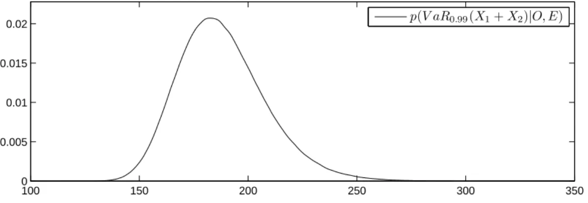
Suppose we are also interested in estimating the risk measure VaR0.99(X1+X2), i.e. the 99% Value-at-Risk of the aggregateX1+X2. The uncertainty in the parameters of the distri-bution of (X1,X2) naturally carries over to the uncertainty of a functional of (X1,X2), such as VaR0.99(X1+X2). We can estimate the posterior densityp(VaR0.99(X1+X2)|O,E) though nested Monte Carlo simulations. For each simulated parameter vector (θ,µ1,µ2,σ1,σ2), drawn from the posterior distribution, we draw a sample of size 10,000 from (X1,X2)|(θ,µ1,µ2,σ1,σ2). This sample allows to estimate VaR0.99(X1+X2), which provides one realization of the poste-rior distribution of VaR0.99(X1+X2)|O,E. Figure 3 shows the estimated densityp(VaR0.99(X1+ X2)|O,E).
100 150 200 250 300 350
0 0.005 0.01 0.015
0.02 p(V aR0.99(X1+X2)|O, E)
FIGURE 3. Posterior density of VaR0.99(X1+X2), estimated through nested Monte Carlo simulation.
Table 2 summarizes point estimates and associated uncertainties of the posterior distribu-tion of the parameters and VaR0.99(X1+X2). We also give the 90% credible interval, defined as the 5% and 95% quantile of the posterior distribution.
In practice, quantiles/VaRs are mostly estimated through parametric models (calibrated with maximum likelihood) or through techniques stemming from extreme value theory, such as the Peaks-over-Threshold method (POT), see McNeil et al. (2005). However, these tech-niques do not allow to incorporate expert opinion and confidence intervals derived from them may be of dubious quality for a small sample size. On the other hand, Bayesian infer-ence allows a natural representation of parameter uncertainty.
8. CONCLUSION
E[· |O,E] pvar(· |O,E) 90% credible interval
θ 0.335 0.056 [0.242, 0.428]
µ1 3.277 0.043 [3.207, 3.347]
µ2 2.957 0.068 [2.845, 3.069]
σ1 0.493 0.030 [0.447, 0.544]
σ2 0.792 0.048 [0.718, 0.877]
VaR0.99(X1+X2) 188.3 20.33 [158.3, 224.6]
TABLE 2. Statistics of the posterior distributions of θ, µ1, µ2, σ1, σ2 and
VaR0.99(X1+X2). We give posterior mean, standard deviation and the 90% credible interval.
separates the models and parameters for marginals and dependence structure. Through the Bayesian approach, uncertainties in the parameters can easily be accounted for. The same holds for functionals of (X1, . . . ,Xd), for instance for a risk measure applied toX1+ · · · +Xd. The model can also be used if not all of the three sources of information are available. For instance, the model allows to estimate model parameters and their uncertainty also if no observations (N=0) or no experts (K=0) are present.
Our method is most helpful in situations where observations are scarce, i.e. in cases where standard methods like maximum-likelihood usually exhibit severe parameter uncertainties. Asymptotic normality holds under mild smoothness and positivity assumptions on the prior and the conditional distribution of experts assessments. If the number of observations tends to infinity, the posterior will converge to the true value and point estimates are asymp-totically as efficient as maximum likelihood estimates.
We investigated the challenging process of turning expert opinion into quantitative in-formation. Certain principles deduced from psychological and statistical research must be adhered to in order to get reliable results. We propose procedures to assess the accuracy of the expert assessments through estimating their variance, which controls their weight in the final estimate. The Bayesian approach allows for natural interpretation of expert opinion.
ACKNOWLEDGEMENT
to significant improvements of the paper. As SCOR Fellow (P. Arbenz) and SCOR employee (D. Canestraro), the authors thank SCOR for financial support.
APPENDIXA. DEFINITION ANDPROPERTIES OF THEBETA DISTRIBUTION
A random variableZ ∈(0, 1) isBeta distributed, if its density is given by fZ(x)=xα−1(1− x)β−1/ B(α,β) for x∈(0, 1), whereα,β>0 and B(·,·) denotes the Beta function. Mean and variance are given byE[Z]=α/(α+β) and var(Z)=αβ/((α+β)2(α+β+1)). The parame-ters can be inferred from the moments throughα=E[Z]2(1−E[Z])/ var(Z)−E[Z] andβ= α(E[Z]−1−1). The beta distribution is unimodal ifα,β≥1 or, equivalently, if the variance satisfies var(Z)≤min©E[Z]2(1−E[Z])/(1+E[Z]), (1−E[Z])2E[Z]/(2−E[Z])ª.
The random variable a+(b−a)Z ∈[a,b] for some a <b is said to have a shifted Beta distributionwith endpointsa andb. Forθ close to the boundary ofΘ, a fixed conditional variance var(ϕk|θ)=σ2kcan be infeasible. For theseθ, we propose to reduce var(ϕk|θ) to the point whereϕk|θis unimodal.
REFERENCES
Bernardo, J. and Smith, A. (1994).Bayesian Theory. Wiley, Chichester.
Blum, P., Dias, A., and Embrechts, P. (2002). The art of dependence modelling: the latest advances in correlation analysis. In Lane, M., editor,Alternative Risk Strategies, pages 339–356. Risk Books, London.
Böcker, K., Crimmi, A., and Fink, H. (2010). Bayesian risk aggregation: Correlation uncertainty and expert judgement. In Böcker, K., editor,Rethinking Risk Measurement and Reporting Uncertainty. RiskBooks, London.
Bühlmann, H. and Gisler, A. (2005). A Course in Credibility Theory and its Applications. Springer, Berlin.
CEIOPS (2010). QIS5 Technical Specifications. Technical report, Committee of European Insurance and Occupational Pensions Supervisors.
Clemen, R., Fischer, G., and Winkler, R. (2000). Assessing dependence: Some experimental results. Management Science, 46(8):1100–1115.
Clemen, R. and Winkler, R. (1999). Combining probability distributions from experts in risk analysis. Risk Analysis, 19(2):187–203.
Cooke, R. (1991). Experts in Uncertainty: Opinion and Subjective Probability in Science. Oxford Uni-versity Press, New York.
Cooke, R. and Goossens, L. (2000). Procedures guide for structural expert judgement in accident consequence modelling.Radiation Protection Dosimetry, 90(3):303–309.
Cooke, R., Mendel, M., and Thijs, W. (1988). Calibration and information in expert resolution. Auto-matica, 24(1):87–94.
Daneshkhah, A. (2004). Uncertainty in probabilistic risk assessment: A review. Working paper, The University Of Sheffield. www.sheffield.ac.uk/content/1/c6/03/09/33/risk.pdf.
Donnelly, C. and Embrechts, P. (2010). The devil is in the tails: actuarial mathematics and the sub-prime mortgage crisis.ASTIN Bulletin, 40(1):1–33.
Eddy, D. (1982). Probabilistic reasoning in clinical medicine: Problems and opportunities. In Kah-neman, D., Slovic, P., and Tversky, A., editors,Judgment under uncertainty: Heuristics and biases, pages 249–267. Cambridge University Press, Cambridge.
Embrechts, P., McNeil, A., and Straumann, D. (2002). Correlation and dependence in risk manage-ment: Properties and pitfalls. In Dempster, M., editor,Risk Management: Value at Risk and Beyond, pages 176–223. Cambridge University Press, Cambridge.
Genest, C., Gendron, M., and Bourdeau-Brien, M. (2009). The advent of copulas in finance. The European Journal of Finance, 15(7–8):609–618.
Gokhale, D. and Press, S. (1982). Assessment of a prior distribution for the correlation coefficient in a bivariate normal distribution.Journal of the Royal Statistical Society, Series A, 145:237–249.
Hall, J. (2010).The Total Cost of Fire in the United States. National Fire Protection Association, Quincy, Massachusetts.
Haug, S., Klüppelberg, C., and Peng, L. (2011). Statistical models and methods for dependence in insurance data.Journal of the Korean Statistical Society, 40:125–139.
Hofert, M. (2010). Sampling Nested Archimedean Copulas with Applications to CDO Pricing. PhD thesis, University of Ulm.
Jouini, M. and Clemen, R. (1996). Copula models for aggregating expert opinions. Operations Re-search, 44(3):444–457.
Kahneman, D. and Tversky, A. (1973). On the psychology of prediction. Psychological review, 80(4):237–251.
Kahneman, D. and Tversky, A. (1982). On the study of statistical intuitions.Cognition, 11:123–141. Kallen, M. and Cooke, R. (2002). Expert aggregation with dependence. InProbabilistic Safety
ment and Management, pages 1287–1294. International Association for Probabilistic Safety Assess-ment and ManageAssess-ment.
Kynn, M. (2008). The “heuristics and biases” bias in expert elicitation. Journal of the Royal Statistical Society: Series A (Statistics in Society), 171(1):239–264.
Lambrigger, D., Shevchenko, P., and Wüthrich, M. (2007). The quantification of operational risk using internal data, relevant external data and expert opinions.Journal of Operational Risk, 2(3):3–27. McNeil, A., Frey, R., and Embrechts, P. (2005). Quantitative Risk Management: Concepts, Techniques,
Tools. Princeton University Press, Princeton.
Meyer, M. and Booker, J. (2001). Eliciting and Analyzing Expert Judgment: A Practical Guide. Society for Industrial and Applied Mathematics, Philadelphia.
Morgan, M. and Henrion, M. (1992).Uncertainty: A Guide to Dealing With Uncertainty in Quantitative Risk and Policy Analysis. Cambridge University Press, Cambridge.
Mosleh, A., Bier, V., and Apostolakis, G. (1988). A critique of current practice for the use of expert opinions in probabilistic risk assessment.Reliability Engineering and system safety, 20(1):63–85. Nelsen, R. (2006).An Introduction to Copulas. Springer, New York, 2nd edition.
O’Hagan, A., Buck, C., Daneshkhah, A., Eiser, J., Garthwaite, P., Jenkinson, D., Oakley, J., and Rakow, T. (2006)).Uncertain Judgements: Eliciting Experts’ Probabilities. Wiley, Chichester.
Ouchi, F. (2004). A literature review on the use of expert opinion in probabilistic risk analysis. Working Paper 3201, World Bank Policy Research.
Price, H. and Manson, A. (2002). Uninformative priors for Bayes’ theorem. Bayesian Inference and Maximum Entropy Methods in Science and Engineering, 617(1):379–391.
Robert, C. and Casella, G. (2005).Monte Carlo Statistical Methods. Springer, New York. Van der Vaart, A. (1998).Asymptotic Statistics. Cambridge University Press, Cambridge.
Winkler, R. (1968). The consensus of subjective probability distributions. Management Science, 15:B61–B75.
PHILIPP ARBENZ (corresponding author) RiskLab, Department of Mathematics Rämistrasse 101,
ETH Zurich
CH-8092 Zürich, Switzerland Tel: +41 44 6323428
Fax: +41 44 6321523
E-Mail: [email protected]